Credit ratings and government bonds: evidence before, during and after the european debt crisis

(1)

FUNDAÇÃO GETÚLIO VARGAS

ESCOLA DE ECONOMIA DE EMPRESAS DE SÃO PAULO

Miguel de Campos Pinto Coelho

CREDIT RATINGS AND GOVERNMENT BONDS

Evidence before, during and after the European debt crisis

(2)

FUNDAÇÃO GETÚLIO VARGAS

ESCOLA DE ECONOMIA DE EMPRESAS DE SÃO PAULO

Dissertação apresentada à Escola de Economia de Empresas de São Paulo da Fundação Getúlio Vargas, como requisito para obtenção do título de Mestre Profissional em Economia.

Campo do Conhecimento: International Master in Finance

Orientador Prof. Dr. João Mergulhão Prof. Dr. João Pedro Pereira

(3)

Pinto Coelho, Miguel.

Credit Ratings and Government Bonds: Evidence before, during and after the European debt crisis / Miguel Pinto Coelho. - 2016.

56 f.

Orientador: João de Mendonça Mergulhão, João Pedro Pereira Dissertação (MPFE) - Escola de Economia de São Paulo.

1. Dívida pública - Europa. 2. Dívida externa. 3. Déficit financeiro - Europa. 4. Taxas de juros. 5. Risco (Economia). I. Mergulhão, João de Mendonça. II. Pereira, João Pedro. III. Dissertação (MPFE) - Escola de Economia de São Paulo. IV. Título.

(4)

Dissertação apresentada à Escola de Economia de Empresas de São Paulo da Fundação Getúlio Vargas, como requisito para obtenção do título de Mestre Profissional em Economia.

Campo do Conhecimento: International Master in Finance

Data de Aprovação:

/ / .

Banca Examinadora:

Prof. Dr. João Mergulhão

Prof. Dr. João Pedro Pereira

(5)

Acknowledgements

I would like to express my gratitude to:

(6)

Resumo

Neste projeto, investigamos se as agências de rating e as taxas de juro de longo prazo da dívida soberana tiveram uma influência recíproca antes, durante e após a crise da dívida soberana Europeia. Esta análise é realizada, estimando a relação existente entre os ratings da dívida soberana ou taxas de juro e factores macroeconomicos e estruturais, através de uma diferente aplicação de metodologias utilizadas para este efeito. Os resultados obtidos demonstram que, no período da crise soberana, os ratings e as taxas de juros tiveram um mútuo impacto, sugerindo que as descidas dos ratings podem ter conduzido a profecias auto-realizáveis, levando países relativamente estáveis a um eventual incumprimento.

(7)

Abstract

This project investigates if there was any influence of credit rating agencies and long-term government bond yields on each other before, during and after Europe’s sovereign debt crisis. This is addressed by estimating the relationship and causality between sovereign debt ratings or bond yields and macroeconomic and structural variables following a dif-ferent procedure to explain ratings and bond yields. It is found evidence that, in distressed periods, ratings and yields do affect one another. This suggests that a rating downgrade might create a self-fulfilling prophecy, leading relatively stable countries to default.

(8)

List of Tables

1 Rating conversion . . . 42

2 Variables expected signal . . . 42

3 Explaining 10 year yield spreads with credit ratings . . . 43

4 Explaining 10 year yield spreads with and without Greece and dummies . 43 5 Explaining sovereign 10 year yield spreads for each period with dummies 44 6 Explaining ratings with 10 year yield spreads . . . 44

7 Explaining ratings with and without Greece and dummies . . . 45

8 Explaining ratings for each period with dummies . . . 46

9 Ordered probit model results for the determinants of credit ratings . . . . 47

A.1 Descriptive statistics for the entire sample period . . . 48

A.2 Descriptive statistics pre-crisis period . . . 48

A.3 Descriptive statistics crisis period . . . 48

A.4 Descriptive statistics post-crisis period . . . 49

A.5 Correlation matrix . . . 50

A.6 Correlation matrix pre-crisis . . . 50

A.7 Correlation matrix crisis . . . 51

A.8 Correlation matrix post-crisis . . . 51

A.9 Correlation matrix for the 10 year government bond spreads . . . 52

A.10 Correlation matrix for the 10 year government bond spreads pre-crisis . . 52

A.11 Correlation matrix for the 10 year government bond spreads crisis . . . . 53

A.12 Correlation matrix for the 10 year government bond spreads post-crisis . . 53

A.13 Correlation matrix for Moody’s Ratings . . . 54

A.14 Correlation matrix for Standard & Poor’s Ratings . . . 54

A.15 Correlation matrix for Fitch Ratings . . . 55

A.16 Correlation matrix for Moody’s Ratings pre-crisis . . . 55

A.17 Correlation matrix for Moody’s Ratings crisis . . . 56

(10)

List of Figures

(11)

Purpose of Project - General Overview

The global financial crisis of 2007 - 2010, which was once seen as an issue in the US sub-prime mortgage market and the bankruptcy of U.S. banks, evolved into a sovereign debt crisis in the Euro zone, with most European countries facing: (i) an abrupt increase

in the government bond yields and spreads against the German Bund; together with (ii)

successive downgrade of their credit ratings. In fact, until the end of 2009, Fitch Ratings, Inc. (“Fitch") would downgrade Greece’s credit rating from A- to BBB+ with a negative outlook, being the first time in almost 10 years that Greece had a rating below an A grade by any of the three major credit rating agencies.1 _{The Greece situation just intensified} the possibility of the Euro area collapse and increased the cost of financing of several countries, where the ones most affected were those with fragile fiscal situation. At the end of 2014, almost five years after the first bailout program during the European sovereign debt crisis, and after the austerity plans introduced by the countries most affected by it, Europe was facing a slow and long recovery. The majority of these countries saw their government bond yields and spreads fall to levels lower than the ones before the crisis was installed, some of them registered minimum values of both long- and short-term bond yields in their history. Nevertheless, credit ratings did not follow the exponential decrease in the yields, being some, still, considered as a speculative investment.

This thesis intends to explain the impact of the three most well know credit rating agencies (“CRA”), Fitch, Moody’s Investors Service, Inc. (“Moody’s”) and Standard & Poor’s Financial Services LLC (“Standard & Poor’s” or “S&P”), during the European sovereign debt crisis. In this context, it pretends to complement previous studies on the impact 1_{In “}_{Tough words and and hard budgets for eurozone}_{” (http://www.ft.com/cms/s/0/}

(12)

of sovereign rating changes and sovereign bond yield spreads on one another by using updated data (until December 31st_{, 2014) and through an analysis that will be performed} comparing the sovereign debt crisis period to the period before and after. In this sense, this paper pretends to assess how sovereign credit ratings influenced and were influenced by the bond yield spreads before, during and after the crisis.

The remainder of the thesis is organized as follows. In Chapter 2 it will be provided a review of related literature on the methodology behind sovereign debt ratings estimation and their role in the markets.

In Chapter 3, it will be given a description of the datasets used and reason of their appli-cation providing a methodological introduction.

Moreover, it will be described the empirical analysis and results of the impact of changes in the credit ratings issued by the CRA on the yield spread of sovereign bonds, vis-à-vis the German Bund, and vice-versa.

(13)

Literature Review

During the 1990s, the occurrence of several financial crises that affected the world fi-nancial markets led to an increase in popularity of the study of how CRA assessed the government’s creditworthiness and how ratings influenced the markets. More recently, the last financial crisis increased the concern about Greece’s, Portugal’s and Ireland’s capacity to pay their debts. This made investors turn to ratings as a measure of the cred-itworthiness of these countries and how the European Union was implementing measures to prevent a worldwide financial contagion.

In fact, the perception of sovereign risk of default published by Standard & Poor’s, Moody’s, and Fitch has a major role in the markets since it might ease the placement of sovereign debt in the primary markets. It also has a major impact for investors as the credit rating works as an “insurance” against the likelihood of default. Moreover, some institutional investors are obligated, either by law or their own statutes, to purchase and hold bonds with a certain minimum rating. Credit ratings are also used by regulators and market participants to establish the capital requirements and this could impact the portfo-lios since only highly rated assets are eligible as collateral to obtain credit. Under Basel II, countries, banks and corporations use the standardized approach to credit risk, which relies on credit ratings issued by external CRA to assess its own regulatory capital (i.e.,

the amount of capital required by the financial regulator).

A downgrade can, therefore, lead to a change in the demand for certain sovereign bonds hence increasing these countries yields and spreads against a benchmark (in Europe, spe-cially within the Euro area, it is usually used the German Bund as a benchmark).

(14)

two main categories. The first category concerns research that analyzes the determinants of sovereign credit ratings issued by CRA. Cantor and Packer (1996) analyzed a cross-section of 45 countries by applying OLS regressions to ratings and concluded that the rating is determined, mainly, by six economic factors - GDP per capita, GDP growth, inflation, external debt, level of economic development and default history - and that they are strongly correlated with market spreads. More recent studies by Bhatia (2002) and Afonso et al. (2007), the latter using a panel of 130 countries from 1970 to 2005, show similar conclusions with minor changes regarding the explanatory variables.

Other studies try to explain the impact of ratings on the yields and spreads of sovereign debt. Cantor and Packer (1996) realized that rating announcements directly affect the mar-ket although these often already anticipated the effects of this change (via the rise/decline of the spreads on the days before the announcement). Brooks et al. (2004) concluded, instead, that “only Sovereign ratings downgrades convey information to the market”.

The second category of research focused on the impact of CRA announcements during fi-nancial crisis. Ferri (1999) studied the impact during the East Asian fifi-nancial crisis, at the end of the 1990s, and concluded that rating agencies’ sovereign ratings may have aggra-vated it and that the CRA have failed to preventively warn the markets against the crisis. Mora (2006) then analyzed the “tremendous power to influence market expectations on a country” as pointed by Ferri (1999) and found out that ratings tend to be sticky (inertia of

sovereign ratings) and that they remain over-conservative after a crisis but that the impact should be analyzed more carefully.

(15)

Another topic covered by some of these studies and by other researchers is the spillover effect of one country rating downgrade and its impact in other countries’ ratings. Is-mailescu and Kazemi (2010), addressed this matter by evaluating the impact of credit rating changes, positive and negative, on the CDS spread of both the event country and other emerging economies. They concluded that there is evidence of immediate reaction of CDS markets to credit rating events.

Arghyrou and Kontonikas (2011) and De Santis (2012) applied the same rationale for the European Monetary Union (“EMU’) for the period up to the European sovereign debt cri-sis (roughly from 1999 to 2011, depending on the research) reaching a similar conclusion. They found that the early stage of the crisis was driven by the Greek debt crisis and that during the rest of the crisis period there is evidence for contagious from Greece, Portugal, Ireland and, on a lower scale, Spain and Italy (commonly referred as “PIGS” or “PIIGS”). This project contributes to the existent literature by explaining government bond yield spreads vis-à-vis the German Bund and sovereign credit ratings with a larger time period, covering the pre-European crisis, the crisis itself and post-crisis and using up to date data. This allows to capture how ratings and yields affect one another in different periods of a crisis and if there is, effectively, an impact.

Firstly, we will use in this study the linear regression approach following Cantor and Packer (1996) or Afonso et al. (2007) rationale and applying to panel data, regressions models for the ratings and yields.

Secondly, it will be used ordered models following Afonso et al. (2007) or Mora (2006) as ratings are a discrete variable and have different categories. The fact that the model used implies that the difference between two categories is the same for any two categories will not be addressed in this study.

(16)

Discussion of the Topic

3.1 Data

As referred above, credit rating agencies are specialized in the assessment of the likeli-hood of default of sovereign and corporate issuers. Due to the expansion of the number of countries issuing securities, the globalization of the capital market and the implemen-tation of laws and regulations as the Basel II, these agencies became protagonists in the financial markets.

This work project intends to study how far the CRA influenced or were influenced by the yield spreads of the countries during the crisis and what was this relation before and after this period.

For that purpose, we analyze quarterly 10-year yields and spreads, vis-à-vis the German Bund, from 12 economies: Austria, Belgium, Finland, France, Germany, Greece, Ireland, Italy, Netherlands, Portugal, Spain and United Kingdom (U.K.)1_{. The choice of these} countries is based on their differences namely, the size of the countries and the level of distress of these countries during the European sovereign debt crisis (“ESDC”) making them the perfect fit for the analysis. The sample period runs from the first quarter of 2002 (introduction of the Euro) until the last quarter of 2014. It was not considered more updated data in order for the financial data not to be influenced by the quantitative easing ("QE") program launched in early 2015 by the European Central Bank ("ECB"). In this sense, it is used the value of the yields of the last available business day of each quarter. Moreover, it is used the ratings issued by Moody’s, Fitch and Standard & Poor’s for all

(17)

these countries as they held together, in 2014, a global market share of roughly 90 percent 2_{. Although the analysis is similar for each rating, CRA do not use the same credit rating} notation therefore they were translated, based on previous literature (as used by Afonso et al. (2007)), into a numerical scale raging from 22 to 1 respectively, AAA or Aaa to D. In addition, a positive or negative credit watch announcement can foresee a rating change in the same direction in a near future. Taking this, it will also be analyzed the credit watch announcements from each CRA which will be translated to the numerical scale referred above and it will be valued±0.5 depending on it being a positive or negative credit watch. Table 1 on page 37, depicts the numerical conversion of each rating scheme, which sub-sequently will be used for the empirical analysis.

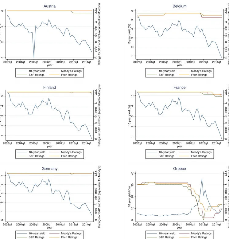
Figure 1 (page 35 and 36) show the evolution of the countries’ 10-year sovereign bond yield against the evolution of the ratings between the first quarter of 2002 and the last quarter of 2014. This figure shows a high correlation, during the crisis period, between rating changes and the increase on the yields, also revealing how ratings tend to have inertia (namely before and after this period).

Furthermore, the empirical analysis uses macroeconomic data as evidenced in the litera-ture (from Cantor and Packer (1996) to Afonso et al. (2007)):

• GDP Growth - In theory, higher GDP growth increases the capacity for

govern-ments to repay their debt and thus it is expected a negative impact on the yields and positive on ratings. Quarterly data on real GDP growth is from Eurostat.

• GDP per capita- A larger income per capita, measured in thousand euro per capita,

is anticipated in more developed (i.e., stable, strong) countries and it is expected to

have a negative impact on yields and a positive one on ratings. Quarterly data on GDP per capita is from Eurostat.

• Government surplus (i.e., surplus or deficit)- A higher deficit signals that the

(18)

ernment may not be able to repay its liabilities or that it will tax its population to cover its expenses. It is expected a negative effect on yields and positive on ratings. Quarterly data on government surplus as percentage of GDP is from Eurostat. • Inflation- Inflation rate may point for structural stability since stronger economies

have lower, but still positive, inflation in the medium term. A negative influence is expected for this on the rating and a positive for the yields. Quarterly data on inflation rate is from OECD.

• Unemployment - Distress periods usually lead to high unemployment rates and,

consequently, an increase in the social and economical burden of fiscal policy and social benefits. A positive impact on the yields and negative on ratings is expected. Quarterly unemployment rate is from Eurostat.

• Government debt - A higher government debt represents a higher risk of default

and thus it is expected to have a positive effect on the yields and a negative one on ratings. Quarterly data on government debt as percentage of GDP is from Eurostat. • Current account balance- A higher current account balance (external balance)

sig-nals that the government and/or companies rely heavily on domestic funds and, therefore, the economy tendency to over-consume “in house”. It is expected a pos-itive impact on ratings and negative on yields. Quarterly data measured as billions of euro is from Eurostat.

(19)

Moreover, the average of 4.20% for 10-year government bond yield and 1.15% for the 10-year government bond yield spread are also considerably low taking the crisis (again, the use of low-yield countries reduces considerably this value).

Such values could be more accurately analyzed if we split the all sample size in three periods: (i) before the crisis (from the first quarter of 2002 until the second quarter of

2008); (ii) crisis (from the third quarter of 2008 until the forth quarter of 2012); and (iii)

post-crisis (from the first quarter of 2013 until the last quarter of 2014). These sub-periods will be used throughout the text for further analysis.

Tables A.2, A.3 and A.4 of Appendix A show the descriptive statistics for each of the periods respectively, pre-, during and post-crisis.

From these it is perceived the gradual decline of the average ratings over time reflecting the situation lived in Europe. In what regards the average 10-year yields and spreads, it is possible to see a spike during the crisis and a decrease afterwards and, in the case of the yield, to levels below the ones before the crisis.

Notwithstanding the decrease of bond yields to minimum values from the first to the last period, the yield spreads did not follow this tendency, reflecting the change on the perception of the countries’ credit risk from one period to the other. In fact, whereas in the pre-crisis period investors assumed a similar risk for all countries, in the post-crisis one, it becomes evident to investors the difference in the credit risk associated with less fiscally stable and more fiscally stable countries.

More interesting than only considering the average yield, is to check the standard de-viation, as a simple measure for markets volatility (i.e., risk) over time. The standard

(20)

1,143% for the 1-year bond) before it was withdrawn of the market (a further analysis of the volatility will not be pursued during the current study).

3.2 Methodology

On a first section, the study of the relationship between ratings and yield spreads will partly follow the methodology used by Afonso et al. (2007).

The linear panel model used to estimate the yield spreadYi,t (vis-à-vis the German Bund)

of a countryi(i= 1, . . . , N), at timet(t= 1, . . . , T), is described as follow:

Yi,t =↵+ RRi,t+ Xi,t+ci+✏i,t (3.1)

whereRi,t is the rating of the country i at time t, Xi,t is a vector containing the

time-varying variables previously mentioned, the macroeconomic series, ci is an individual

effect and✏i,t represents an error term.

Moreover, it will be used a similar model to estimate the ratingRi,tof the same countryi (i= 1, . . . , N), at timet(t = 1, . . . , T):

Ri,t =↵+ YYi,t+ Xi,t+ci+✏i,t (3.2)

whereYi,t is the 10 year yield spread of countryiat timetandXi,t is a vector containing

the macroeconomic series,ci is an individual effect and✏i,trepresents the error term.

Generally speaking, to estimate this equation one can use pooled Ordinary Least Squares ("OLS"), fixed effect or random effect. According to Wooldridge (2001), “random ef-fect is synonymous with zero correlation between the observed explanatory variables and

the individual effect” whereas “the term fixed effect (. . .) means that one is allowing for arbitrary correlation between the unobserved effectciand the observed explanatory

(21)

and purely estimates↵, and as a multiple linear regression.

If the individual effect is uncorrelated with the regressors, E[ci|Xi,t, Yi,t] = 0, then the

random effect estimation is preferable. Nevertheless, if this condition is not verified, both pooled OLS and random effect provide inconsistent estimates and hence one should use fixed effects. In our study, it is expected for the individual effect to be correlated with the regressors hence it will be used the fixed effects estimation.

Moreover, heteroskedasticity is present in the model if the variance of the error terms changes. Consequently, we correct for heteroskedasticity by using robust standard errors. The main purpose of the first section is to obtain robust indicators on how CRA can influence or are influenced by the yield spreads of the countries. For that we will use macroeconomic factors and credit ratings/spreads as a proxy for risk as it is commonly done in comparable studies. On the contrary, with the division of the analysis in subperi-ods it is expected to contribute to the literature by studying how this relation has changed over different economic periods.

On a second section, and taking the limited (i.e., discrete) structure of the credit ratings,

the ordered framework will be used. For this purpose, it will be computed a ordered probit model as follow:

R∗i,t = 0

Xi,t+✏i,t (3.3)

whereXi,t is the vector of variables that explains the variation in ratings and✏i,t is the

disturbance term that are assumed to be normally distributed.

Due to the limited structure of the credit ratings, several cut-off points will be computed to establish the boundaries for each rating level. R∗

i,t, which represents a continuous

(22)

3.3 Empirical Analysis

3.3.1 Correlation

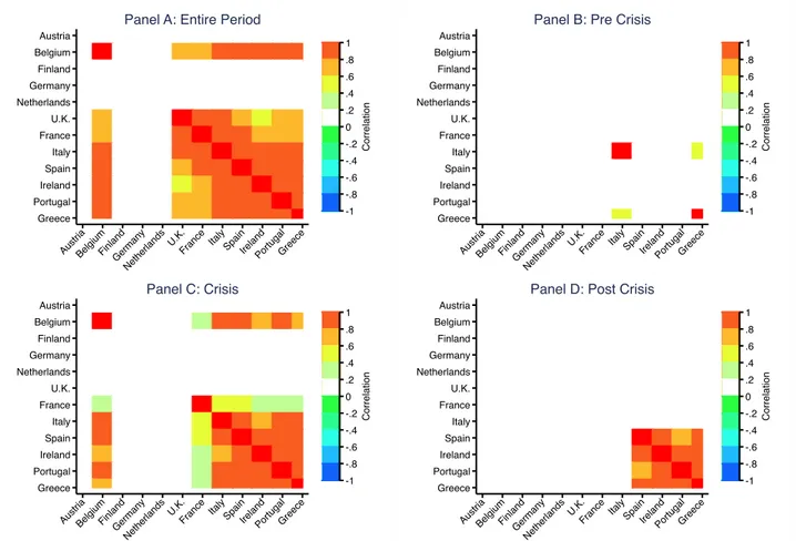
Before proceeding to the analysis of the estimation models, it is important to analyze the correlation between the variables as well as the correlations between the CRA and the 10-year yield spread, separately, within countries. Table A.5 through A.8 in Appendix A show the correlation matrices of the parameters for the four periods above mentioned (all sample period, pre-crisis, crisis and post-crisis).

From the first table we can realize the negative correlation between the CRA and the 10-year yield spreads confirming the intuition that an increase in the rating would result in a decrease in the spreads, and vice-versa. In addition, the majority of the macroeconomic variables’ correlation with the 10-year yield spread meet the expected relation beforehand stated (with the exception of inflation).

Again, the values in this table do no fully explain the correlation over time between these variables. The level of correlation between the CRA and the 10-year yields spread changed as the crisis materialized. In fact, during this distress period the correlation between these two variables changed, from around4% to −88%. But not only did the

correlation between these two variables changed but so did the correlation between the remaining variables and the spread with 8 out of 10 correlations with its sign changing from one period to the next, being the exceptions for this result the inflation and gov-ernment surplus. Moreover, for all the variables, the absolute value of the correlation increased from the period before the crisis to the crisis one.

(23)

de-crease of the spreads in recent years. Austria Belgium Finland Germany Netherlands U.K. France Italy Spain Ireland Portugal Greece Aust ria Belg ium

Finland_Germa ny

Net herla

nds U.K. France ItalySp

ain Irela nd Portu gal Gre ece -1 -.8 -.6 -.4 -.2 0 .2 .4 .6 .8 1 C o rre la ti o n

Panel A: Entire Period

Austria Belgium Finland Germany Netherlands U.K. France Italy Spain Ireland Portugal Greece Aust ria Belg ium

Finland_Germa ny

Net herla

Panel B: Pre Crisis

Austria Belgium Finland Germany Netherlands U.K. France Italy Spain Ireland Portugal Greece Aust ria Belg ium Finland Germa ny Net herla

Panel C: Crisis

Panel D: Post Crisis

Figure 3.1: Correlation heat maps of 10-year bond yields before, during and after crisis

(24)

With the creation of the European Monetary Union (“EMU”) the countries that adopted the Euro saw their yields decrease reflecting the elimination of exchange rate risk, the harmonization of the fiscal policies and a more integrated debt market (Figure 3.2).

4 6 8 10 12 1 0 ye a r yi e ld (% )

1/1/1990 1/1/1992 1/1/1994 1/1/1996 1/1/1998 1/1/2000 1/1/2002 Date

Austria Belgium Finland

France Germany Greece

Ireland Italy Netherlands

Portugal Spain U.K.

Source of data: Bloomberg

Government 10 year bond yields before Euro

Figure 3.2: Government 10 year bond yields before Euro introduction

Likewise, the European Central Bank’s practice of valuing all euro area countries’ bonds on the same terms as collateral for central bank credit to banks led investors to assume a similar risk for all countries. Such convergence is observed in Panel B of Figure 3.1 (Table A.10 of Appendix A) where there is a high positive correlation

between all the countries that were in the process of entering the EMU in contrast with the correlation between these countries and the U.K.

Greek Bailout

Irish Bailout Portuguese Bailout

Greek Bailout II

0 10 20 30 40 1 0 ye a r yi e ld (% )

1/1/2002 1/1/2004 1/1/2006 1/1/2008 1/1/2010 1/1/2012 1/1/2014

Date

Austria Belgium Finland

France Germany Greece

Ireland Italy Netherlands

Portugal Spain U.K.

Source of data: Bloomberg

Government 10 year bond yields after Euro

Figure 3.3: Government 10 year bond yields after Euro introduction

The implosion of the crisis, the quickly de-terioration of macroeconomic fundamen-tals for some countries and the rise of gov-ernment debt to unbearable levels accen-tuated fiscal stimulus measures on some economies leading to increasing costs of financing in the markets and, ultimately, to divergences of the yields (Figure 3.3).

This reaction is clear in the negative correlation between the countries that were affected the most by the crisis and those with stronger fiscal fundamentals revealing a shift of the investors demand for countries’ debt from the first group to the latter (Figure 3.1, Panel C and Table A.11 of Appendix A).

(25)

successful financial assistance programs of Ireland and Portugal relieved the markets and led to an overall decrease of the yields in the EMU and, consequently, to a positive cor-relation between the countries’ yield spreads - Panel D of Figure 3.1 and Table A.12 of Appendix A.

Furthermore, Table A.13 through A.15 show the correlation matrices for each of the CRA. In this regard, it is only analyzed the correlation between the countries with more signifi-cant changes in ratings (countries that did not face a rating change over the period under analysis do not have a correlation defined hence are depicted in the tables with a "."). During the crisis period, Moody’s decreased “Portugal’s long-term government bond rat-ings to Ba2 from Baa1 and assigned a negative outlook”3, not only on the basis of weak

macroeconomic fundamentals but also as a reaction of the situation lived in Greece. As so, a high correlation level would be expected between these two countries. Furthermore, it is equally expected a high correlation between these two countries and Ireland, the third intervened country, as the situation in Greece also had an implication on Ireland’s rating downgrades4_.

In addition, one could also expect: (i) a contagion of the Portuguese situation to Spain,

as this country is a major holder of Portuguese debt5_{and (}_ii_{) a higher correlation between} France, Italy and Spain and the remaining major economies than between these and the intervened countries since a distress situation in France, Italy or Spain would have a higher impact on European economies than the impact of a less economically powerful country as Portugal, Greece or even Ireland.

All these relations can be seen the tables. It is shown the high correlation between Por-tugal, Ireland and Greece signaling a contagion effect between these economies. Spain 3_{In “}_{Moody’s downgrades Portugal to Ba2 with a negative outlook from Baa1}_{” (https://www.}

moodys.com/research/Moodys-downgradesPortugal-to-Ba2-with-a-negative-outlook-from? lang=en&cy=global&docid=PR_222043)

4_{In “}_{Moody’s downgrades Ireland to Ba1; outlook remains negative}_{” (https://www.moodys.}

com/research/Moodys-downgrades-Ireland-to-Ba1-outlook-remains-negative--PR_ 222257)

5_{In “}_{Eurozone debt web:} _{Who owes what to whom?} _{(http://www.bbc.com/news/}

(26)

is highly affected by rating changes in Portugal with the CRA clearly relating its level of risk with the amount of risky assets (Portuguese bonds) that it held.

Moreover, Spain, which had to intervene in the banking system with Madrid lending over

e40 billion to Spanish banks and nationalizing of Bankia6 (the country’s fourth-largest

bank by Tier 1 capital in 20147_{) saw their yield spreads vis-à-vis the Germand Bund} increase to levels around 6% in this period and several downgrades in the banking system and the country’s ratings.

France, on the contrary, is the country with less impact in its ratings from the situation lived in other economies. Yet, a change in the rating of France is more related with changes in the ratings of Spain and Italy, as these are the major economies affected by the sovereign debt crisis, and that are highly correlated between them.

Table A.16 through A.18 are for Moody’s ratings correlation before, during and after crisis. This is also depicted in Figure 3.4 below, from Panel B through D, respectively. In the pre-crisis period, there are no material changes in ratings with most of the coun-tries maintaining its ratings for the entire period. In the crisis period, it is possible to verify a high correlation between fiscally "weaker" countries and the absence of correla-tion between these countries and fiscally stronger ones. France has a low correlacorrela-tion with Portugal, Ireland or Greece and stronger one with other big economies as Spain or Italy. On the other hand, these last two countries have a high positive correlation between them and with the remaining PIIGS with the increase in stability of Italy leading to an absence of correlation with Spain, Portugal, Ireland or Greece after this period.

Spain, Portugal, Ireland and Greece, on the contrary, have, as expected, a high positive correlation both during and after the crisis with a persistence of high correlation between Ireland and Portugal from one period to another and a decrease of correlation between 6_In _“_Spain’s _Bankia-Led _Bailout _Won’t _Spell _End _of _Bank

Trou-bles” (http://www.bloomberg.com/news/articles/2013-02-27/

spain-s-bankia-led-bailout-won-t-spell-end-of-troubles-for-banks)

7_In _“_The _top _five _Spanish _banks_” _{(http://www.thebanker.com/Banker-Data/}

(27)

these countries and Greece. This result could be partially explained by the “end” of the financial assistance program in Ireland in December 2013 followed, only a few months later, by Portugal, leading to a regain of the market’s confidence and hence an increase in the ratings of these countries.

nds U.K.

France ItalySp

Panel A: Entire Period

nds U.K.

France ItalySp

Panel B: Pre Crisis

Finland_Germa ny

Net herla

Panel C: Crisis

Finland_Germa ny

Net herla

Panel D: Post Crisis

Figure 3.4: Correlation heat maps of Moodys’ ratings before, during and after crisis

3.3.2 Models interpretation

Rating on yield

(28)

for that purpose, the formerly mentioned fixed effects. The models are divided by rating: (i) Moody’s for 1 and 2; (ii) S&P for 3 and 4; and (iii) Fitch for 5 and 6. Moreover,

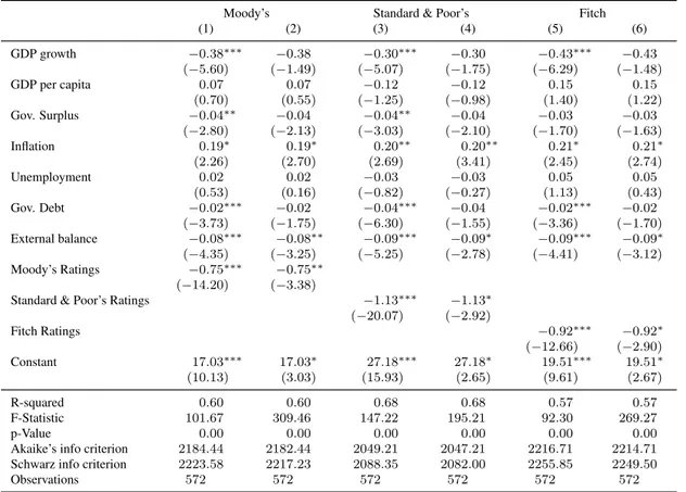
odd number models represent the simple fixed effects model while even number models represent the simple fixed effect model but with heteroskedasticity-robust coefficients. The most influential factors for the yield spreads of the countries are the ratings, inflation and external balance, which are robustly statistically significant at least at a 10% signif-icance level over the three CRA. Credit ratings and inflation have the expected impact on yield spreads [an upgrade (increase) of the rating (inflation) decreases (increases) the spread] but, on the other hand, government debt has a contradictory impact as an increase of the indebtedness level decreases the yield spread. The minimum amount of govern-ment debt around 24% of gross domestic product (“GDP”) and, specially a mean of 77% of GDP over the whole period, might undervalue the impact of debt in the yields.

Another explanation is, again, the lag between financial and macroeconomic fundamen-tals adjustments. After the crisis period (2013 onwards), and due to delivery of the assis-tance programs tranches to Greece, Portugal and Ireland, these countries saw their debt increase whereas the markets perception of risk eased and, consequently, the correspon-dent government yield spreads decreased, vis-à-vis the German Bund, in the secondary market.

The models obtained by this process point for similar results across the three CRA. As so, it will be used Moody’s as a proxy for the impact of rating agencies in the yields spreads, and vice-versa.

(29)

coun-tries under analysis, even against Ireland and Portugal.

In this sense, and now that it has been covered the base model for the analysis of the yield spreads for comparison, the first step will be to reestimate the model, again as panel data, but without considering Greece. The robust results are in the first two columns (first with Greece and second without) of Table 4 (page 38).

The not inclusion of Greece in the estimation provides much clearer analysis of the eco-nomic situation lived in Europe. The first difference worth to emphasize is the decrease of the constant (base level of the 10-year yield spread) by 8% indicating the impact of Greece’s high level of 10-year yield spread over the whole period (Greece, within the sample, reached a maximum value of 35% and had, more often than not, higher yields than its counterpart countries).

Furthermore, not accounting for the default of a country in the estimation allows for the CRA coefficient to decrease by almost one half, yet staying significant indicating that CRA do have a role in the yield level of a country.

The two last significant changes are: (i) government surplus is now robustly significant at

a 10% significance level; and (ii) inflation, though its signal remains the same, becomes

statistically insignificant.

To account for the specificities in the data and the robustness of the results we included several variables such as a dummy for the period with financial assistance (which de-pended on the country) or variables to account for specific rules of the EMU as the deficit above 3% or the debt level above 60%. These variables turned out statistically insignifi-cant in the sample used.

Instead of a debt level above 60%, it was used a benchmark of 90% of GDP as a variable to distinguish between countries. The robust results, which do not include Greece again, are depicted in the third column of Table 4 [model (3)]. In this context, "Gov. Debt≥90" is

(30)

change of the government debt of a country which has a debt level as a percentage of GDP above 90%. Comparing model (2) and (3), Gov. Debt≥90 is not statistically significant

and the coefficient has a neutral value indicating that the increase of government debt level by 1% is the same for countries with a high or low government debt.

Some literature also uses dummies for the crisis period, Greece or the PIGS to estimate the impact of CRA on yields (see Gärtner et al. (2011) for comparative analysis). In light of this procedure it was computed series of models using a specific dummy the crisis period and an interaction term between Greece and the rating. The results are shown in the last two columns of Table 4 and include the interaction term for a debt level higher than 90% of GDP previously used.

Both these models give a similar result the one from the panel data analysis above. Moody’s, government surplus and inflation are statistically significant and with identi-cal signs but now external balance is no longer significant.

Furthermore, the interaction term between Moodys and Greece turned out to be statisti-cally significant indicating that a downgrade of the Greek rating by one notch by Moody’s has an impact on Greece’s yield spread approximately 0.4% higher than a similar decrease on other countries’ rating. The dummy for the crisis period is also statistically significant (at a 10% level) and indicates that in this period, the yield spread of the countries vis-à-vis the German Bund is,ceteris paribus, 1.46% higher than in the remaining periods.

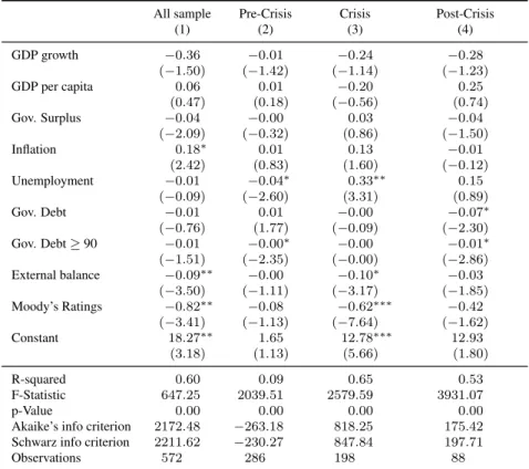
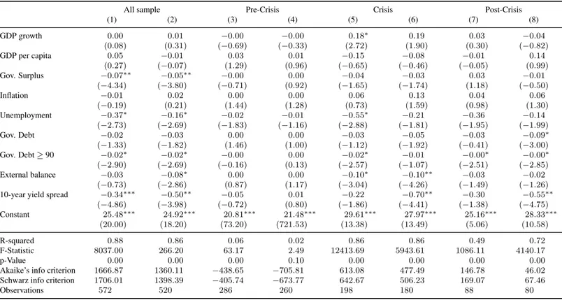
From all the previous models it is possible to see that the rating variable is always sta-tistically significant, but how does the rating impact changes over time? Table 5 on page 39 depicts four robust models, where model 1, 2 ,3 and 4 are, respectively, for all sample period, pre-crisis period, during crisis period and post-crisis period.

(31)

An increase in the credit ratings has, as expected, a statistically significant negative impact of the on yield spreads during the crisis -i.e., a downgrade of the rating leads to an increase

of the yield spreads. Additionally, the impact intensified during the crisis, from -0.08% to -0.62%. Nevertheless, a high amount of downgrades during the crisis, even for fiscally stable countries which did not face a spike in their yield spreads, could have reduced the expected impact of the ratings on the yields.

During this period, not only the majority of the countries faced a rating change (either of credit watch or effective rating change), but the rating changes themselves were larger than in other periods. Thus, yield spreads are explained by a change in the rating but, more importantly, by the magnitude of this change (for Greece, the magnitude of the change on the rating was of 16 leading to a change in the yield spread,ceteris paribus, of 9.92%).

In the post-crisis period, and although it is not statistically significant, the impact of rat-ings on yields eases to -0.41% indicating that a rating upgrade, in this period, had a lower impact on the yield spreads than a similar downgrade during the crisis period. Moreover, this results partly reflects the inertia of the ratings when considering the fact that yield spreads decreased sharply to minimum historical values while ratings felt slight upgrades. These results clearly indicate that the credit ratings do/did have an impact on the sovereign yield spreads of the countries and that, due to the high amount of downgrades, ended up aggravating the crisis in Europe.

Yield on rating

(32)

capita, the lower will be the credit rating,ceteris paribus.

Inflation, which is statistically insignificant to help explaining all the three ratings, also has the opposite signal indicating that a higher inflation leads to better ratings. The low variability of this variable, both considering all sample period or within each subperiod, may lead to such result. Focusing on the yield spread, in what regards all the CRA, an increase of 2% of the yield spread would lead to a reduction of the rating of, at least, 0.5 which is equivalent to a negative credit watch.

Again, for the remaining of the analysis, and considering the similarity of the results, it will be only used the Moody’s rating as a proxy for the ratings.

Previously, the model with or without Greece provided a different insight about the yields estimation. A similar procedure is done for the ratings and the results are depicted in the first two columns Table 7 (model 1 and 2 with and without Greece, respectively) on page 40. Now, the non-inclusion of Greece slightly changes the previous results with an increase of 2% on the yield spread leading to a decrease by 1 notch of the rating. The inclusion of interaction term for debt higher than 90% of GDP, as presented in the third model of Table 7, reduces the impact of a change of yield spreads on ratings and it is, now, statistically significant. In this case, an increase in government debt of a country with a debt higher than 90% of GDP has, ceteris paribus, higher decrease of the rating than a

similar change in a country with a more stable fiscal situation.

The last two columns present a model including a dummy for the crisis period and the interaction term for the debt as above mentioned, with (4) and without Greece (5). The results are fairly similar to the ones previously obtained with the dummy for the crisis period being statistically significant in both models and indicating that, during this period, the rating is higher, ceteris paribus. This unexpected value is offset by the increase,

(33)

verified in this is around 33% considering Greece, a much larger value than 1.14% and 11.15% for the other periods. In this sense, the value of the dummy is completely offset by a positive change on the yields of 2% which, during this period, was verified for the majority of the countries studied. The countries for which this dummy has a clear impact are the ones with a more stable fiscal situation as Austria, Finland or Netherlands.

Table 8 (page 41) decomposes the rating estimation for the 4 periods under analysis (all sample, pre-, during- and post-crisis) with and without Greece. The first different result is that, before the crisis, none of the variables had a statistically significant impact on the rating contradicting the results existing in the literature. Nevertheless, this period was a relatively stable one, a period which followed an effort by the countries to fulfill the euro convergence criteria introduced by the Maastricht Treaty: (i) price stability (via HCPI);

(ii) sound public finances (government deficit not more than 3% of GDP); (iii)

sustain-able public finances (government deficit not more than 60% of GDP); (iv) durability of

convergence (via long-term interest rates); and (v) exchange rate stability, which had to

be met in order for the countries to be eligible to enter the EMU.

(34)

during this period, this results provides information about why ratings of “weaker” coun-tries were downgrade by such a large amount (a 15% increase on the yield spread, as the one in Greece, would lead to downgrade of three notches).

The exclusion of Greece from the sample makes the yield spread statistically significant though GDP growth and unemployment are no longer significant. Now, the 10% increase in the spread of Portugal during the crisis period would traduce into a downgrade of seven notches of Moody’s rating.

The post-crisis period provides a different insight and, with the inclusion of Greece, no variables are statistically significant indicating, again, the existence of ratings inertia after a crisis period as mentioned by Mora (2006). The exclusion of Greece from the sample makes government debt and the yield spread statistically significant variables and a 3% decrease in the Portuguese spread would lead to a an upgrade of the rating by one notch and a positive credit watch (a numerical value of 1.5),ceteris paribus. During this period,

Portugal did face indeed an upgrade by two notches of the Moody’s rating yet, high levels of government debt and lower decreases of the spread than the increase verified during the crisis could help explain the inertia of the ratings in this last period.

So far, it has been shown that, during the crisis, ratings had an impact on spreads (and spreads on ratings if Greece is excluded from the sample) helping a self-fulfilling prophecy on the countries instability at a structural and markets level. For the remaining periods, and if Greece is included, the two variables revealed not to be statistically significant. Moreover, before the crisis, none of the variables here studied had an impact either on the ratings or on yield spreads.

As mentioned before, a different approach to analyze what determines the ratings is to use an ordered probit model as in equation 3.3. Table 9 on page 42 depicts the ordered probit model to determine the Moody’s rating for all the sample period, the pre-crisis period, the crisis period and the post-crisis period.

(35)

inclusion of Greece, in the pre-crisis period, GDP per capita, unemployment and govern-ment debt are statistically significant in all four periods. External balance is statistically significant in every period with the exception of the post-crisis one and GDP growth and 10-year yield spreads are only statistically significant in this last period.

In the pre-crisis period, an increase in the GDP per capita, government debt or external balance would result in the expected change in the rating. Unemployment, on the con-trary, has an unexpected impact, with an increase in the unemployment level of a country, leading to an upgrade of the rating.

With the exception of Greece, GDP per capita has a positive trend throughout time in all the countries yet the stagnation on the last two periods for some countries and the decrease of this variable in Greece, Italy or Portugal to levels similar to late 2003/early 2004 together with the downgrade during the crisis and then the slight improvement of the ratings in the post-crisis period might explain why this variable has slight positive impact during the crisis and negative in post-crisis model, respectively.

Furthermore, the impact of the yield spread more than doubles from the crisis period to the post-crisis one which could be due, as previously mentioned, to a larger change of the yield spread relative to the change in the ratings after the crisis than during it reflecting the fact that, after the crisis, yield spreads dropped to levels closer to the ones before the crisis but the ratings were not upgraded to the levels before the crisis or similar.

(36)

Conclusion

The objective of this study was to assess the extent of influence of credit rating announce-ments on sovereign bond yield and the influence of a change on the yields to credit rating focusing on the European market.

For this purpose it was used 10-year sovereign bond yield spreads, vis-à-vis the German Bund, and macroeconomic data from 12 European economies for a period between 2002 and 2014 and divided into three major periods: (i) the period before the crisis (from the

first quarter of 2002 until the second quarter of 2008); (ii) the financial crisis and the

sovereign debt crisis period (third quarter of 2008 until the last quarter of 2012); and (iii)

the period after the crisis (first quarter of 2013 until the last quarter of 2014).

We estimated the impact of credit rating announcements (i.e., changes in rating grades

and credit watch), made by Moody’s (as a benchmark) throughout these periods, focusing the study on two models: (i) panel data regression models including dummy variables

for different situations; and (ii) ordered models. The main contribution is providing an

updated study on the impact of credit rating agencies and spreads on one another not limiting the study to selected periods (such as the crisis) and extending previous analysis to a period after a crisis.

(37)

studied by the majority of the references above.

Regarding the analysis per sub-period, the results vary for the different periods. For the first methodology (i.e., panel regressions), confirm that ratings had an impact on the yield

spreads during the crisis though, both in the pre- and post-crisis period, this impact is not statistically significant. Moreover, the inclusion of different dummy variables and interaction terms turned out to be statistically insignificant and inconclusive regarding its impact on yield spreads including the interaction term for government debt higher than 90% of GDP. Other variables as the interaction term of Moody’s and Greece and a dummy for the crisis period turned out to be statistically significant indicating that yield spreads tend to be higher during a crisis and that a change in Moody’s rating had a higher impact on Greece than a similar one for the remaining countries.

The study of the impact of the yield on the credit ratings provided similar results in both methodologies when considering the 12 years under analysis. Both models indicate that yield spreads had an impact on the ratings. Moreover, the majority of the variables had an impact on the ratings which goes according to what one might expect considering that credit ratings provide information about present and future state of the economy.

(38)

In light of the above, it is possible to assume that, during the crisis, ratings announcements (either credit watch or rating changes) and the information that it provides to the markets had a direct impact on sovereign yields. However, during the remaining periods analyzed, the results do not show that, these same announcements provide enough information to significantly change yields on the secondary markets. The results with Greece, on the contrary, do not provide clear information about the effect of the increase of spreads during the crisis and the decrease after, on ratings.

The possible extensions of this study are diverse. Given the methodology and the results, it is suggested to apply it to often forgotten bond markets of emerging countries. Moreover, it would be interesting to apply these model to more countries and for a broader period or even different crisis (as the Asian crisis) and compare for the same different subperiods (before, during and after a crisis).

(39)

Bibliography

Afonso, A., Gomes, P., and Rother, P. (2007). What “hides” behind sovereign debt rat-ings? Working Paper Series 0711, European Central Bank.

Arghyrou, M. G. and Kontonikas, A. (2011). The EMU sovereign-debt crisis: funda-mentals, expectations and contagion. SIRE Focus Paper 2011-01, Scottish Institute for Research in Economics (SIRE).

Bhatia, A. V. (2002). Sovereign Credit Ratings Methodology; An Evaluation. IMF Work-ing Paper 02/170, International Monetary Fund.

Brooks, R., Faff, R. W., Hillier, D., and Hillier, J. (2004). The national market impact of sovereign rating changes. Journal of Banking & Finance, 28(1):233–250.

Cantor, R. and Packer, F. (1996). Determinants and impact of sovereign credit ratings.

Economic Policy Review, 2(2):37–53.

De Santis, R. A. (2012). The Euro area sovereign debt crisis: safe haven, credit rating agencies and the spread of the fever from Greece, Ireland and Portugal. Working Paper Series 1419, European Central Bank.

Ferri, G. (1999). The procyclical role of rating agencies : evidence from the East Asian crisis.

Gärtner, M., Griesbach, B., and Jung, F. (2011). PIGS or Lambs? The European Sovereign Debt Crisis and the Role of Rating Agencies. Economics Working Paper Series 1106, University of St. Gallen, School of Economics and Political Science. Ismailescu, I. and Kazemi, H. (2010). The reaction of emerging market credit default

swap spreads to sovereign credit rating changes. Journal of Banking & Finance,

34(12):2861–2873.

Mora, N. (2006). Sovereign credit ratings: Guilty beyond reasonable doubt? Journal of Banking & Finance, 30(7):2041–2062.

Wooldridge, J. M. (2001). Econometric Analysis of Cross Section and Panel Data. The

(40)

Figures

AAA A BBB BB B CCC D

Ratings for S&P and Fitch (equivalent for Moody’s)

0

2

4

6

10 year yield (%)

2002q1 2004q1 2006q1 2008q1 2010q1 2012q1 2014q1 year

10−year yield Moody’s Ratings S&P Ratings Fitch Ratings

Austria AAA A BBB BB B CCC D

1 2 3 4 5 6

10 year yield (%)

2002q1 2004q1 2006q1 2008q1 2010q1 2012q1 2014q1

year

10−year yield Moody’s Ratings

S&P Ratings Fitch Ratings

Belgium AAA A BBB BB B CCC D

1

2

3

4

5

10 year yield (%)

2002q1 2004q1 2006q1 2008q1 2010q1 2012q1 2014q1 year

Finland AAA A BBB BB B CCC D

1

2

3

4

5

10 year yield (%)

2002q1 2004q1 2006q1 2008q1 2010q1 2012q1 2014q1 year

France AAA A BBB BB B CCC D

0 1 2 3 4 5

10 year yield (%)

2002q1 2004q1 2006q1 2008q1 2010q1 2012q1 2014q1 year

Germany AAA A BBB BB B CCC D

0

10

20

30

40

10 year yield (%)

2002q1 2004q1 2006q1 2008q1 2010q1 2012q1 2014q1

year

Greece

(41)

AAA A BBB BB B CCC D

2 4 6 8 10 12

10 year yield (%)

2002q1 2004q1 2006q1 2008q1 2010q1 2012q1 2014q1

year

Ireland AAA A BBB BB B CCC D

2 3 4 5 6 7

10 year yield (%)

2002q1 2004q1 2006q1 2008q1 2010q1 2012q1 2014q1 year

Italy AAA A BBB BB B CCC D

1

2

3

4

5

10 year yield (%)

2002q1 2004q1 2006q1 2008q1 2010q1 2012q1 2014q1 year

Netherlands AAA A BBB BB B CCC D

0

5

10

15

10 year yield (%)

2002q1 2004q1 2006q1 2008q1 2010q1 2012q1 2014q1 year

Portugal AAA A BBB BB B CCC D

2

3

4

5

6

10 year yield (%)

2002q1 2004q1 2006q1 2008q1 2010q1 2012q1 2014q1 year

Spain AAA A BBB BB B CCC D

2

3

4

5

6

10 year yield (%)

2002q1 2004q1 2006q1 2008q1 2010q1 2012q1 2014q1 year

U.K.

(42)

Tables

Table 1: Rating conversion

Credit Rating Moody’s S&P/Fitch Numerical Value

Investment Aaa AAA 22

grade Aa1 AA+ 21

Aa2 AA 20

Aa3 AA- 19

A1 A+ 18

A2 A 17

A3 A- 16

Baa1 BBB+ 15

Baa2 BBB 14

Baa3 BBB- 13

Speculative Ba1 BB+ 12

grade Ba2 BB 11

Ba3 BB- 10

B1 B+ 9

B2 B 8

B3 B- 7

Caa1 CCC+ 6

Caa2 CCC 5

Caa3 CCC- 4

Ca CC 3

C C 2

D 1

Credit watch

Positive 0.5

Negative −0.5

Table 2: Variables expected signal

Expected signal Dependent 10-year _Rating

variable yield spread

GDP growth - +

GDP per capita - +

Gov. Surplus - +

Inflation +

-Unemployment +

-Gov. Debt +

-External balance - + Moody’s Ratings

-S&P Ratings -Fitch Ratings

(43)

-Table 3: Explaining 10 year yield spreads with credit ratings

Moody’s Standard & Poor’s Fitch

(1) (2) (3) (4) (5) (6)

GDP growth −0.38⇤⇤⇤ ₋₀_.₃₈ ₋₀_.₃₀⇤⇤⇤ ₋₀_.₃₀ ₋₀_.₄₃⇤⇤⇤ ₋₀_.₄₃

(−5.60) (−1.49) (−5.07) (−1.75) (−6.29) (−1.48) GDP per capita 0.07 0.07 −0.12 −0.12 0.15 0.15

(0.70) (0.55) (−1.25) (−0.98) (1.40) (1.22) Gov. Surplus −0.04⇤⇤ ₋₀_.₀₄ ₋₀_.₀₄⇤⇤ ₋₀_.₀₄ ₋₀_.₀₃ ₋₀_.₀₃

(−2.80) (−2.13) (−3.03) (−2.10) (−1.70) (−1.63) Inflation 0.19⇤ ₀_.₁₉⇤ ₀_.₂₀⇤⇤ ₀_.₂₀⇤⇤ ₀_.₂₁⇤ ₀_.₂₁⇤

(2.26) (2.70) (2.69) (3.41) (2.45) (2.74) Unemployment 0.02 0.02 −0.03 −0.03 0.05 0.05

(0.53) (0.16) (−0.82) (−0.27) (1.13) (0.43) Gov. Debt −0.02⇤⇤⇤ ₋₀_.₀₂ ₋₀_.₀₄⇤⇤⇤ ₋₀_.₀₄ ₋₀_.₀₂⇤⇤⇤ ₋₀_.₀₂

(−3.73) (−1.75) (−6.30) (−1.55) (−3.36) (−1.70) External balance −0.08⇤⇤⇤ ₋₀_.₀₈⇤⇤ ₋₀_.₀₉⇤⇤⇤ ₋₀_.₀₉⇤ ₋₀_.₀₉⇤⇤⇤ ₋₀_.₀₉⇤

(−4.35) (−3.25) (−5.25) (−2.78) (−4.41) (−3.12) Moody’s Ratings −0.75⇤⇤⇤ ₋₀_.₇₅⇤⇤

(−14.20) (−3.38)

Standard & Poor’s Ratings −1.13⇤⇤⇤ ₋₁_.₁₃⇤

(−20.07) (−2.92)

Fitch Ratings −0.92⇤⇤⇤ ₋₀_.₉₂⇤

(−12.66) (−2.90) Constant 17.03⇤⇤⇤ ₁₇_.₀₃⇤ ₂₇_.₁₈⇤⇤⇤ ₂₇_.₁₈⇤ ₁₉_.₅₁⇤⇤⇤ ₁₉_.₅₁⇤

(10.13) (3.03) (15.93) (2.65) (9.61) (2.67)

R-squared 0.60 0.60 0.68 0.68 0.57 0.57

F-Statistic 101.67 309.46 147.22 195.21 92.30 269.27

p-Value 0.00 0.00 0.00 0.00 0.00 0.00

Akaike’s info criterion 2184.44 2182.44 2049.21 2047.21 2216.71 2214.71 Schwarz info criterion 2223.58 2217.23 2088.35 2082.00 2255.85 2249.50

Observations 572 572 572 572 572 572

Thet-statistics are in parentheses. *, **, *** denotes significance at the 10%, 5% and 1% level

Table 4: Explaining 10 year yield spreads with and without Greece and dummies

Expected ₍₁₎ ₍₂₎ ₍₃₎ ₍₄₎ ₍₅₎

signal

GDP growth - −0.38 −0.11 −0.11 −0.33 −0.16 (−1.49) (−1.11) (−1.08) (−1.51) (−1.05) GDP per capita - 0.07 0.05 0.05 0.13 −0.09

(0.55) (0.58) (0.54) (1.37) (−0.71) Gov. Surplus - −0.04 −0.03⇤ ₋₀_.₀₃⇤ ₋₀_.₀₆⇤ ₋₀_.₀₂

(−2.13) (−2.60) (−2.32) (−2.50) (−1.57)

Inflation + 0.19⇤ ₀_.₁₅ ₀_.₁₅ ₀_.₁₉⇤ ₀_.₁₈⇤

(2.70) (1.81) (1.67) (2.63) (2.69) Unemployment + 0.02 0.12 0.12 −0.08 −0.13

(0.16) (1.67) (1.63) (−0.48) (−0.79) Gov. Debt + −0.02 −0.01 −0.01 −0.00 −0.01

(−1.75) (−0.95) (−0.72) (−0.14) (−1.30) External balance - −0.08⇤⇤ ₋₀_.₀₇⇤ ₋₀_.₀₇⇤ ₋₀_.₀₃ ₋₀_.₀₁

(−3.25) (−2.60) (−2.77) (−0.98) (−0.25) Moody’s Ratings - −0.75⇤⇤ ₋₀_.₄₄⇤⇤ ₋₀_.₄₄⇤⇤⇤ ₋₀_.₅₅⇤⇤ ₋₀_.₅₉⇤⇤⇤

(−3.38) (−4.47) (−7.17) (−4.46) (−5.01)

Gov. Debt≥90 + −0.00 −0.00 0.00

(−0.17) (−0.41) (0.60)

Greece x Moody’s - −0.41⇤⇤⇤ ₋₀_.₄₂⇤⇤⇤

(−6.90) (−8.15)

Crisis + 1.46⇤

(2.56) Constant 17.03⇤ ₈_.₉₀⇤⇤ ₉_.₀₆⇤⇤⇤ ₁₂_.₄₀⇤⇤ ₁₅_.₅₁⇤⇤

(3.03) (3.92) (5.59) (3.89) (4.37)

R-squared 0.60 0.64 0.64 0.64 0.69

F-Statistic 309.46 502.44 5720.54 . .

p-Value 0.00 0.00 0.00 . .

Akaike’s info criterion 2182.44 1296.94 1298.76 2118.89 2039.57 Schwarz info criterion 2217.23 1330.97 1337.04 2158.04 2083.07

Observations 572 520 520 572 572

(44)

Table 5: Explaining sovereign 10 year yield spreads for each period with dummies

All sample Pre-Crisis Crisis Post-Crisis

(1) (2) (3) (4)

GDP growth −0.36 −0.01 −0.24 −0.28 (−1.50) (−1.42) (−1.14) (−1.23) GDP per capita 0.06 0.01 −0.20 0.25

(0.47) (0.18) (−0.56) (0.74) Gov. Surplus −0.04 −0.00 0.03 −0.04

(−2.09) (−0.32) (0.86) (−1.50) Inflation 0.18⇤ ₀_.₀₁ ₀_.₁₃ ₋₀_.₀₁

(2.42) (0.83) (1.60) (−0.12) Unemployment −0.01 −0.04⇤ ₀_.₃₃⇤⇤ ₀_.₁₅

(−0.09) (−2.60) (3.31) (0.89) Gov. Debt −0.01 0.01 −0.00 −0.07⇤

(−0.76) (1.77) (−0.09) (−2.30) Gov. Debt≥90 −0.01 −0.00⇤ ₋₀_.₀₀ ₋₀_.₀₁⇤

(−1.51) (−2.35) (−0.00) (−2.86) External balance −0.09⇤⇤ ₋₀_.₀₀ ₋₀_.₁₀⇤ ₋₀_.₀₃

(−3.50) (−1.11) (−3.17) (−1.85) Moody’s Ratings −0.82⇤⇤ ₋₀_.₀₈ ₋₀_.₆₂⇤⇤⇤ ₋₀_.₄₂

(−3.41) (−1.13) (−7.64) (−1.62) Constant 18.27⇤⇤ ₁_.₆₅ ₁₂_.₇₈⇤⇤⇤ ₁₂_.₉₃

(3.18) (1.13) (5.66) (1.80)

R-squared 0.60 0.09 0.65 0.53

F-Statistic 647.25 2039.51 2579.59 3931.07

p-Value 0.00 0.00 0.00 0.00

Akaike’s info criterion 2172.48 −263.18 818.25 175.42 Schwarz info criterion 2211.62 −230.27 847.84 197.71

Observations 572 286 198 88

Thet-statistics are in parentheses. *, **, *** denotes significance at the 10%, 5% and 1% level.

Table 6: Explaining ratings with 10 year yield spreads

Moody’s Standard & Poor’s Fitch

(1) (2) (3) (4) (5) (6)

GDP growth −0.01 −0.01 −0.01 −0.01 −0.05 −0.05 (−0.26) (−0.43) (−0.36) (−0.65) (−1.30) (−1.63) GDP per capita 0.08 0.08 −0.12⇤ ₋₀_.₁₂ ₀_.₁₅⇤⇤ ₀_.₁₅

(1.07) (0.44) (−2.13) (−1.09) (2.65) (1.27) Gov. Surplus −0.10⇤⇤⇤ ₋₀_.₁₀⇤⇤ ₋₀_.₀₆⇤⇤⇤ ₋₀_.₀₆⇤⇤ ₋₀_.₀₆⇤⇤⇤ ₋₀_.₀₆⇤⇤

(−9.47) (−4.49) (−7.45) (−4.56) (−7.88) (−4.25)

Inflation 0.00 0.00 0.05 0.05 0.01 0.01

(0.03) (0.02) (1.07) (0.77) (0.29) (0.20) Unemployment −0.36⇤⇤⇤ ₋₀_.₃₆⇤ ₋₀_.₂₃⇤⇤⇤ ₋₀_.₂₃⇤⇤⇤ ₋₀_.₂₈⇤⇤⇤ ₋₀_.₂₈⇤

(−13.39) (−2.66) (−11.72) (−4.62) (−13.59) (−3.06) Gov. Debt −0.05⇤⇤⇤ ₋₀_.₀₅⇤ ₋₀_.₀₄⇤⇤⇤ ₋₀_.₀₄⇤ ₋₀_.₀₄⇤⇤⇤ ₋₀_.₀₄⇤

(−13.30) (−2.91) (−14.65) (−2.97) (−13.88) (−3.01) External balance −0.03 −0.03 −0.03⇤⇤⇤ ₋₀_.₀₃ ₋₀_.₀₂⇤ ₋₀_.₀₂

(−1.96) (−0.63) (−3.49) (−1.77) (−2.05) (−0.86) 10-year yield spread −0.35⇤⇤⇤ ₋₀_.₃₅⇤⇤ ₋₀_.₃₇⇤⇤⇤ ₋₀_.₃₇⇤⇤⇤ ₋₀_.₂₅⇤⇤⇤ ₋₀_.₂₅⇤⇤

(−14.20) (−4.24) (−20.07) (−13.04) (−12.66) (−3.77) Constant 26.53⇤⇤⇤ ₂₆_.₅₃⇤⇤⇤ ₂₆_.₁₅⇤⇤⇤ ₂₆_.₁₅⇤⇤⇤ ₂₄_.₇₃⇤⇤⇤ ₂₄_.₇₃⇤⇤⇤

(48.13) (20.30) (63.66) (27.13) (57.79) (31.39)

R-squared 0.86 0.86 0.88 0.88 0.86 0.86

F-Statistic 425.34 1622.12 530.09 2602.05 422.99 513.82

p-Value 0.00 0.00 0.00 0.00 0.00 0.00

Akaike’s info criterion 1752.80 1750.80 1416.67 1414.67 1463.40 1461.40 Schwarz info criterion 1791.94 1785.59 1455.81 1449.47 1502.54 1496.19

Observations 572 572 572 572 572 572

Credit ratings and government bonds: evidence before, during and after the european debt crisis

Acknowledgements

Resumo

Abstract

Contents

List of Tables

List of Figures

Purpose of Project - General Overview

Literature Review

Discussion of the Topic

3.1

Data

3.2

Methodology

3.3

Empirical Analysis

3.3.1

Correlation

3.3.2

Models interpretation

Conclusion

Bibliography

Figures

Tables