AN INVESTIGATION ON THE ROLE OF
INSTITUTIONS FOR INCOME AND GROWTH
MODELS
Flávio Vilela Vieira* Aderbal Oliveira Damasceno†
Abstract
This work evaluates the role of institutions on per capita income levels (cross-section) and growth models (panel data). The cross-section results suggest that there is some evidence regarding the role of institutions since all the estimated coefficients are positive and statistically significant but there is evidence of weak instruments. The results from the panel growth models suggest that there is scarce evidence for the role of institutions in fostering long-run growth. In one word, there is no indication of an em-pirical consensus to claim that institutions have aprimaryrole, meaning that institutions cause growth and difference in income levels.
Keywords: Per Capita Income and Growth Models; Institutions;
Cross-Section and Panel Data Analysis.
JEL classification:C33, O47, O43
Resumo
O presente trabalho examina o papel das instituições em modelos de renda per capita (corte transversal) e de crescimento (painel). Os resulta-dos das estimações de corte transversal sugerem que há alguma evidência quanto ao papel das instituições dado que os coeficientes estimados são positivos e estatisticamente significativos, mas existem evidências de que os instrumentos utilizados são fracos. Os resultados para os modelos de crescimento sugerem que há poucas evidências quanto arelevância das instituições para estimular o crescimento. Sumarizando, não há indicação de um consenso empírico capaz de sustentar o argumento do papel pri-mordial das instituições, ou seja, de que instituições causem crescimento ou diferenças nos níveis de renda.
Keywords: Modelos de Crescimento e Renda Per Capita; Instituições; Análise de Corte Transversal e Painel.
*Universidade Federal de Uberlândia. Email: [email protected]
†Universidade Federal de Uberlândia. Email: [email protected]
340 Vieira e Damasceno Economia Aplicada, v.15, n.3
1
Introduction
A wide variety of empirical studies on growth and per capita income levels using institutions as an explanatory variable have been developed during the last decade and there is some empirical evidence that the quality of
institu-tions do matter but there is no consensus on what is called theinstitution rule
hypothesis. In other words, once we incorporate institutions in our model, it is not clear if other factors such as geography, trade integration and policy
variables will play only an indirect role on growth and differences in income
levels.
This work evaluates the role of institutions on per capita income levels models and growth models for a set of almost one hundred countries, using cross-section and dynamic panel data analysis to answer two questions: Do
Institutions have a primary role on explaining huge cross-country differences
on per capita income levels? Does long-run growth performance relies mainly on institutional quality? The variable used as proxy for institutional quality is the Law and Order index for both models.
The results of the per capita income level models and the results of the growth models suggest that there is no indication of an empirical consensus
to claim that institutions have aprimaryrole, meaning that institutions cause
difference in income levels and growth. One of the main novelties of the paper
is to bring together both cross-section (income levels models using 2SLS
esti-mation method) and panel data (growth models using System and Difference
GMM estimation methods) analysis but most importantly to provide a deeper investigation regarding the use of instruments and see if they are valid and not weak and if there is no problem with instrument proliferation.
The paper provides two main contributions to the literature. First, the empirical analysis can be considered an advance on methodological grounds by developing a rigorous investigation on whether or not the instruments are valid, relevant and if there is instrument proliferation, which are crucial for parameter estimation and inference since institutions are endogenous to growth and development. The second contribution is related to the fact that once we consider the issue of excessive, valid and relevant instruments, the
hy-pothesis that institutions cause differences in per capita income and in
long-run growth is not corroborated by the empirical results, which questions a relative consensus on the literature.
The paper is organized in three sections other than this introduction and final remarks. Section two is devoted to summarize the empirical and
the-oretical literature on economic growth and differences in per capita income
levels among countries with the inclusion of institutions and other control variables. Section three develops a cross-section analysis based on per capita income models and summarizes the results for the 2SLS estimation method. Section four develops a dynamic panel data analysis based on growth models
and reports the results for System and Difference GMM estimation methods.
2
Institutions, Di
ff
erences in Per Capita Income and Economic
Growth: Theory and Evidence
Economic growth and differences in countries per capita income levels have
and also a topic of interest for policymakers, as well as in other areas of re-search, such as reduction of poverty and economic development. The
liter-ature of economic growth and differences on per capita income levels made
significant progress on theoretical and empirical grounds during the last two decades. Most of this advance is due to new econometric techniques and longer database, incorporating lessons from the endogenous growth and hu-man capital models and empirically the novelty has been on how to deal with the endogeneity problem and the use of valid instruments. The use of econo-metric techniques based on GMM estimation for dynamic panel data analy-sis for growth models and cross-section analyanaly-sis with two stage least squares
(2SLS) to test for differences in per capita income levels is part of this advance
and both of them will be implemented in this paper1.
The empirical evidence from the growth and the cross country income
lev-els difference literatures suggest a positive association with the quality of
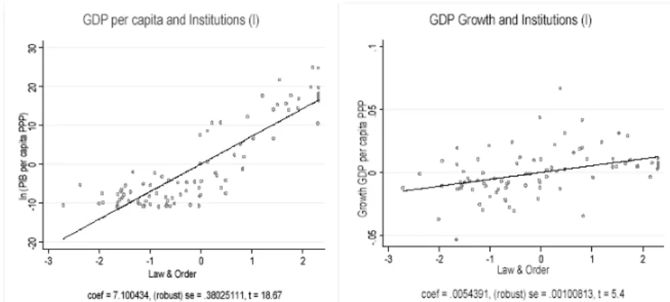
insti-tutions meaning that better instiinsti-tutions foster long run economic growth and countries with better institutions are the ones with higher per capita income levels. Figure 2 illustrate such evidence for our complete set of 91 countries where the proxy for institution (Law & Order) shows a positive and
statisti-cally significant coefficient when plotted against the log of per capita GDP
and the GDP growth rate. Regardless of such primary evidence it is necessary to investigate econometrically such relationship in both models using the
ade-quate techniques such as GMM System and Difference for growth models and
2SLS for models of per capita income levels. It is fair to say that the positive
coefficients reported in both graphs does not imply a specific causality from
institutions to GDP growth and per capita GDP levels since we might face reverse causality in the sense that countries with higher income levels and growth rates can create a better institutional environment, which is likely to happen in most cases.
Initially, it is necessary to address the role of institution and its definition. North (1990) definition of institutions is associated to the idea that institu-tions are the rules of the game in a society and it imposes constraints that shape human interaction. Acemoglu & Robinson (2004) highlights the rele-vance of institutions for improving economic growth and development, argu-ing that:
Economic institutions are important because they influence the structure of economic incentives in society, and without property rights, individuals will not have the incentive to invest in physical
or human capital or adopt more efficient technologies. Economic
institutions are also important because they help to allocate
re-1A historical look on the growth literature reveals that during the 1950s and 1960s growth theory was linked primarily to the neoclassical model developed by Ramsey (1928), Solow (1956), Swan (1956), Cass (1965) and Koopmans (1965). These models were based on the so-called con-vergence property and the idea is that economies with low per capita GDP will face higher growth rates given the assumption of diminishing capital returns. Since the 1980s, the concept of cap-ital in the neoclassical model has been expanded to incorporate not only physical capcap-ital but also human capital, as seen through the models developed by Lucas (1988) and Rebelo (1991), among others. Romer (1994) highlights the dilemma encountered by the theoretical and em-pirical growth literatures and the contribution of endogenous growth theory to understand the long-term growth, arguing that the main contribution of this approach is to provide a theory of technological progress, one of the central elements absent from the neoclassical growth model. The inclusion of a theory of technological change in the neoclassical framework is difficult, since
342 Vieira e Damasceno Economia Aplicada, v.15, n.3
Figure 1: Per Capita GDP and GDP Growth vs Institutions (Law)
sources to their most efficient uses, they determine who gets
prof-its, revenues and residual rights of control.
On the empirical evolution of the growth literature and the contribution of geography, integration and institutions, Rodrik et al. (2004) argues that:
Growth theory has traditionally focused on physical and human capital accumulation, and, in its endogenous growth variant, on technological change. But accumulation and technological change are at best proximate causes of economic growth. (. . . )
But why did some societies manage to accumulate and innovate
more rapidly than others? The three-fold classification offered
above – geography, integration, and institutions – allow us to or-ganize our thoughts on the “deeper” determinants of economic growth. These three are the factors that determine which societies will innovate and accumulate, and therefore develop, and which will not.
The following review of the literature will be divided into two sets. The first one deal with the empirical studies where the per capita GDP growth rate is the dependent variable, while the second one has the per capita GDP level
as the dependent variable since it is concerned with differences in such levels
across countries and not with their growth rates.
The evolution of the empirical growth literature using panel data goes back to the work developed by Barro et al. (1995) using data for more than one hundred countries from 1960 to 1990. The empirical results suggest that, for
a given level of real per capita income, the growth rate is positively affected by
the level of education and life expectancy, low fertility, lower government con-sumption, by maintaining the rule of law, lower inflation rate, improvement in the terms of trade, and negatively by the initial level of real per capita GDP. The inflation rate not only has a negative impact on real GDP growth in the long run, but also on the investment rate, but this result is statistically signif-icant when the economies with a history of high inflation are included in the
sample2.
Acemoglu & Robinson (2004) develops the empirical and theoretical case
where differences in economic institutions are the fundamental cause of diff
er-ences in economic development since there are different ways of organizing
societies in order to encourage innovation, to save for the future, to find better ways to improve knowledge and education, and to provide public goods.
Acemoglu et al. (2001) is a referential paper on addressing the endogene-ity problem of using proxies for institutions when examining and evaluating
difference in economic performance among countries. The paper uses diff
er-ences in mortality rates as an instrument to estimate the effect of institutions
on economic growth using 2SLS estimation, and the results are robust to
dif-ferent specifications, indicating the occurrence of significant effects of
insti-tutions on per capita income for a set of 64 countries. The main idea of the
model is to estimate the coefficients associated to variables (indexes) of
pro-tection to the risk of expropriation as a proxy for institutions. The argument is that countries with better institutions, with more secure property rights, and policies with less distortion, tend to invest more in physical and human
capital and usually have a more efficient use of such production factors in
or-der to achieve a higher level of income. The authors make clear that when using the mortality rate as an instrument for institutions, this is valid only if other variables that are correlated with the mortality rate are not related to the per capita income. The idea is that the instrument for institutions (mor-tality rate) should be an important factor to capture the variation observed in
the institutions, without having an effect on the growth rate.
Rodrik (1999) investigates the difference in growth rates for the periods
1960-75 and 1975-89 and the motivation of the study is to understand some issues and questions there are not a consensus in the growth literature such as: what are the crucial factors responsible for instability in the economic perfor-mance of developing countries; why countries that have a good economic per-formance in the 1960s and 1970s have had problems in the following decades;
why some countries were strongly but shortly affected by external volatility
in the second half of 1970 while others took a lot of time to recover from such external shocks; what are the main reasons underlying the process of
ex-pansion of the adverse effects of external shocks on the growth rate of many
economies.
The hypothesis investigated by Rodrik (1999) is that domestic social flicts are crucial to understand and answer the above questions as these con-flicts have a negative impact on productivity, besides being related to cases involving the postponement of policies associated to fiscal and relative prices
(real exchange rate and wages) adjustments. Another key aspect is the effect
that such conflicts have on the uncertainty (investment decision) of the econ-omy and the diversion of activities out of the production sector. The empirical analysis uses indicators of inequality, ethnic fragmentation, quality of govern-ment institutions, rule of law, democratic rights and social protection network to test RodriK’s hypothesis. The results indicate that countries that had the greatest reduction in the rate of GDP growth in 1975 were those where soci-ety is more fragmented and has fragile institutions. The degree of severity of
external shocks can be considered secondary in explaining the differences in
growth rates between countries, and once controlling for social conflicts and institutional quality, other factors (trade policies, government consumption,
ratio of debt / exports) have little explanatory power over such differences
con-344 Vieira e Damasceno Economia Aplicada, v.15, n.3
flict that ultimately is linked to the adoption of inadequate macroeconomic policies.
The second branch of the literature deals with empirical tests on the role of institutions and other factors in explaining why countries have such a huge
difference in per capita income levels. Hall & Jones (1999) is one of the
pio-neers in examining the issue of why output per capita is so different across
countries using a large set of countries. The main goal is to explain changes in long-run economic performance focusing directly in the investigation of cross-section analysis for income levels. One of the main empirical findings
is that differences in capital accumulation, productivity and ultimately in per
capita income is due to differences in institutions and government policies.
The authors call this as social infrastructure and considered it as endogenous, which requires finding variables that are good instruments (location and
lan-guage) in order to overcome problems such as coefficient bias in the presence
of endogenous variables3. The authors emphasize that productivity is crucial
to understand such differences in income levels. The goal is to answer two
main questions: Why there is a significant difference in investments in
phys-ical and human capital? Why there is an important productivity difference
across countries?
In order to answer these questions, Hall & Jones (1999) argue that long run economic performance of a country is primarily determined by social
in-frastructure, meaning that differences in capital accumulation, productivity
and ultimately in per capita output are related to different levels of social
in-frastructure. Examining 127 countries the authors found a close and positive relation between per capita output and social infrastructure. After controlling for endogeneity of social infrastructure (institutions and government policies)
they still find evidence that most of differences in long-run economic
per-formance is due to differences in social infrastructure across countries. The
estimated coefficient for output per capita and productivity is 0.60 and the
correlation between the differences for the two series in log is 0.89. Most of
the differences in output per capita are due to productivity by a factor of 8.3
against human capital with 2.2 and capital intensity with 1.8 when compar-ing the five highest and lowest countries in terms of output per capita, which
are different by more than 30 times for this set of countries.
The estimation of the social infrastructure index (SI) by Hall & Jones (1999) uses a combination of two indexes to construct the proxy for SI. One is the in-dex of government antidiversion policies (GADP) based on data from the Polit-ical Risk Service (130 countries and 24 categories) and the authors select five categories: law and order; bureaucracy quality; corruption; risk of expropria-tion and government repudiaexpropria-tion of contracts, each of them as average for the period of 1986-95. The second index tries to capture the degree of openness to trade and it draws from the data developed by Sachs & Warner (1995) and it
varies from 0 to 1 according to criteria such as: level of nontariffbarriers;
aver-age tariffrates; black market premium; country classified as non-socialist; and
absence of government as a monopolist for major exports. The final proxy for SI is given by the sum of GADP and the openness index and the instruments used captures geography characteristics (distance from the equator), the
West-3Studies such as Weil et al. (1992) was crucial in setting an empirical agenda to investigate dif-ferences in per capita income levels across countries based on differences in human and physical
ern European influence (primary spoken language) and the (log) predicted trade share of the economy constructed by Frankel & Romer (1999). The
esti-mated model for output per capita shows that the estiesti-mated coefficient for
so-cial infrastructure is positive (for the main specification ˆβSI = 5.14 with four
instruments) and statistically significant for all specifications. The authors conclude after some robustness tests that taking into account elements such as geography (distance from the equator) and Western influence (language),
differences in social infrastructure determines (cause) large differences in per
capita income across countries.
Other works such as the one developed by Easterly & Levine (2003) is
focused on understanding differences in per capita income across countries.
They develop an analysis first reviewing the empirical literature / theories of how geography, institutions, and policy influence economic development
and so the disparity in income levels. Thegeography / endowment hypothesis
argues that environment has a direct impact on the quality of land, labor, and
production technologies, while the institution viewis based on the idea that
the environment’s main impact on economic development operates through
institutions. Thepolicy viewtries to minimize the relevance of tropics, germs,
and crops as a fundamental determinant of differences in economic
develop-ment and income level by arguing that economic policies and institutions are a result of current knowledge and political forces. Within this perspective, to change income levels it is necessary to understand each country policies and institutions. Ultimately, the authors seek to empirically address which
of these three views / theories are more adequate to explain differences in
income levels across countries4.
Easterly & Levine (2003) uses settler mortality as an indicator of endow-ments to test the geography and the institutions hypotheses and other con-trol variables such as: latitude, dummies for crops / minerals, landlocked, a measure for openness (Frankel & Romer 1999), real exchange rate overvalu-ation and inflovervalu-ation to address the policy view, and six indexes for quality of institutions draw from Kaufmann et al. (2008) to capture the relevance of in-stitutions in a per capita income model. The authors also use other control variables such as ethno linguistic diversity, religion and French legal origin.
The initial step was to estimate a model for a sample of 72 countries by OLS with heteroskedasticity consistent standard errors for the log of the per capita GDP on the endowment variables and the results indicate that endow-ments explain cross-country variation in per capita income. The next step
4The geography/endowment hypothesis is associated to different studies such as Sachs &
Warner (1995), Sachs & Warner (1997), Bloom & Sachs (1998) and O’Neill (2001), arguing for the presence of direct effects of tropics, germs, and crops on development. The institutions
hy-pothesis relates the effect of tropics, germs, and crops through institutions and can be associated
to works such as Hall & Jones (1999) who uses institutional quality as one component of social infrastructure which is crucial to explain differences in productivity, allowing for the use of
346 Vieira e Damasceno Economia Aplicada, v.15, n.3
was to run an OLS model and check if endowments help to explain
cross-country differences in institutional development and the results indicate that
variables like settler mortality and natural resources (germs and crops) are the dominant forces to understand institutional development. Up to this point the Easterly & Levine (2003) have found evidence that endowments have an impact on economic and institutional development. Following this result, the authors estimate a 2SLS model for the log of per capita GDP using four instru-ments (settler mortality, latitude, landlocked and crops/minerals) in the first stage estimation, and institutions index, French legal origin, religion, ethno linguistic diversity and oil as exogenous variables in the second stage
estima-tion. The estimated coefficients for the institution indexes are all positive and
statistically significant and the overidentification tests were not rejected indi-cating that the set of instruments are valid. The final estimated model treats macroeconomic policy variables (inflation, openness and real exchange rate overvaluation) as endogenous using 2SLS and the evidence suggests that such
policies do not explain differences in per capita income after taking into
ac-count the impact of institutions on income levels. The estimated coefficients
for the institution index are all positive and statistically significant.
The empirical evidence found by Easterly & Levine (2003) suggests that endowments (tropics, germs, and crops) have an impact on per capita income
through institutions but not a direct effect, which is a support for the
institu-tion view but not for the geography one. The same is true for what they call policies variables which has no impact on development when controlling for
institutions, in other words, institutions rule differences in per capita income
levels across countries. Such empirical results are hand to hand with the work of Acemoglu et al. (2001).
Acemoglu & Robinson (2004) review what is called the geography
hypoth-esis as an alternative to explain difference in economic performance among
countries and the main idea is to focus on the role of physical and
geographi-cal environment. This approach emphasizes differences in geography, climate
and ecology as fundamental in understanding how preferences and the
oppor-tunity set of individual economic agents in different societies. The geography
hypothesis can be divided into three versions. The first one highlights how
climate may be an important factor of work effort, incentives, or productivity.
The second one argues that geography may determine the technology avail-able to a society, especially in agriculture, while the last one is based on the idea that infectious disease is costly and more likely to happen in the tropics than in the temperate zones, which can mitigate economic performance over time (Sachs 2000).
One can say that there is a clear disagreement among the role played by
geography in explaining differences in per capita income levels. Sachs (2003)
is an example of studies that do not agree with others such as Acemoglu et al. (2001), Easterly & Levine (2003) and Rodrik et al. (2004) on the proposition
that the role of geography in explaining cross-country differences in per
in-come is secondary and operates mainly through institutions. According to the author per capita income, economic growth, and other economic and demo-graphic dimensions are strongly correlated with variables associated to geog-raphy and ecology, including climate zone, disease ecology, and distance from the coast. The variable used to corroborate his argument is malaria
trans-mission, which is strongly affected by ecological conditions and has a direct
Rodrik et al. (2004) empirically investigates the contribution of
institu-tions, geography and trade in explaining differences in per capita income
across countries and the evidence suggests the predominance of institutions
over geography and trade using different instruments. The authors argue that
integration to the world economy and the quality of institutions should be
treated as endogenous since they affect each other and are affected by
geo-graphical variables and by income levels. Dealing with this means to take into account endogeneity and reverse causality issues in estimating a cross country income model.
The main empirical evidence found by Rodrik et al. (2004) is that once
in-stitutions are part of the regression (2SLS), integration has no direct effect on
per capita income, while geography measures have at best only weak direct ef-fects even though they are important to understand the quality of institutions. Trade does not reveal to be statistically significant once institutions are con-trolled for and it seems to have an unexpected negative sign. The estimated
coefficients for the measure of property rights and the rule of law are positive
and statistically significant. The authors also found similar evidence to East-erly & Levine (2003) that geography has a significant impact on the quality
of institutions and this is the channel through which it affects income levels.
In the preferred model specification (settler mortality as instrument for insti-tutions quality) developed by Rodrik et al. (2004) it was possible to account for half of the variance in cross country incomes and trade and distance from the equator are not statistically significant. Comparing the estimated coef-ficients (table 2 and OLS) for institutions (rule of law), geography (distance from the equator) and integration (log of trade to GDP) after they have been standardized in order to be comparable, the results for the log of GDP per
capita reveals that the coefficient for institutions is positive and statistically
significant and greater than the coefficient for geography (positive and
signif-icant), which is greater than the estimated coefficient for integration (positive
but not significant). The 2SLS estimation reported on table 3 reveals on the
preferred specification (column 6) that the coefficient for institutions is
pos-itive (1.98) and statistically significant, while the coefficients for geography
(−0.72) and integration (−0.31) are not significant and the latter has an
unex-pected sign.
The main criticism stated by Sachs (2003) with respect to the institutions rule argument is that there are specification problems in the model and how they test the primacy of institutions. The first specification problem is associ-ated to the use of a static rather than a dynamic model for per capita income and the author argues that it is more likely that the quality of institutions in a
given time period will affect the growth rate and not the income level but the
three mentioned studies are concerned in explaining differences in per capita
income and not in growth rates across countries. Other than this, Sachs (2003)
argues that differences in income levels should not be explained by only a few
348 Vieira e Damasceno Economia Aplicada, v.15, n.3
Regarding the use of indexes of institutional quality based on surveys of foreign and domestic investors (Rule of Law, Corruption, Investment Profile and Bureaucracy) Rodrik et al. (2004) states that such indexes are able to cap-ture investor’s perceptions but not exactly which are the rules governing these institutions, which is a limitation and future research on growth disparities will have to deal with this. It is also necessary to distinguish between stimulat-ing and sustainstimulat-ing economic growth and better and more reliable institutions are more important for the latter than to the former meaning that developing countries can boost initial growth with some minor changes in their institu-tional environment.
3
Institutions and
GDP
per capita Level: Empirical Evidence
This section summarizes methodological aspects of using the two stages least
square (2SLS) estimation method for models of cross country income diff
er-ences and reports the estimation results on tables 1 and 2.
3.1 Empirical Methodology
This section of the paper has two goals. First, specify the 2SLS estimation
pro-cedures since it is widely used in the cross section models of differences in per
capita income across countries. Second, compare the estimated coefficients
for different sets of countries using institutions, geography, integration and
instrumental variables.
The cross section empirical studies on per capita income differences across
countries are almost always based on the use of 2SLS estimation since this is the core instrument when dealing with endogeneity problems as it happens with the inclusion of institutions in this kind of model.
Considering the following model for a dependent variable (y) on a single
regressor (x):
yi=βxi+ui. (1)
Assuming that the regressor (x) is endogenous, the OLS estimation is not valid
since it violates the assumption required for consistency that the error term
(u) is not correlated to the regressors (Cov(x, u) = 0) and the instrumental
variable (IV) approach deals with this by selecting new variables (z) that are
highly correlated to the regressors (Cov(z, x),0) but not with the error term
(Cov(z, u) = 0).
The 2SLS estimation is based on a two stage procedure where the first implements an OLS estimation of the endogenous variable (proxy for institu-tions) as the dependent variable as a function of exogenous variables and the
new set of instruments (z) and this is called the reduced form equation. The
second stage is the OLS regression of the dependent variable of the original model (log of per capita GDP) on the exogenous variables and the replace-ment of endogenous regressors by predictions from the first stage. One ad-vantage of the 2SLS estimation is that in the presence of independent and
homocedastic errors it is the most efficient estimator but since this is not an
easy assumption, we use the correction for heteroskedasticity in our estimates
(tables 1 and 1).5
heteroskedastic-3.2 Empirical Results
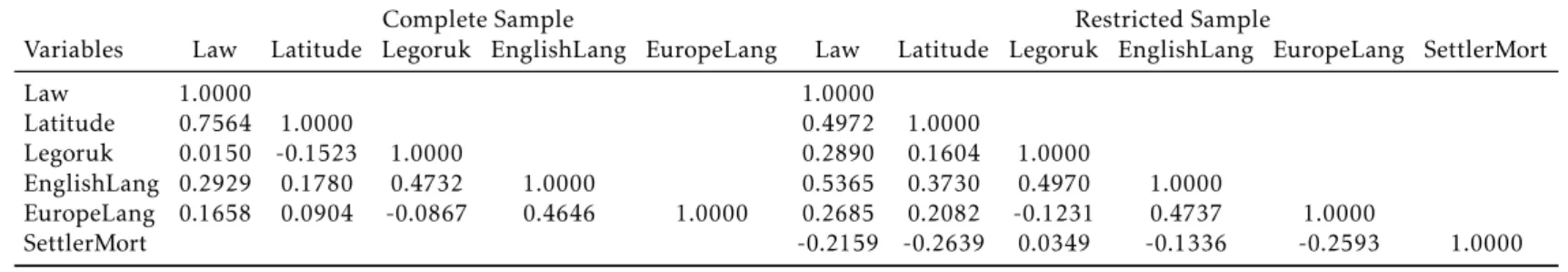
First of all, it should be emphasized that the set of instruments used in the 2SLS estimation when dealing with endogeneity of institutions (Law) is Set-tlerMort, Legoruk, EnglishLang, and EuropeLang, where for integration (Trade) we use the index developed by Frankel & Romer (1999) to capture perceived
integration.6
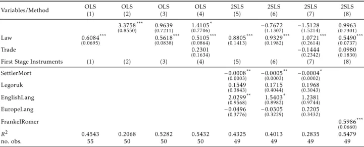
The estimation of the cross-section models of per capita GDP levels for the complete sample (91 countries) using 2SLS is reported on table 1. The
2SLS estimated models (columns 5, 6, 7 and 8) show that the coefficients for
institutions (Law) are positive and statistically significant in all four models. It is necessary to interpret this result with some caution since models (5) and (6) that are over-identified have overidentification tests that reject the null at 5%, and so the instruments are not valid. Comparing the 2SLS and the
OLS coefficients for Law one can see that the 2SLS estimation provides higher
estimates. Geography (Latitude) has a negative (unexpected) coefficient for
models (6) and (7) but in both cases it is not statistically significant while in
model (8) it has a positive and significant coefficient. Trade (integration) is not
statistically significant in the two 2SLS estimation (7 and 8) regardless if it is considered as exogenous (7) or treated as endogenous (8) and instrumented by FrankelRomer index of perceived trade openness.
The next step is to estimate the same models from table 1 but now for a restricted sample which includes countries in our sample with data for Settler Mortality, which is the instrumental variable used by Acemoglu et al. (2001).
The only difference is that on table 2, settler mortality was used as an
instru-ment while in table 1 it was not.
The 2SLS estimated models from table 2 (columns 5, 6, 7 and 8) show that
ity correction, which is based on a weighting matrix that it different from the one used by 2SLS
estimation. One of the problems associated to 2SLS estimation is how to avoid the use of weak instruments since they will result in less precise coefficients due to high standard errors (lower
t-statistics) and the occurrence of finite sample bias (the IV estimator is not centered on the true populational coefficient). See Cameron & Trivedi (2008) chapter 6 for further details on 2SLM
and OGMM. The paper uses overidentification tests with the estat overid command for Stata 10.0 and the estat firststage command to evaluate the presence of weak instruments (F-stat of first stage). Table A.4 of the appendix reports additional estimation such as the OGMM for the cross-section models in order to have a broader range of coefficient estimates and to compare them with
the 2SLS.
35
0
V
ie
ir
a
e
D
am
as
ce
n
o
E
co
n
om
ia
A
p
lic
ad
a,
v.1
5
,
n
.3
Table 1: Cross-Section Real Per Capita GDP Models - Complete Sample
Variables/Method OLS(1) OLS(2) OLS(3) OLS(4) 2SLS(5) 2SLS(6) 2SLS(7) 2SLS(8)
Latitude 4.2889
(0.4120)
*** 1.2890 (0.5221)
** 1.4959 (0.5160)
*** −0.9645
(1.5246) −(12..16069819) (01..33484893)
***
Law 0.7120
(0.0442)
*** 0.5577
(0.0741)
*** 0.5227 (0.0733)
*** 0.8944 (0.1538)
*** 0.9620 (0.2752)
*** 1.1785 (0.3555)
*** 0.5394 (0.0687)
***
Trade 0.1596
(0.1306) −(00..23432638) (00..11801574)
First Stage Instruments (1) (2) (3) (4) (5) (6) (7) (8)
Legoruk −0.5134
(0.3479) (00..30582995) (00..26202410)
EnglishLang 2.0639
(0.8090)
** 0.4052
(0.6210) (00..31096826)
EuropeLang −0.0912
(0.4521) (00..23692355) (00..40312470)
FrankelRomer 0.5396
(0.0559) ***
R2 0.6487 0.4974 0.6794 0.6840 0.6069 0.5875 0.4690 0.6857
no. obs. 91 82 82 82 81 81 81 81
F Stat First Stage (p-value) 0.0303 0.0000 0.0000 0.0000
Test Overid (p-value) 0.0372 0.0411 0.1128
Test Endogenous (p-value) 0.0702 0.0618 0.0053 0.7150
the coefficients for institutions (Law) are positive and statistically significant
in all four models. In the same way when we present the results from table 1, it is necessary to interpret this result with some caution since models(5),(6) and(7) that are over-identified have overidentification tests that reject the null at 5% and so the set of instruments are not valid. Geography (Latitude) is not statistically significant in any of the three models using 2SLS and it has an unexpected negative sign in models 6 and 7. Trade (integration) is not statistically significant in the two 2SLS estimation (7 and 8) regardless if it is considered as exogenous(7) or treated as endogenous(8) and instrumented by
the index constructed by Frankel & Romer (1999).7
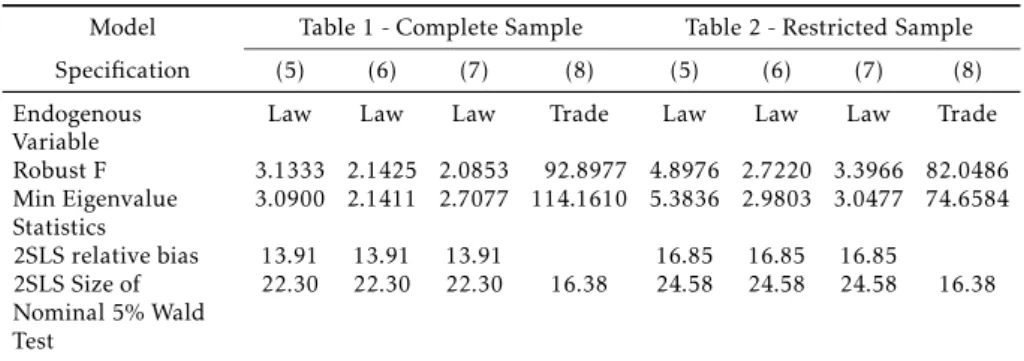
After the cross-section estimation reported on tables 1 and 2 the paper de-velops an empirical investigation on the issue of weak instruments based on
a set of tests reported in table 3. 8 Stock & Yogo (2005) developed two tests
for weak instruments and following Cameron & Trivedi (2008) we implement these tests for the cross-section analysis. Basically the tests have a null hypoth-esis that the instruments are weak against the alternative that they are strong and the idea is to look at the Robust F statistics for joint significance of instru-ments in the first-stage regression and the minimum eigenvalue statstics and compare these with the critical values from Stock & Yogo (2005) tables. A rule of thumb for the F statistics is that if it is greater than 10 we can say that it is possible to reject the null of weak instruments.
Examining table 3 we can see that the Robust F statistics do not reject the null for models (5), (6) and (7) for the complete and restricted sample when Law is the instrumented variable so there is evidence of weak instruments, except for model (8) in both samples when Trade is included as endogenous variable in the model. Once we look at the minimum eigenvalue statistics there is evidence of weak instruments for all models except when Trade is treated as endogenous, model (8) in both samples.
Summarizing the results for the cross-country differences in per capita
in-come levels it is fair to say that there are some mixed evidences regarding
the role of institutions (Law) since all the estimated coefficients are positive
and statistically significant but there is evidence that theinstruments are not valid and even if they are we do have weak instruments for the most estimated models.Integration (Trade) and Geography (Latitude) do not seem to play a
di-rect and significant role on explaining differences in per capita income levels
across countries when modeling institutional variables (Law) as endogenous or even when integration (Trade) is considered endogenous.
4
Institutions and GDP per capita Growth: Empirical Evidence
This section of the paper presents some methodological issues on panel data estimation for long run growth models and the use of the generalized method
of moments (GMM) reporting on table 4 and 5 the estimated coefficients for
the complete sample and for developing countries.
7Examining the results from table 4A of the appendix for a comparison of different estimation
methods we can see that there is a significant variation on the estimated coefficients when using
the Jacknife IV (JIVE) and the LIML estimators that are asymptotically equivalent to 2SLS but may have better finite sample properties than 2SLS. The estimated coefficients for 2SLS and OGMM
are much more similar for both complete and restricted samples.
35 2 V ie ir a e D am as ce n o E co n om ia A p lic ad a, v.1 5 , n .3
Table 2: Cross-Section Real Per Capita GDP Models - Restricted Sample
Variables/Method OLS(1) OLS(2) OLS(3) OLS(4) 2SLS(5) 2SLS(6) 2SLS(7) 2SLS(8)
3.3758 (0.8550)
*** 0.9639
(0.7211) (01..41057706)
* −0.7672
(1.1307) −(11..51285214) 0(0..99637301)
Law 0.6084
(0.0695)
*** 0.5618
(0.0838)
*** 0.5105 (0.0864)
*** 0.8805 (0.1413)
*** 0.9329 (0.1982)
*** 1.0721 (0.2614)
*** 0.5490 (0.0737)
***
Trade 0.2301
(0.1634)
−0.1444
(0.2342) 0(0..09801830)
First Stage Instruments (1) (2) (3) (4) (5) (6) (7) (8)
SettlerMort −0.0008
(0.0003)
** −0.0005 (0.0003)
** −0.0004 (0.0002) *
Legoruk 0.1549
(0.3843) (00..17154044) (00..19683043)
EnglishLang 2.0299
(0.9568)
** 1.5403 (0.8982)
* 1.2381 (0.9744)
EuropeLang −0.0496
(0.3776) −(00..03053229) (00..22053432)
FrankelRomer 0.5986
(0.0660) ***
R2 0.4543 0.2068 0.5282 0.5432 0.4325 0.4013 0.2835 0.5479
no. obs. 55 50 50 50 49 49 49 49
Table 3: Testing for Weak Instruments
Model Table 1 - Complete Sample Table 2 - Restricted Sample
Specification (5) (6) (7) (8) (5) (6) (7) (8)
Endogenous
Variable Law Law Law Trade Law Law Law Trade
Robust F 3.1333 2.1425 2.0853 92.8977 4.8976 2.7220 3.3966 82.0486 Min Eigenvalue
Statistics 3.0900 2.1411 2.7077 114.1610 5.3836 2.9803 3.0477 74.6584
2SLS relative bias 13.91 13.91 13.91 16.85 16.85 16.85
2SLS Size of Nominal 5% Wald Test
22.30 22.30 22.30 16.38 24.58 24.58 24.58 16.38
Note: 2SLS relative bias is 5% critical value and 2SLS Size of Nominal 5% Wald Test is 10%
critical value.
4.1 Empirical Methodology
This section of the study aims to specify the methodology of panel data anal-ysis using GMM estimation to be used in the econometric analanal-ysis, specifying the growth models to be estimated, the number of countries in the sample and the explanatory variables.
The study uses a dynamic panel data model specification and the motiva-tion for the use of this methodology is the possibility to take into account the following: (i) the time series dimension of the data, (ii) non observable
coun-try specific effects; (iii) inclusion of lagged dependent variable among the
ex-planatory variables, and (iv) the possibility that all exex-planatory variables are endogenous.
The standard approach on panel data starts with the assumption that the growth rate path is consistent with the following procedure:
yi,t−yi,t−1= (α−1)yi,t−1+β′Xi,t+ηi+εi,t, i= 1, . . . , N , t= 2, . . . , T , (2)
wherey is the natural log of per capita real GDP,X represents the set of
ex-planatory variables, η is a non-observable and country specific term, εis a
random term and the subscripts i and t refers to country and time,
respec-tively9.
It should be noted that the time specific effect allows to control the
in-ternational conditions that change over time and ultimately affect the growth
performance of countries in the sample, while the non observable country
spe-cific effect (η) incorporates factors that influence the growth of per capita GDP
and are potentially correlated with the explanatory variables.What character-izes the dynamic relationship is the presence of lagged dependent variable as one of the explanatory variables, which is evident once we rewrite equation (2) as:
yi,t=αyi,t−1+β ′
Xi,t+ηi+εi,t. (3)
The elimination of the country specific and the non observable term (η) is
obtained once we apply first difference to equation (3):
yi,t−yi,t−1=α(yi,t−1−yi,t−q2) +β′(Xi,t−Xi,t−1) + (εi,t−εi,t−1) (4)
354 Vieira e Damasceno Economia Aplicada, v.15, n.3
The use of instruments is required to deal with the possible endogeneity of the explanatory variables and the correlation between the new term of error, εi,t−εi,t−1, and the lagged dependent variable,yi,t−1−yi,t−2. Under the
assump-tions that the error term (ε) is not serially correlated and the explanatory
vari-ables (X) are weakly exogenous, lagged values of the explanatory variables can
be used as instruments, as specified under the following moment conditions:
E
yi,t−s· εi,t−εi,t−1
= 0 for all
s≥2;t= 3, . . . T (5)
E
Xi, t−S· εi,t−εi,t−1
= 0 for all
s≥2;t= 3, . . . , T (6)
The GMM estimator based on the moment conditions (5) and (6) is called
Difference GMM and we call this GMM-DIFF throughout the paper. There are
statistical problems associated with the use of GMM-DIFF: statistically, when
the regressors in equation (4) are persistent, lagged levels ofXandyare weak
instruments. The use of weak instruments asymptotically implies that the
variance of the coefficient increases and in small samples the coefficients can
be bias. To reduce the potential bias and inaccuracy associated with the use of DIFF-GMM estimator, Arellano & Bover (1995) and Blundell & Bond (1998)
develop a system of regressions in differences and levels. The instruments for
the regression in differences are the lagged levels of the explanatory variables,
moment conditions (5) and (6). The instruments for the regression in levels
are the lagged differences of explanatory variables. These are appropriate
in-struments under an additional assumption, that is, although there may be correlation between the levels of explanatory variables and the country
spe-cific effect (η) in equation (3), there is no correlation between those variables
in differences and the country specific effect (η). This can be represented as:
Ehyi,t+p.ηi
i
=E[yi,t+q.ηi]
and
EhXi,t+p.ηi
i
=E[Xi,t+q.ηi], for allpandq. (7)
The moment conditions for the regression in levels, which is the second part of the system, are:
E(
yi,t−s−yi, t−s−1).(ηi+εi,t)= 0, fors= 1. (8)
E(
Xi,t−s−Xi, t−s−1).(ηi+εi,t)= 0, fors= 1 (9)
The GMM estimator based on the moment conditions (5), (6), (8) and (9) is called System GMM or GMM-SYST throughout the paper. The consistency of the GMM estimator depends on the validity of the moment conditions. To such extent it will be considered two specification tests based on Arellano & Bond (1991), and Arellano & Bover (1995) and Blundell & Bond (1998):(i) Hansen test is a test of overidentifying restrictions and the joint null hypothe-sis is that the instruments are valid, i.e., uncorrelated with the error term, and that the excluded instruments are correctly excluded from the estimated equa-tion; (ii) and the Arellano-Bond test which tests the hypothesis of no second order serial correlation in the error term.
Recently, studies such as Roodman (2009a) and Roodman (2009b), develop
and System GMM. The author discusses the symptoms of instrument prolif-eration showing that as the time dimension increases, the number of instru-ments can be too large compared to the sample size and the outcome is that some asymptotic results and specification tests are not valid. Too many instru-ments can over fit endogenous variables and fail to expunge their endogenous
components, resulting in biased coefficients. Another argument is that the
Hansen and Difference-in-Hansen tests can be weak when using the Diff
er-ence GMM and System GMM in the preser-ence of overidentification.
In order to deal with too many instruments, Roodman (2009a) suggest the
use of thecollapsesuboption for thextabond2command in Stata. The author
develops an analysis on the existence of two techniques to limit the number of
instruments generated in difference and system GMM. The first one is based
on the idea of using only certain lags instead of all available lags for instru-ments and in this case the number of instruinstru-ments per period is limited in
such a way that it is linear in T. The use of theCollapsesuboption is part of the
second approach to reduce the number of instruments and it is the one rec-ommended by the author. The main idea is to combine instruments through addition into smaller sets, without dropping any lags as the first technique
does. TheCollapsesuboption implies the creation of one instrument for each
variable and lag distance, rather than one for each time period, variable, and lag distance, where the final outcome is to divide the GMM-style moment con-ditions into groups and sums the concon-ditions in each group to form a smaller set of conditions. At the end, we have a set of collapsed instruments where one is made for each lag distance, with zero substituted for any missing values
and making the number of instruments linear in T.10
The panel data model is estimated for the complete sample (91 countries) and for developing countries over the period 1980-2004. The data used are transformed and are based on averages for non-overlapping periods of five years (1980-1984, 1985-1989, 1990-1994, 1995-1999, 2000-2004), so that there are five data entries for each country for each variable in the sample. The
rea-son for using five year average data is to minimize the business cyclical effects
and the error term to be less likely to face autocorrelation problems (see Islam (1995)). There is no data for all countries, time and variables, so the estimated panel is an unbalanced one. The variables used in the econometric estimation are reported on table A.1 of the appendix, where the variables were in the logarithmic form except for the time dummies and the indexes of institution quality.
4.2 Empirical Results
The analysis of table 4 reveals that the coefficient for institution (Law) is
pos-itive in for all models and statistically significant only when using the GMM-SYST for the complete sample in a more parsimonious specification (without Credit, Pop and TermsTrade) and this result stands in three out of four (5, 6
and 8) estimation models for developing countries11. The results also suggest
10A more detailed presentation including matrix notation can be found in Roodman (2009a), p.148-149. See also Baltagi (2008) for further empirical examples using the collapse command.
11The results for the AR(2), Hansen and Hansen Difftests indicate that we are able to reject the
null hypothesis meaning that there is no second order autocorrelation and the instruments are valid, with only one exception for the Hansen Difftest in model specification (1) using
356 Vieira e Damasceno Economia Aplicada, v.15, n.3
that Gov (government consumption) has a negative and statistically
signifi-cant coefficient in all estimated models, suggesting a robust role played by
such policy variable, meaning that countries with more fiscal discipline
bene-fit over time in terms of fostering economic growth12.
Some minor evidence of significance was found for Educ only for model(2) using GMM-SYST, for Credit in models (4) and (8) using GMM-DIFF but only
at 10% and for Pop in model (2) using the GMM-SYST. The estimated coeffi
-cients for the integration to the world economy (Trade), macroeconomic sta-bility (Inf) and Terms of Trade were not statistically significant in any model
specification13.
After all one can say that the empirical result for the long-run per capita GDP growth models suggest that there are mixed evidence for the role of institutions (Law) in fostering economic growth and the GMM-SYST is the one that is more likely to capture such role and the quality of institutions seems to be more relevant for developing countries. Another lesson to be draw from the estimated growth models is that fiscal discipline (policy variable), measured by government consumption / GDP, plays a crucial role in stimulating long-run growth.
Recent work such as Roodman (2009a) and Roodman (2009b) and Bazzi
& Clements (2009) emphasize the need for a deeper investigation on weak in-struments for cross-section and instrument proliferation for panel data anal-ysis. Since for one model (1) the overidentification tests from table 4 suggest the existence of poor instruments and given the use of a significant number of instruments, especially for the System GMM, we have estimated the same model using a reduced number of instruments (collapse command in Stata) and the results are reported on table 5.
Comparing the results with fewer instruments (table 5) with the ones from table 4 one can see that for the complete sample (columns 1, 2 3 and 4)
in-stitutions (Law) has a positive and significant coefficient in model (4) and
only at 10%, which is different from previous estimation when System-GMM
was more likely to capture such role for institutions in the complete sample and developing countries were more likely to face significant estimated ficients. Government spending and population growth have significant coef-ficients for the System GMM estimation using the complete sample, while for
the Difference GMM model (4), years of schooling (Educ) and credit are
sig-nificant but with unexpected signs. For developing countries (columns 5 to
8) government spending is the only variable with significant coefficient for all
models and population growth for System GMM. There is no significant
co-efficient for institutions (Law) regardless of the estimation method or model
specification which is a contrasting result with the one from previous estima-tion where in three out of four models for developing countries Law has a
positive and significant coefficient. Such results can be seen as additional
em-pirical evidence that there is no emem-pirical support for the argument that
insti-12Sala-I-Martin & X. (1990) develops a theoretical and empirical investigation on the contri-bution of government spending to growth considering not only government consumption, as we have done in our paper, but also government investment (infrastructure) suggesting a possibility that government investment can foster economic growth.
13Conditional convergence (negative coefficient for Yinitial) is observed for all estimated mod-els except for model (5) and most coefficients are statistically significant except for models (1)
In st itu tio n s fo r In co m e an d G ro w th M od els 35 7
Variables/Method Complete Sample Developing Countries
System System Diff Diff System System Diff Diff
(1) (2) (3) (4) (5) (6) (7) (8)
0.1027
(0.0883) 0(0..15860814)
* −0.0967
(0.0597) −0(0..14980824) (00..15660813) 0(0..05581007)
* −0.1275 (0.0708)
* −0.1305 (0.0918) Yinicial −0.0075
(0.0248) −0(0..05520212)
*** −0.2927 (0.0775)
*** −0.2461 (0.0835)
*** 0.0160
(0.0315) −0(0..04560264)
* −0.2147 (0.0876)
** −0.2401 (0.0818)
***
Educ 0.0053
(0.0459) 0(0..09820518)
* −0.0068 (0.1126)
−0.2367
(0.1462) (00..02660547) (00..08820595) (00..16261994)
−0.1870 (0.2205)
Law 0.0371
(0.0120)
*** 0.0250
(0.0160) (00..01610125) (00..02360165) (00..02400131)
* 0.0386 (0.0152)
** 0.0119
(0.0149) (00..04360237) *
Trade 0.0061
(0.0229) −0(0..01930199) (00..05710610) 0(0..02010961) −(00..01250221) −0(0..04350292) (00..12650809) (00..06200824)
Gov −0.1037
(0.0407)
** −0.1226 (0.0428)
*** −0.1215 (0.0569)
** −0.1657 (0.0515)
*** −0.1039 (0.0415)
** −0.0845 (0.0381)
** −0.1515 (0.0641)
** −0.1449 (0.0753)
*
Inf 0.0017
(0.0103) −0(0..00960095) −(00..00700055) −0(0..01020113) −(00..00000086) −0(0..00920145) −(00..00690103) −(00..00960105)
Credit −0.0224
(0.0182) −0(0..04980283)
* 0.0066
(0.0348) −(00..08410490) *
Pop −0.0539
(0.0188)
*** −0.0216
(0.0145) −0(0..04290308)
−0.0111 (0.0257)
Terms Trade 0.0335
(0.0353) 0(0..00570394) (00..06150519) (00..00630257)
AR (2) 0.170 0.468 0.925 0.654 0.663 0.900 0.767 0.546
Hansen 0.208 0.879 0.335 0.284 0.951 1.000 0.385 0.800
Hansen Diff 0.020 1.000 0.991 1.000
No. instruments 72 91 48 61 72 91 48 61
No. obs. 306 264 224 191 220 190 160 137
Note: Dependent Variable is real GDP per capita growth, PPP basis (Growthppp). Yinitial, Educ, Inf, Gov, Trade and Credit are in log. All estimations are Two-Step and standard errors are corrected by the Windmeijer (2005) procedure. All estimations use the xtabond2 (Roodman 2009a) command for Stata 10. AR(2), Hansen Test and Diff. Hansen Test reports thep-values. System
35 8 V ie ir a e D am as ce n o E co n om ia A p lic ad a, v.1 5 , n .3
Table 5: Real GDP Growth Models: Dealing With Instrument Proliferation
Complete Sample Developing Countries
Variables/Method System System Diff Diff System System Diff Diff
(1) (2) (3) (4) (5) (6) (7) (8)
Growtht-1 0.0754
(0.1126) 0(0..08131134) −(00..08750821) −0(0..23181242)
* 0.1501 (0.0795)
* 0.0186
(0.0964) −(00..00431112) −(00..13551638) Yinicial 0.0373
(0.0361) −(00..01180516) −(00..42231648)
*** −0.2130 (0.0738)
*** 0.0880 (0.0440)
** −0.0354
(0.0702) −(00..15891530)
−0.2408 (0.1047) **
Educ 0.0062
(0.0746) 0(0..09310918) −(00..09721271) −0(0..65262239)
*** −0.0510
(0.0843) 0(0..13021112) −(00..20512207) −(00..39873445)
Law 0.0073
(0.0179)
−0.0026
(0.0203) (00..00730138) 0(0..04230231)
* 0.0148
(0.0193) 0(0..02270178)
−0.0046
(0.0247) (00..01240347)
Trade −0.0525
(0.0732) −0(0..06680602) (00..03401184) 0(0..07701434) −(00..04040639) −0(0..07920512) (00..17131187) (00..19181344)
Gov −0.2650
(0.0725)
*** −0.2629 (0.1115)
** −0.0875 (0.0798)
−0.1507 (0.0947)
−0.2607 (0.0631)
*** −0.2207 (0.0819)
*** −0.2160 (0.0814)
*** −0.2094 (0.1027) **
Inf −0.0230
(0.0157) −0(0..02600175) −(00..00640092) −0(0..01160128) −(00..01060148) −0(0..01800158) −(00..00970150) −(00..00880167)
Credit −0.0159
(0.0475) −0(0..13150548)
** 0.0207
(0.0536) −(00..07040707)
Pop −0.0720
(0.0229)
*** −0.0296
(0.0315)
−0.0958 (0.0406)
** −0.0035
(0.0378)
Terms Trade 0.0302
(0.0500) 0(0..01670533) (00..05470670) (00..00790334)
AR(2) 0.138 0.407 0.763 0.160 0.701 0.743 0.626 0.610
Hansen 0.174 0.154 0.254 0.196 0.756 0.172 0.095 0.105
Hansen Diff 0.032 0.152 0.442 0.385
No. instruments 34 43 25 32 34 43 25 32
No. obs. 306 264 224 191 220 190 160 137
Note: Dependent Variable is real GDP per capita growth, PPP basis (Growthppp). Yinitial, Educ, Inf, Gov, Trade and Credit are in log. All estimations are Two-Step and standard errors are corrected by the Windmeijer (2005) procedure. All estimations use the xtabond2 (Roodman 2009a) command for Stata 10. AR(2), Hansen Test and Diff. Hansen Test reports thep-values. System
tutions rule, especially if the research deals more carefully with instruments
proliferation.
At the end, the results from the growth model estimation with and with-out limiting the number of instruments do not allow us to argue in favor of institutions causing growth or having a primary role when compared to other control variables.
5
Concluding Remarks
This paper aims to answer two theoretical and empirical questions. First,
in-stitutions have a primary role on explaining huge cross-country differences
on per capita income levels when compared to other control variables such as integration and geography? Second, does long-run growth performance relies mainly on quality of institutions?
Considering the results for the cross-country differences in per capita
in-come levels there are some mixed evidence regarding the role of institutions
(Law) since all the estimated coefficients are positive and statistically
signifi-cant but the set of instruments is not valid. Integration (Trade) and Geogra-phy (Latitude) do not seem to play a direct and significant role on
explain-ing differences in per capita income levels across countries. The results from
the per capita GDP growth models suggest that there are mixed evidence for the role of institutions (Law) in fostering long-run economic growth and the GMM-STST is the one that is more likely to capture such role and developing countries are the ones where such role is more relevant. The estimated growth models when dealing with instrument proliferation have shown that it is even
harder to corroborate the argument thatinstitutions rule.
The paper provides two main contributions to the literature. First, the empirical analysis can be considered an advance on methodological grounds by developing a rigorous investigation on whether or not the instruments are valid, relevant and if there is instrument proliferation, which are crucial for parameter estimation and inference since institutions are endogenous to growth and development. The second contribution is related to the fact that once we consider the issue of excessive, relevant and valid instruments, the
hy-pothesis that institutions cause differences in per capita income and in
long-run growth is not corroborated by the empirical results, which questions a relative consensus on the literature.
Even though good institutions are associated to high levels of per capita GDP and higher long-run growth rates the empirical evidence presented here do not allow one to state that there is conclusive evidence that institutions have a primary role on the explanation of cross-country per capita income
differences nor we can say that long-run per capita growth relies mainly on
the quality of institutions (Law).
Regarding the role of institutions one can say that more frequently than not, they are somehow specific to each economy and society and the ones that
perform well in one setting may not be adequate in a different environment
depending on complementary institutions and norms. One example is the comparison of institutions for Russia and China as pointed out by (Rodrik
et al. (2004), Rodrik (2008)) where the later does not have awestern typeof
enor-360 Vieira e Damasceno Economia Aplicada, v.15, n.3
mous amount of investments and the establishment of domestic contracts that
ultimately seems to be quite effective in improving growth and income.
There is an extensive list of empirical studies on income levels and growth models trying to address the issue of endogeneity problems, reverse causality and their pitfalls, together with an attempt to separate the interpretation of
what is really important in explaining differences in income levels and growth
rates across countries and what roles the set of instruments play in this inter-pretation. Rodrik et al. (2004) argue that it is crucial to make a distinction
be-tween using an instrument and developing a theory of cause and effect, which
according to the authors is not clear in studies such as Acemoglu et al. (2001) and Easterly & Levine (2003). Instruments should be viewed simply as hav-ing some desirable statistical properties and not as havhav-ing a large part of the causal story.
There are some crucial aspects such as providing security of property rights, the enforcement of contracts, increase integration to the international mar-ket, macroeconomic stability and a process of building better voice and
ac-countability, but the pace and paths to achieve such elements are different
for each country, especially when comparing developing and developed
coun-tries. That is what Rodrik (2008) call as appropriate institutions since each
country has distinct economic and social constraints when they implement institutions reforms.
Recent empirical studies on growth and income levels such as Bazzi & Clements (2009) have emphasized the need for caution and further investiga-tion on the use of weak instruments (cross-secinvestiga-tion analysis) and instruments proliferation (panel data analysis) especially for System GMM estimation and
the results comparing different data sets and using distinct econometric
tech-niques have shown that there is clear evidence of weak instruments and exces-sive number of instruments in most previous empirical work on income levels and growth models. Our empirical results corroborate these recent empirical findings. Glaeser et al. (2004) is another example of studies examining the robustness of using three sets of data as proxies for institutional quality and
they stress different sources of problems with these data and they consider
such indicators to be conceptually unsuitable for the empirical investigation of the proposition that institutions cause growth. This line of argument sheds light to the need of improving data collection and their use in growth and cross-section per capita income models.
Our empirical results have not been able to corroborate the idea that
insti-tutional quality can be considered as cause of differences in per capita income
among countries since our overidentification tests do not allow one to distin-guish between such institutions been a result of economic prosperity or their cause. Future empirical research on cross country income levels and growth models should be focused on the choice of instruments and the construction of better indexes for institutions that are able to capture some specificities of
each country in terms of different chains / environment through which