The Exclusivity Principle and the Set of
Quantum Correlations
Bárbara Lopes Amaral
The Exclusivity Principle and the Set of
Quantum Correlations
Bárbara Lopes Amaral
Orientador:
Dr. Marcelo Terra Cunha
Tese apresentada à UNIVERSIDADE FEDE-RAL DE MINAS GERAIS, como requisito par-cial para a obtenção do grau de DOUTORA EM MATEMÁTICA.
dito que assim teria de ser não haveria sequer por que ter raiva. Meu direito à raiva pressupõe que, na experiência histórica da qual participo, o amanhã não é algo “pré-dado”, mas um desafio, um problema. A minha raiva, minha justa ira, se funda na minha revolta em face da negação do direito de “ser mais” inscrito na natureza dos seres humanos. Não posso, por isso, cruzar os braços fatalistamente diante da miséria, esvaziando, desta maneira, minha responsabilidade no discurso cínico e “morno”, que fala da impossibilidade de mudar porque a realidade é mesmo assim. O discurso da acomodação ou de sua defesa, o discurso da exaltação do silêncio imposto de que resulta a imobilidade dos silenciados, o discurso do elogio da adaptação tomada como fado ou sina é um discurso negador da humanização de cuja responsabilidade não podemos nos eximir. A adaptação a situações negadoras da humanização só pode ser aceita como consequência da experiência dominadora, ou como exercício de resistência, como tática na luta política. Dou a impressão de que aceito hoje a condição de silenciado para bem lutar, quando puder, contra a negação de mim mesmo. Esta questão, a da legitimidade da raiva contra a docilidade fatalista diante da negação das gentes, foi um tema que esteve implícito em toda a nossa conversa naquela manhã.
É por isso também que não me parece possível nem aceitável a posição ingênua ou, pior, astutamente neutra de quem estuda, seja o físico, o biólogo, o sociólogo, o matemático, ou o pensador da educação. Ninguém pode estar no mundo, com o mundo e com os outros de forma neutra. Não posso estar no mundo de luvas nas mãos constatando apenas. A acomodação em mim é apenas caminho para a inserção, que implica decisão, escolha, intervenção na realidade. Há perguntas a serem feitas insistentemente por todos nós e que nos fazem ver a impossibilidade de estudar por estudar. De estudar descomprometidamente como se misteriosamente de repente nada tivéssemos que ver com o mundo, um lá fora e distante mundo, alheado de nós e nós dele.
Em favor de que estudo? Em favor de quem? Contra que estudo? Contra quem estudo?
Mas tão decidido quanto antes na luta por uma educação que, enquanto ato de conhecimento, não apenas se centre no ensino dos conteúdos mas que desafie o educando a aventurar- se no exercício de não só falar da mudança do mundo, mas de com ela realmente comprometer- se. Por isso é que, para mim, um dos conteúdos essenciais de qualquer programa educativo, de sintaxe, de biologia, de física, de matemática, de ciências sociais é o que possibilita a discussão da natureza mutável da realidade natural como da histórica e vê homens e mulheres como seres não apenas capazes de se adaptar ao mundo mas sobretudo de mudá-lo. Seres curiosos, atuantes, falantes, criadores.
Com a vontade enfraquecida, a resistência frágil, a identidade posta em dúvida, a auto-estima esfarrapada, não se pode lutar. Desta forma, não se luta contra a exploração das classes dominantes como não se luta contra o poder do álcool, do fumo ou da maconha. Como não se pode lutar, por faltar coragem, vontade, rebeldia, se não se tem amanhã, se não se tem esperança. Falta amanhã aos “esfarrapados do mundo” como falta amanhã aos subjugados pelas drogas. Por isso é que toda prática educativa libertadora, valorizando o exercício da vontade, da decisão, da resistência, da escolha; o papel das emoções, dos sentimentos, dos desejos, dos limites; a importância da consciência na história, o sentido ético da presença humana no mundo, a compreensão da história como possibilidade jamais como determinação, é substantivamente esperançosa e, por isso mesmo, provocadora da esperança.
Paulo Freire, trechos dePedagogia da Indignação.
A esperança
Dança na corda bamba de sombrinha E em cada passo dessa linha
Pode se machucar Azar!
A esperança equilibrista Sabe que o show de todo artista Tem que continuar
Agradecimentos
Esse é o fim de uma era. É inegável que o conhecimento técnico que eu adquiri durante esses 10 anos é imenso, mas o que vou guardar de mais precioso do meu “tempo de faculdade” são as inúmeras amizades que eu fiz durante esse tempo. Por esse motivo, as próximas páginas são as mais importantes de toda a tese.
Em primeiro lugar, agradeço de coração ao meu querido orientador, Marcelo, que esteve sempre presente em 9 desses anos. Muito do que sou hoje é fruto do seu tra-balho. Agradeço também por todos os conselhos e discussões, incluindo especialmente as discussões sobre futebol. Mas essa não é a parte pela qual sou mais grata, porque eu sei que nessa parte ele também se diverte. Eu devo a ele muitos agradecimentos por todas as horas que ele passou escrevendo projetos, organizando eventos, cuidando dos vários visitantes e resolvendo burocracias para que eu e meus colegas de grupo pudésse-mos ter as oportunidades que tivepudésse-mos e que ajudaram a transformar o grupo Enlight no que ele é hoje. Agradeço por ter sido compreensível quando eu decidi trabalhar e por não ter me deixado desistir nos momentos de fraqueza. Agradeço pelas inúmeras horas dispensadas na revisão minuciosa desse texto. Ao Terra e aos Terráqueos eu dedico também esse trabalho, na esperança de que ele possa ser útil aos Terráqueos futuros. Agradeço também à Mimi e à Tatá por abrirem mão de um pouco do seu tempo em família para que ele pudesse se dedicar à nossa orientação.
Devo também meus sinceros agradecimentos ao Professor Adán Cabello, sem o qual esse trabalho não seria possível. Agradeço pelo incentivo e pelas inúmeras horas dedi-cadas aos nossos trabalhos em colaboração, pela atenção e pela simpatia de sempre. Agradeço a ele e também à Carmen pela hospitalidade que tornaram meus dias em Sevilha tão agradáveis.
Agradeço o Professor Andreas Winter, Emili Bagan Capella, John Calsamiglia Costa, Ramon Muñoz-Tapia, Anna Sanpera, Marcus Hubber, Claude Klockl, Alex Monras Blasi, Milan Mosonyi, Rubén Quesada, Stefan Baeuml e a todo pessoal da UAB pela atenção dispensada durante minha estadia em Barcelona. Agradeço especialmente à Marionna e ao Elio por me fazerem me sentir em casa a 9 mil quilometros de distância. Agradeço de coração o Daniel Cavalcanti e Ariel Bendersky por me ajudarem, especialmente no início. Agradeço também a todo pessoal do ICFO.
caória dessa tese, ao Diógenes e a toda minha família querida, epecialmente aqueles que estiveram mais próximos. Agradeço a Los Bochechas pelo apoio que só uma família de verdade pode nos dar.
Agradeço ao DEMAT e DEEST-UFOP por me apoiarem durante a realização desse trabalho, epecialmente durante meu afastamento. Agradeço em especial à Fufa, Éder, Júlio, Wenderson, Vinícius, Edney, Monique, Isaque, Érica e Érica, Thaís, Anderson, Fernando e Gra, Claudinha, Tiago e Di pelo companherismo, pelos momentos de diversão e por dividirem comigo as angústias inevitáveis de quatro anos de doutorado.
Agradeço a todos os meus amigos da graduação, Diogão e Camila , Samuca, que sempre cuidou de mim tão bem, Marquinhos, Breno e Ana, Dudu, E(d)milson e Ísis.
Agradeço a todo pessoal do Enlight. Ao Professor Marcelo França por todas as discussões mas principalmente por todas as burocracias que ele teve que resolver por nós. Agradeço ao Raphael, Pierre, Cristhiano, Pablo, Gláucia e em especial à Nadja por tomar conta do suprimento de café.
Agradeço todos os meus professores da física e da matemática e a todos os fun-cionários dos dois departamentos especialmente ao pessoal da secretaria da pós da matemática e da biblioteca da física.
Agradeço ao Matthias Kleinmann, Roberto Imbuzeiro, Ernesto Galvão, Raphael Dru-mond, Remy Sanchis, Gastão Braga, Bernardo Nunes, Artur Lopes, Alexandre Baraviera, Andreas Winter e Adán Cabello por aceitarem o convite de participar da avaliação desse trabalho.
Agradeço a todos os Diagonais, em especial ao Leo, ao Pablito e Anderson Silva pela hospedagem, ao Carlitos pelo ombro amigo nas horas de desepero. À Ju e ao Robson por mesmo distantes estarem sempre comigo.
Agradeço ao meu companheirinho cão, Tshabalala, por estar ao meu lado, literal-mente, durante todo o processo de escrita desse trabalho e também ao meu companheiro, Thales, pelo apoio, pelo incentivo, pela paciência, especialmente nessa reta final que me impediu de estar com vocês tanto quanto eu gostaria. Agradeço a vocês por estarem do meu lado em todos os aspectos da minha vida, que não teria a mesma graça se vocês não estivessem comigo.
Enfim agradeço a todas as pessoas maravilhosas que conheci durante esse tempo e que permanecerão no meu coração pela vida toda.
Contents x
Introduction 1
1 Generalized Probability Theories 7
1.1 States and Measurements . . . 7
1.1.1 Repeatability . . . 12
1.1.2 Compatibility for outcome-repeatable measurements . . . 13
1.2 Multipartite systems . . . 14
1.3 A little bit of Category Theory . . . 20
1.3.1 Processes and Categories . . . 21
1.3.2 Dual Processes . . . 23
1.4 Classical Probability Theory . . . 24
1.4.1 Sample Spaces . . . 24
1.4.2 Transformations . . . 28
1.4.3 Classical probabilistic theory with finite sample spaces . . . 28
1.4.4 Compatibility. . . 31
1.4.5 Multipartite systems in classical probability theory . . . 31
1.5 Quantum Probability Theory . . . 33
1.5.1 Multipartite systems in quantum models . . . 35
1.5.2 Transformations . . . 38
1.5.3 Measurements . . . 42
1.5.4 Compatibility of projective measurements . . . 43
1.5.5 Expectation value of a measurement . . . 43
1.5.6 Processes . . . 44
1.6 Final Remarks. . . 46
2 Non-contextuality inequalities 49 2.1 The assumption of noncontextuality. . . 52
2.2 Contextuality: the compatibility hypergraph approach . . . 53
2.3 Sheaf-theory and contextuality . . . 56
Contents
2.4.1 Classical Non-Contextual Realizations . . . 59
2.4.2 Quantum Realizations . . . 60
2.5 Non-Contextuality Inequalities . . . 61
2.6 The KCBS inequality . . . 62
2.7 Then-cycle inequalities . . . 64
2.8 The Exclusivity Graph . . . 65
2.9 Contextuality: the Exclusivity-Graph Approach . . . 69
2.9.1 A graph approach to the Bell-Kochen-Specker Theorem . . . 69
2.9.2 Classical Non-Contextual Realizations . . . 71
2.9.3 Quantum Realizations . . . 71
2.9.4 The Exclusivity Principle . . . 72
2.9.5 E-Principle Realizations . . . 72
2.10 Non-contextuality inequalities in the exclusivity-graph approach . . . 73
2.11 The quest for the largest contextuality in nature . . . 75
2.11.1 The quantum gambler . . . 76
2.11.2 The growth of the ratio ϑα . . . 76
2.12 Final Remarks. . . 78
3 What explains the Lovász bound? 81 3.1 The Exclusivity Principle . . . 84
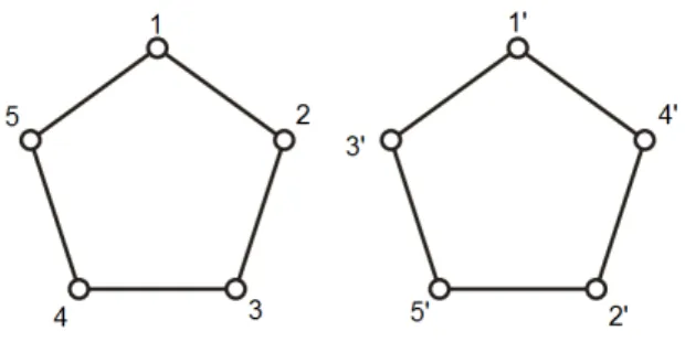
3.2 The Pentagon . . . 85
3.3 The exclusivity principle forbids sets of correlations larger than the quan-tum set . . . 86
3.4 Other graph operations . . . 90
3.4.1 Direct cosum ofG′ and G′′ . . . 90
3.4.2 Twinning, partial twinning and duplication . . . 92
3.4.3 Vertex-transitive graphs obtained fromC5. . . 93
3.5 Final Remarks. . . 94
To conclude, or not to conclude? 97 Appendix A The impossibility of non-contextual hidden variable models 99 A.1 von Neumann . . . 99
A.1.1 von Neumann’s assumptions. . . 100
A.1.2 Functionally closed sets and von Neumann’s theorem . . . 103
A.2 Gleason’s lemma . . . 105
A.2.1 Using Gleason’s Lemma to discard hidden-variable models . . . . 106
A.2.2 The “hidden” assumption of noncontextuality. . . 107
A.3 Kochen and Specker’s proof . . . 107
A.4 Other additive proofs of the Kochen-Specker theorem . . . 112
A.4.1 P-33. . . 112
A.4.2 Cabello’s proof with 18 vectors . . . 113
A.4.4 Multiplicative proofs of the Kochen-Specker theorem . . . 114
A.5 A contextual hidden-variable model . . . 117
A.6 Final Remarks. . . 118
Appendix B Non-locality 121 B.1 The EPR paradox . . . 122
B.2 Local Hidden-Variable Models . . . 124
B.3 Bell’s proof of the impossibility of hidden variables compatible with quan-tum theory . . . 125
B.4 Bell Inequalities . . . 126
B.4.1 The CHSH inequality . . . 126
B.5 Bell inequalities and convex geometry . . . 127
B.6 Final Remarks. . . 128
Appendix C What does explains the Tsirelson bound? 131 C.1 No-signaling . . . 131
C.2 Implausible consequences of superstrong non-locality . . . 133
C.3 Information Causality . . . 134
C.4 Macroscopic non-locality . . . 139
C.4.1 Macroscopically local correlations can violate Information Causality141 C.5 Quantum correlations require multipartite information principles . . . 142
C.6 Local orthogonality: the exclusivity principle for Bell scenarios . . . 144
C.7 Final Remarks . . . 145
Introduction
Foi preciso que os filósofos e outros abstractos andassem já meio perdidos na floresta das suas próprias elucubraç˜es sobre o quase e o zero, que é a maneira plebeia de dizer o ser e o nada, para que o senso comum se apresentasse prosaicamente, de papel e lápis em punho, a demonstrar por a + b + c que havia questões muito mais urgentes em que pensar.
José Saramago, As Intermitências da Morte.
Quantum theory provides a set of rules to predict probabilities of different outcomes in different experimental settings. While it predicts probabilities which match, with extreme accuracy, the data from actually performed experiments, it has some peculiar properties which deviate from how we normally think about systems which have a probabilistic description. Two of the “strange” characteristics are contextuality and nonlocality. The former tells us that we cannot think about a measurement on a quantum system as revealing a property which is independent of the set of measurements we chose to make. The latter, describes how measurements made by spatially separated observers in a multipartite quantum system can exhibit extremely strong correlations. Contextuality and nonlocality are the most striking features of quantum theory. We believe that a complete understanding of these features may be the most important step towards understanding the whole theory.
object will remain identical if they are subjected to the exactly same process. If this is not the case, we would have no reason to call them identical in the first place.
Quantum theory, on the other hand, does not provide definite outcomes for mea-surements, even if we have complete knowledge about the state of the system. If we have a large set of quantum systems, all prepared in the same state, we can apply the same measurement to all of them, obtaining a probability distribution that in general will exhibit dispersion. This means that for almost all measurements, at least two outcomes have probability larger than zero. If we apply the argument of the previous paragraph, we would conclude that the systems in this set could not be identical and hence they could not all be in the same state. Hence, the state assigned to this preparation by quantum theory cannot be everything: there are more parameters we must use in the description of these systems in order to get definite outcomes for all measurements. These unknown parameters may have different values in our set of systems, and the probabilistic behavior is due to our lack of knowledge about these “hidden variables.”
This line of thought led many physicists to believe that quantum theory might be in-complete. Hence, they conjectured the possibility of completing quantum theory, adding extra variables to the quantum description, in a way that with all this information (of quantum state plus extra variables) we would be able to predict with certainty the out-come of all measurements and in a way that when averaging over these extra variables we would get the quantum predictions. This kind of description is often called a hidden-variable model.
With some very reasonable extra assumptions on these models, we get a contradic-tion with the prediccontradic-tions of quantum theory. If the value associated by the model to a measurement is independent of what other compatible measurements are jointly per-formed, we say that the model satisfies the noncontextuality hypothesis. This demand is consistent with what we expect from classical intuition: physical quantities have pre-defined values which are only revealed by the measurement process. If these values exist prior to the measurement, how can they depend on some choice made at the moment of the measurement?
It happens that noncontextual hidden-variable models cannot reproduce quantum statistics. This result is known as the Bell-Kochen-Specker theorem. The result was first proven by Kochen and Specker, and Bell pointed out the assumption of noncontextuality, which was so natural that Kochen and Specker assumed it with no explicit discussion. A huge number of proofs can be found on the literature, much simpler then the pioneer proof. One of the most common ways to provide a simple proof of this theorem is by usingnoncontextuality inequalities. They are linear inequalities involving the probabilities of certain outcomes of the joint measurement of compatible observables that must be obeyed by any noncontextual hidden-variable model and can be violated by quantum theory with a particular choice of state and observables.
Contents
uniform relative motion. We cannot do the same for quantum theory and this is one of the most seductive scientific challenges in recent times. The starting point is assuming general probabilistic theories allowing for probability distributions that are more general than those that arise from Kolmogorov’s axioms, and even from quantum theory, and the goal is to find principles that pick out quantum theory from this landscape of possible theories. There are many ideas on how to do this, and at least three different approaches to the problem stand out.
The first one consists of reconstructing quantum theory as a purely operational probabilistic theory that follows from some sets of axioms. Imposing a small number of reasonable physical principles, it is possible to prove that the only consistent probabilistic theory is quantum [Har01, Har11, MM11, CDP11]. Although really successful, this approach does not resolve the issue completely, specially because some of the principles imposed do not sound so natural. Another drawback is that there are interesting and important quantum effects in simple systems (as opposed to composite) that cannot be addressed this way.
In the second approach, instead of trying to reconstruct quantum theory, the idea is to understand what physical principles explain the nonlocal character of quantum theory. Many different principles have been proposed, the most important being non-triviality of communication complexity, Information Causality, Macroscopic Locality and Local Orthogonality [vD12, PPK+09, NW09, OW10]. None of them is known to solve the problem completely, but many interesting results have been found so far.
The third approach consists of identifying principles that explain the set of quantum contextual correlations without restrictions imposed by a specific experimental scenario. The belief that identifying the physical principle responsible for quantum contextual-ity is better than previous approaches is based on two observations. On one hand, when focusing on quantum contextuality we are just considering a natural extension of quantum nonlocality which is free of certain restrictions (composite systems, space-like separated tests with multiple observers, entangled states) which play no role in the rules of quantum theory, although they are crucial for many important applications, specially in communication protocols (see, for example, references [Wikf, HHHH09, BBC+93] and other references therein), and played an important role in the historical debate on whether or not quantum theory is a complete theory. On the other hand, it is based on the observation that, while calculating the maximum value of quantum correlations for nonlocality scenarios is a mathematically complex problem, calculating the maxi-mum contextual value of quantum correlations for an arbitrary scenario is the solution of a semidefinite program [CSW14, Lov95]. The difficulties in characterizing quantum nonlocal correlations are due to the mathematical difficulties associated to the extra constraints resulting from enforcing a particular labeling of the events in terms of par-ties, local settings, and outcomes, rather than a fundamental difficulty related to the principles of quantum theory.
The sum of the probabilities of a set of pairwise exclusive events cannot exceed 1.
By itself, the Exclusivity principle singles out the maximum quantum value for some important Bell and noncontextuality inequalities. We can get better results if we apply the E principle to more sophisticated scenarios. This happens because this principle exhibits activation effects: a distribution satisfying this principle does not necessarily satisfy it when combined with other distributions. Activation effects can be used to prove that the Exclusivity principle singles out the set of quantum distributions for the simplest noncontextuality inequality. It is still not known if the exclusivity principle solves the problem of explaining quantum contextuality completely, but many results have been proven that support the conjecture that it does. The main purpose of this thesis is to discuss in detail the situations in which the E principle can be used to rule out distributions outside the quantum set.
In chapter 1 we start the discussion defining the generalized probability theories that are suitable for the description of states and measurements in a physical system [Bar07, BW12]. We will try to keep the assumptions as general as possible, but for the purposes of this work it is sufficient to consider a class of theories that satisfy further restrictions that do not have a physical meaning and will be made solely to simplify the description. Nonetheless, our framework is general enough to include as special cases the mathematical structure of finite dimensional quantum theory and classical probability theory with finite sample spaces.
In chapter 2 we discuss in detail the assumption of noncontextuality. We present two different approaches, both connected with graph theory: the compatibility-hypergraph approach and the exclusivity-graph approach [CSW14]. The graph-theoretical formula-tion of quantum contextuality supplies new tools to understand the differences between quantum and classical theories and also the differences between quantum theory and more general theories [Cab13b, Yan13, ATC14].
The pioneer proof of Kochen and Specker is out of the scope of this thesis, but we present it in appendix A. There the reader can find a brief discussion on the first attempts to prove the impossibility of hidden-variables models compatible with quantum theory and other interesting state-independent proofs of the Kochen-Specker theorem.
Contents
all vertex-transitive graphs with 10 vertices, except two1. These results show that the Exclusivity principle goes beyond any other proposed principle towards the objective of singling out quantum correlations. They are the main original contribution of this work. Since we made no original contribution to Bell inequalities, the concept of Bell scenarios will only be introduced in appendix B. Bell scenarios provide a natural way to enforce the noncontextuality assumption, since in these situations the experiment is designed in such a way that the choice of the different compatible observables to be measured is made in a different region of the space in a time interval that forbids any signal to be sent from one region to the other. Since no signal was sent, the choice of what is going to be measured in one part can not disturb what happens in the other, which guarantees that the model is noncontextual. In this situation, we say that the model is local and the noncontextuality assumption is usually referred to as the locality assumption.
Although nowadays we may see quantum nonlocality as a special case of quantum contextuality, historically the discussion of nonlocality in quantum theory preceded the discussion about its noncontextual character. Quantum nonlocality puzzled the famous trio Einstein, Podolsky, and Rosen, who discussed this strange property of quantum theory in their pioneer paper “Can Quantum-Mechanical description of Physical Reality Be Considered Complete?” in 1935 [EPR35]. They started one of the greatest debates in foundations of physics and philosophy of science in general, that is still fruitful nowadays. The first one to provide a proof of the impossibility of local hidden-variable models
was John Bell, in 1964 [Bel64]. He demonstrated that if the statistics of joint measure-ments on a pair of two qubits in the singlet state were given by a hidden-variable model, a linear inequality involving the corresponding probabilities should be satisfied. A simple choice a measurements leads to a violation of this inequality, and hence the model can not reproduce the quantum statistics.
Many similar inequalities were derived since Bell’s work. Because of his pioneer paper, any inequality derived under the assumption of a local hidden-variable model is called
Bell inequality. Quantum theory violates these inequalities in many situations. Besides the insight given in foundations of quantum theory, those violations are also connected to many interesting applications.
The quest for a principle that explains the set of quantum distributions in Bell scenar-ios has been very fruitful. For completeness, a brief discussion can be found in appendix C.
We will state, and sometimes prove, many results that can be found in the literature. These results will be referred to as Propositions. The original results of the author and collaborators will be referred to as Theorems. We will use a huge number of tools from many different areas of mathematics and physics. This makes a proper introduction of some subjects impractical. Typically, the necessary mathematical definitions will be given in the text, but nor its consequences, nor other previous necessary concepts will
1If the E principle explains the quantum bound for one of them, the result of Yan [Yan13] proves that
find room in the text. We list the concepts we will need, along with references where a proper discussion can be found.
1. Linear algebra: vector spaces, linear maps, matrices, basis, inner products, or-thogonal complements, tensor products; Finite dimensional Hilbert spaces. An introduction to the the subject can be found in references [HK61, Lan87];
2. Convex Geometry: we assume that the reader is familiar with the notions of convex sets, convex sums, convex cones, polytopes and H-descriptions. The reader can learn about this subjects in references [Roc97];
3. Basic probability theory: finite sample spaces,σ-algebras and measures. We give a brief introduction in section 1.4 and suggest references [SW95, GS01, Jam04] for a more complete treatment.
4. Quantum theory in finite dimension. We present the mathematical aspects in section 1.5. We recommend references [FLS65, CTDL77, Per95, NC00, Gri05, ABT11].
5. Ordered linear spaces and order unit spaces [Jam70].
6. Category theory, morphisms, opposite category, symmetric monoidal category. All these definitions can be found in reference [Mac98].
7. Sheaf theory. We define very briefly the objects we use and recommend reference [MM92] for a complete treatment.
We thank very much all who spent some of their time reading this work. Any comments, questions or suggestions are welcome.
Bárbara Amaral
[ First Chapter \
Generalized Probability Theories
In this chapter we study generalized probability theories that can be used to describe states and measurements in a physical system. We will not focus on any particular kind of system. Our intention is to discuss only the abstract mathematical structure behind the description and what the consequences are of assuming a particular type of theory. A number of requirements imposed by physical reasoning must be obeyed by all theories in this framework and for now we will try to keep the assumptions as general as possible. For the purposes of this work it is sufficient to consider a class of theories that satisfy further restrictions that do not have a physical meaning and will be made solely to simplify the description. Nonetheless, our framework is general enough to include as special cases the mathematical structure of finite dimensional quantum theory and classical probability theory with finite sample spaces, the subjects of the sections 1.5 and 1.4, respectively. In section 1.1 we define states and measurements in a physical system and in section 1.2 we discuss the mathematical description of a multipartite system. A mathematical formalization of these concepts is presented in section 1.3. We finish this chapter with general properties of the theories in section 1.6.
1.1
States and Measurements
As we said above, our purpose in this chapter is to find a suitable mathematical structure that we can apply in the description of experiments carried in a hypothetical physical system. We follow the ideas presented by Barrett in reference [Bar07].
Our first assumption is about the nature of the experiments that can be performed in this system. We assume that there are two kinds of experiments available: preparations and operations. Another important requirement is that these experiments be repeatable: every preparation and every operation can be done as many times as we want and we can use several repetitions of a given procedure to count relative frequencies. For each operation there may be several different outcomes, each occurring with a well defined probability for a given preparation. Preparations can be compared through their statistics in relation to the given operations, and these statistics define a state.
state.
Definition 2. A set of operations is called informationally complete or tomographic if the list of probabilities for the outcomes of these operations completely specifies the state of the system.
For every system there is a set of tomographic operations. In the worst case scenario, we can take the entire set of operations as a tomographic set. This is not the case in general, since only a small subset of the available operations is needed to describe the state completely. The set of tomographic operations is not unique and we will not assume it to be a minimal set, in the sense that it might be the case that removing some operations we still get a tomographic set. This set is not always finite, but we will only consider the cases in which a finite tomographic set exists.
Assumption 1. The state of the system can be completely specified by listing the probabilities of the outcomes of a finite set of tomographic operations each of them with a finite set of possible outcomes.
This restriction is not a physical requirement and it is really easy to come up with real physical systems that require an infinite set of tomographic operations or tomographic operations with an infinite number of outcomes. We are just narrowing down the kind of problems we will deal with in this work.
If we fix the set of tomographic operations{M1,M2, . . . ,Mn}, each Mi with outcomes
{1, 2, . . . ,mi}, every state can be represented by a list of probabilities:
P=
p(1|M1)
... p(m1|M1)
p(1|M2)
... p(m2|M2)
... p(1|Mn)
... p(mn|Mn)
∈Rd (1.1)
in which p(i|j) is the probability of outcome i given that the operation j was applied and d=Pn
i=1mi. Since the entries represent probabilities, we havep(i|j)≥0and
X
i
p(i|j)=1
for every tomographic operation j. Nevertheless, it will be convenient to use also sub-normalized states with
X
1.1. States and Measurements
where 0≤p≤1 and p is independent of the tomographic operation j. The value p is called the norm of the state P and will be denoted by |P|. These subnormalized states have a physical interpretation: suppose an operation j is performed in a normalized state and an outcome i is obtained with probabilityp less than one. There is a subnormalized state of the form(1.2)associated with this outcome, and each entryp(k,i|l,j)=p(i|j)· p(k|l)of this state corresponds to the probability of obtaining outcome i in operation j followed by outcomek in the tomographic operation l.
With this interpretation, the vector with all entries equal to zero, denoted by →−0, is an allowed (subnormalized) state of every system. This state can be prepared in the following way: suppose we prepare a state for which outcome i of operation M has probability zero; each entryp(k|j)of the state of the system associated to this outcome is the probability of getting i in the first operation and k in the tomographic operation j, and since outcomei is a zero probability event, all the entries of this vector are zero. Assumption 2. For each system the set of allowed normalized states is closed and convex. The complete set of statesS is the convex hull of the set of allowed normalized
states and−→0. The set S is called the state space of the system.
Definition 3. The extremal points of the state space S are called pure states. The
points that are not extremal are calledmixed states, and can be written as a convex sum of pure states. Convex sums are also called mixtures.
Definition 4. We say that a state isdispersion free if it provides definite outcomes for all measurements, that is, if for every measurement there is one outcome with probability one.
If a model admits dispersion free states, then these states are pure. The converse is not always true: some models may admit pure states that are not dispersion free. This is the case of quantum theory, as we will see in section 1.5.
When an operationM is performed, each outcomei is associated to a transformation fi of the state of the system:
P7→fi(P). (1.3)
The entry p(k|j)of fi(P) is the probability of obtaining outcome i in operation M
fol-lowed by outcomek in the tomographic operation j. Operations with only one outcome preserve normalization. If the transformation is associated with an outcome that occurs with probability p<1, then it decreases the norm of the state by a factor of p.
Definition 5. Operations with more then one outcome are called measurements. Assumption 3. We require that the transformations preserve mixtures. This means that if
P=X
i
piPi (1.4a)
then
f(P)=X
i
The physical interpretation of the vector→−0 requires that
f ³−→0´=−→0 . (1.4c)
In fact, state vector−→0 is prepared when we condition on an outcomei of a measure-ment j that happens with probability zero. Let f be associated to outcome k of some measurement l. Then the entry p(r|s) of f(−→0 ) is the probability of obtaining outcome i in the measurement j, followed by outcome k in measurement l, followed by outcome r in tomographic measurements. Since outcomei is a zero probability event in the first place, all these entries are zero and equation (1.4c)follows.
The conditions above imply that we can take f to be linear [Bar07].
Theorem 1. The transformation f associated to an operation acting on the state of a physical system can be extended to a linear operation on Rd.
Proof. Equations (1.4) imply that f(r P)=r f(P)∀ P∈S and 0≤r≤1. In fact, under
these conditions
f(r P)=f
³
r P+(1−r)→−0 ´
=r f(P)+(1−r)f(→−0 )=r f(P). (1.5) SupposeP∈S and r>1. If r P=P′∈S, then f(r P)=r f(P) since f(P)=f ¡1
rP′
¢ and by equation (1.5), f ¡1
rP′
¢
=r1f(P′). If r P∉S, we can extend f using the rule
f(r P)=r f(P). LetS
+ be the set of vectors of the form r P, P∈S, r≥0.This set is a convex cone and f(r P)=r f(P)∀ P∈S
+ and r≥0. It is also true that
f
à X
i
riPi
!
=X
i
rif(Pi), ∀ Pi∈S+, ri≥0. (1.6)
To prove this, let Pi=siPi′, si≥0, Pi′∈S and c=Pirisi. Then
f
à X
i
riPi
!
=f
Ã
cX
i
risi
c P
′
i
!
and since P
iricsiPi′∈S
f
Ã
cX
i
risi
c P
′
i
!
=c f
à X
i
risi
c P
′
i
!
=cX
i
risi
c f
¡
Pi′¢
=X
i
risif
¡
Pi′¢
=X
i
rif (Pi) .
Now we prove that equation (1.6) is also true if the coefficients ri are real. Let
Q∈S
+ such that
1.1. States and Measurements
We can rewrite the above expression as
Q+ X
ri<0
|ri|Pi=
X
ri>0 riPi
and applying f to both sides of this equation we get
f(Q)+ X
ri<0
|ri|f(Pi)=
X
ri>0
rif(Pi)
which implies
f(Q)=X
i
rif(Pi).
This proves that f is linear inS
+. IfQ belongs to the subspace spanned byS+, f(Q) can be defined uniquely by linear extension. The action on the orthogonal complement of this subspace is arbitrary and we can define it to be linear. Then f can be extended linearly to the rest of the vector space Rd.
This result implies that every transformation can be written as
f(P)=M P (1.7)
where M is a matrix acting on Rd.
An operation is associated to a set of matrices {Mi}, each Mi corresponding to
an outcome i of this operation. The subnormalized state associated to outcome i is MiP ∈S and the unnormalized probability of i is |MiP|. This means that if P is
normalized, the probability of outcome i is |MiP|.
As one should expect, not every set of matrices{Mi}corresponds to a valid operation
on the system, since some physical requirements must be satisfied.
Constraint 1. If a set of matrices{Mi}represents an operation, the following conditions
must hold
1. Positivity: 0≤|MiP|
|P| ≤1, ∀i, ∀P∈S \ {~0}; 2. Normalization: P
i|M|PiP| |=1, ∀P∈S;
3. State preservation: MiP∈S, ∀P∈S;
4. Complete state preservation: Each transformation Mi must result in allowed states
when it acts on a system that is a part of a larger multipartite system.
Assumption 4. For each system there is a setT of allowed transformations. This set
is convex and includes the transformation that takes all P to the vector→−0.
Definition 6. An operation is a set of allowed transformations{Mi}, Mi ∈T, satisfying
constraint 1.
The setT can be viewed as a set of possible outcomes for the available operations,
each outcome represented by a matrix Mi ∈T. Distinct operations may share some
outcomes, since a matrix Mi can appear in different measurements. The probability of
a given outcome does not depend on the measurement in which it appears.
Definition 7. The pair (S,T) is called a probabilistic model. A probability theory is
a collection of probabilistic models.
The same model can describe different systems. This happens because the description of a real physical system also depends on how we connect the real experiments with the mathematical objects in the model. It is also possible that the same system is described by apparently different models. For example, we could use a different set of tomographic measurements and obtain a model in a different vector space and consequently, a different set of matrices representing allowed operations. This difference is irrelevant, since the physics represented by each of them is the same.
Definition 8. Two probabilistic models (S1,T1) and (S2,T2) are equivalent if there
exist linear bijections
ξ:S1 −→ S2
ζ:T1 −→ T2
such that
|M P| = |ζ(M)ξ(P)| for every M∈T1 and everyP∈S1.1
Definition 9. If two models belong to the same equivalence class under the equivalence above, we say that they describe the same type of system.
All models describing a given type of system are equally good. Some of them might be more practical or more appropriate in a particular situation, but the choice of one instead of the others is just a mater of taste.
1.1.1
Repeatability
In the beginning of this section we mentioned that experiments must be repeatable. This means that every preparation and operation we consider can be done as many times as we want in the same conditions, what allow us to define the statistics of every sequence
1We do not assume thatS
1andS2are subsets of the same real vector space, that is, the number of
1.1. States and Measurements
of experiments. The word repeatability will be used again with a different meaning in the definition ofrepeatability of outcomes. We apologize for the inconvenient use of the same word for both concepts, but we have no better option in neither case.
Definition 10. A measurement i has repeatable outcomes if every time this measure-ment is performed and an outcome k is obtained, a subsequent measurement ofi gives outcome k with probability one.
In this chapter we still allow measurements with non-repeatable outcomes. In some cases it might be important to restrict the discussion to the case of repeatable outcomes, and we will do that further when we talk about contextuality.
1.1.2
Compatibility for outcome-repeatable measurements
One of the implications of a more general theory for computing probabilities than the usual classical probability theory is that in some cases there is not a well defined prob-ability for the results of all measurements in a given set. When this global probprob-ability distribution exists for all states, we say that the measurements are compatible. This is not new for the reader familiar with quantum theory, where non-compatibility is the rule, not the exception.
Definition 11. A set of outcome-repeatable measurements {j1, . . . ,jn} is compatible if
there is another measurement j with outcomes {1, . . . ,m} and functions f1, . . . ,fn such
that the possible outcomes of each js are fs({1, . . . ,m}) and
p¡i|js
¢
= X
k∈fs−1(i)
p¡k|j¢. (1.8)
The measurement j is called a refinement of each ji, and each ji is called a coarse
graining of j.
If the measurements {j1, . . . ,jn} are compatible, the probability of a set of outcomes
i1, . . . ,in|j1, . . . ,jn is well defined and it is equal to the probability of outcomesTkfk−1(ik)
for measurement j.
The notion of compatibility is essential in quantum theory, specially in the problems of non-contextuality we will present in chapter 2. It is connected to the idea of “mea-surements that can be performed at once”. If a set of mea“mea-surements is compatible, they can be measured jointly on the same individual system without disturbing the results of each other. In practice, to measure all of them at the same time we apply measure-ment M in definition 11 and then use functions fi to find out the outcomes of each
Mi. Compatible measurements can be made simultaneously or in any order and can be
1.2
Multipartite systems
In this section we will see how we can describe multipartite systems in general probability theories. As for the simple systems, the probability theories used for composite systems must obey some requirements that come from natural physical assumptions.
Assumption 5. For every system composed of several parties, we assume that opera-tions that act on only one of the parties are allowed. These operaopera-tions are called local operations.
Although the parties do not need to be spatially separated, this is the case most of the times we deal with multipartite systems. Thais motivates the use of the word local
for the operations acting in only one party of the system.
Assumption 6 (Local operations commute). Suppose that for each subsystem i of a multipartite system, an operation Mi is performed. Then the state of the composite
system after the sequence of operations Mi does not depend on the particular order in
which the operations were applied.
This assumption means that local operations can be regarded as performed simultane-ously on each subsystem. This implies that for each measurement the joint probabilities
p(r1, . . . ,rn|M1, . . . ,Mn)
are well defined, where ri is the outcome of measurement Mi on party i.
An important corollary of assumption 6 is that for all composite systems no-signaling holds [Bar07]. This property states that any of the parties cannot signal its choice of input to the others. Physically, this is a reasonable restriction: since there may be a large spatial separation between the parties, signaling between them would potentially require faster-then-light communication, which would violate the most fundamental principle of special relativity.
Corollary 1(No-signaling). If an operation was performed on systemi, it is not possible to get information about which operation was performed by measuring another system
j.
Proof. Suppose an operation Mi was performed on system i and afterwards we apply
operation Mj on system j. By assumption 6, the probability of getting outcome k
for measurement Mj in this sequence of operations is equal to the probability of this
outcome if Mj was performed first and then
p(k|Mi,Mj)=p(k|Mj),
which implies that p(k|Mi,Mj)does not depend on measurement Mi. This implies that
no information on Mi can be gained by any measurement in system j.
1.2. Multipartite systems
Given a system composed of n parts, it follows from the above assumption that a state of the system can be described by a vector with entries of the form
p(r1,r2, . . . ,rn|M1,M2, . . . ,Mn),
where ri is an outcome of a tomographic measurement Mi acting only on party i.
The normalized states of the composed system must satisfy X
r1,...,rn
p(r1,r2, . . . ,rn|M1,M2, . . . ,Mn)=1
but, as before, we allow subnormalized states as well. The no-signaling principle implies that, for any bipartition {S,SC} of the set {1, . . . ,n}, the marginal distribution for the parties in S obtained by summing over all outcomes of the parties i∈SC
X
ri,i∈S
p(r1,r2, . . . ,rn|M1,M2, . . . ,Mn) (1.9)
does not depend on the measurements Mi with i∈S. This means that marginal
proba-bility distributions are well defined and this allows the definition of the reduced state of a subsystemi, as the vector with entries given by2
p(ri|Mi)=
X
rj,j6=i
p(r1,r2, . . . ,rn|M1,M2, . . . ,Mn). (1.10)
Definition 12. For every state of a multipartite system described by joint probabilities of the form p(r1,r2, . . . ,rn|M1,M2, . . . ,Mn), the marginal distribution p(ri|Mi) is well
defined and is called the reduced state of partyi.
From now on, every time we refer to a multipartite system we will use only joint probabilities of local tomographic measurements to describe its state and for every sub-system we will use the same set of tomographic measurements to describe its reduced state. The connection is given by equation 1.10.
As expected, a natural constraint we will impose is that the reduced state of each subsystem is an allowed state of this subsystem.
Constraint 2. LetS be the set of allowed states for a multipartite system and Si be
the set of allowed states for a subsystem i. Let P∈S, and Pi be the reduced state of
subsystem i. We require that Pi∈Si.
The result below gives a connection between the vector spaces associated to the individual systems and the vector space associated to the composite system [Bar07]. Theorem 2. LetP be a state of a multipartite system and Pi be the reduced state of
partyi. IfP belongs to the vector spaceV and eachPi belongs to the vector spaceVi,
then
V ≡O
i
Vi.
2We can also define the reduced state of a subsetS of parties in an analogous form, using equation
Proof. We will prove the statement above for the particular case of bipartite systems. Since we only consider finite dimensional systems, the general case follows if we apply the particular case several times.
LetQi j kl12 be the vector with entry 1 for outcome i of tomographic measurement k in party 1 and outcome j for tomographic measurement l in party 2 and 0 elsewhere. Define the vectorsQ1i k andQ2j l analogously. Notice that these vectors are not necessarily allowed states of the system. Nevertheless, the vectors Q12i j kl generate V, the vectors Q1i k generateV1, the vectorsQ2j l generateV2 and
Qi j kl12 =Q1i k⊗Q2j l, which implies the desired result.
We can prove that any state of the composite system can be written as a linear combination of product states [Bar07].
Theorem 3. Any state of a n-partite system P can be written in the form
P=X
i
qiPi1⊗Pi2⊗. . .⊗Pin (1.11)
where Pij is a normalized and pure state of the party j and qi∈R.
Proof. We will once more prove the statement for n=2, since the general case follows easily from this one.
Consider a composite system consisting of parties 1and 2 in stateP∈V =V1⊗V2. By assumption 5, for each tomographic measurement l in party 2there is one operation on the composite system that corresponds to performing that measurement. Let {Mj l}
be the set of matrices representing this operation, j labeling the possible outcomes. LetPj l =Mj lP be the final state after outcome j and letP1j l be the corresponding
reduced state of system 1. Then
P=X
j,l
P1j l⊗Q2j l (1.12)
where the vectorQi j2 was defined in the proof of theorem 2.
1.2. Multipartite systems
LetU⊗W ∈V withU∈(S1)⊥. Then equation (1.12) implies that
(U⊗W)P=0.
Repeating the same argument but exchanging the parties, we conclude that for any vector of the formU⊗W with W ∈(S2)⊥ we have
(U⊗W)P=0.
This implies that P belongs to the subspace generated by U⊗W, U ∈S1 and
W ∈S2. Since each Si is generated by the states that are normalized and pure, the
result follows.
States of the formPi1⊗Pi2⊗. . .⊗Pinare calledproduct states. If a state can be written as a convex combination of product states, that is, if we can choose the coefficientsqi in
equation (1.11) such that0≤qi ≤1 and Piqi=1, it is called a separable state. States
that can not be written in this form are called entangled.
Consider a composite system and a transformation T1 acting in subsystem 1, repre-sented by the matrix M1. We know that this transformation is allowed in the composite system and that the resulting effect is linear. Hence there is a matrix M˜1 such that the
transformation on the composite system is given by
P7→P′=M˜1P.
We want to find out what the relation is between M1 and M˜1 [Bar07].
Theorem 4. Consider a multipartite system in a stateP and a local transformation M1 on subsystem 1, defined by
P17→P1′=M1P1.
The joint transformation on the composite system is given by
P7→P′=(M1⊗I⊗. . .⊗I)P. (1.13)
Proof. We will once more prove the statement for a bipartite system, since the general case follows from this one.
The probability of outcome j for tomographic measurement l in system 2 and out-comei for tomographic measurementk in system1, before transformationT1is applied, is given by entry Pi j kl=p(i,j|k,l) of vector P. After transformation T1 is applied, the
outcome j for tomographic measurementl in system 2 and outcomei for tomographic measurement k in system 1 is
Pi j kl′ =X
i′k′
Mi k1,i′kPi′j k′l=£(M1⊗I)P¤i j kl.
This implies that the action of M˜1 in S is equal to the action of M1
⊗I. Since the action of M˜1 outside S is arbitrary, we can take M˜1
=M1⊗I.
Now that we know how the action of local operations is in the description of com-posite systems, we can go back to item 4 of constraint 1 and see how this restricts the allowed transformations in each subsystem. We have stated that each local transforma-tion Mi on a subsystem i must result in a allowed state of the multipartite system as
well. This means that not only Mi has to be an allowed transformation of system i,
Mi⊗I⊗. . .⊗I has to define an allowed transformation on the composite system. This
extra requirement may reduce even further the set of allowed transformations in the individual system i.
Definition 13. A transformation T on a system 1, represented by matrix M, is well defined if
(M⊗I)P12∈S12
for all states P12∈S12, where system 2 can be any other system allowed by the theory.
Constraint 3. For each system, all transformations in T must be well defined.
System 2 can itself be a multipartite system, so the general requirement of item 4 of constraint 1 is implied by the special case of bipartite systems of definition 13 and constraint 3.
Assumption 5 together with theorem 4 imply that the allowed transformations of a composite system must include the ones given by equation (1.13).
Corollary 2. If M1is an allowed transformation on system1, then M1⊗I is an allowed transformation of a composed system consisting of system1and another arbitrary system 2.
We desire that our description include the possibility of multipartite systems with no correlation among its parties. This is quite natural: imagine that the parties of this sys-tem are thousand of kilometers apart and that none of them interacted in the past. We do not expect any correlation among the outcomes obtained in local measurement per-formed in these subsystems, and this implies that the joint probabilities are independent:
1.2. Multipartite systems
where ri is the outcome of local measurement Mi on party i.
Assumption 8. If P1 is an allowed state of system 1 and P2 is an allowed state of system2, then P1⊗P2 is an allowed state of the system composed of parties 1and 2.
The stateP1⊗P2gives independent probabilities for the bipartite system, in the form of equation (1.14). The meaning is that system 1 is in state P1, system 2 is in state
P2 and they are independent. Again, since system2 can itself be a multipartite system,
assumption 8 also implies that any vector of the form (1.14) is an allowed state of the system composed of parties1, 2, . . .n in which partyi is in state given by the probabilities p(ri|Mi).
The next assumption is another simplification without physical meaning. We will include in the set T all transformations that are mathematically well defined. There is
no physical requirement that guarantees that this is indeed the case. For a particular kind of system, it is possible that nature forbids, for some reason, some of the transformations contained in this set. As our intention is to be general, we will defineT to be the largest
set of mathematically allowed transformations.
Definition 14. A probability theory is called maximal if the set T coincides with the
set of all mathematically well defined transformations.
Assumption 9. All probability theories considered from now on are maximal.
A number of corollaries follows from this assumption. The first one is something we would like to have in our theories: the composition of two allowed transformations is an allowed transformation. Mathematically, composition of transformation represented by matrices M and N is given by the product M N. Then, if M and N are matrices associated to allowed transformations of a system, we expect thatM N is also an allowed transformation of the same system, and this is indeed the case if T satisfy assumption
9.
Corollary 3. If M,N∈T, then M N∈T.
Suppose we start with system 1 in a state P1 and we append another independent
system 2 in state P2. As we know, the state of the system composed of subsystems 1
and 2is P1⊗P2. Suppose that we apply an operation to the composite system, taking
P1⊗P2 to another stateP′, not necessarily a product state. This state gives a reduced
state P1′ that is an allowed state of system 1. This kind of procedure can be used to perform transformations on system 1 alone, and system 2is just used as an ancilla that can be discarded after the process is completed.
Corollary 4. A procedure consisting on appending an ancilla to system 1, performing
a joint operation on the composed system, and then throwing the ancilla away is a well defined transformation on system 1.
further. The reader may skip the next section with no prejudice for the understanding of the rest of the text.
1.3
A little bit of Category Theory
Previously we have defined a probabilistic model using vectors in Rd as states and matrices acting in this vector space as transformations. We can provide a more formal and general definition. The point of view we present here is a simplification of the approach of Barnum and Wilce in reference [BW12].
The first thing we need for our new definition is aordered linear space: a real vector space E equipped with a closed generating cone E+. Such a cone determines a partial ordering, invariant under translation and under positive scalar multiplication: if a,b∈E we say that a≤b iff b−a∈E+. An order unit in E is an element u∈E+ such that for every a∈E there is n∈N such that a≤nu. We use (E,u) to denote an ordered linear spaceE with an order unitu. We say that(E,u)is anorder-unit space. In this text, we will deal only with finite dimensional ordered linear spaces. In this case,E always has an order unit.
Definition 15. A state on an order-unit space E is a linear functional α∈E∗ with α(u)≤1.
Once more, our definition allows subnormalized states, with the same meaning as before. The normalized states are the ones with α(u)=1. The set of all states on E is called the state space on E and is denoted by S(E). This set is a compact and convex
set in E∗.
Definition 16. An effect on an order-unit space E is a non-zero element a∈E with a≤u and 0≤α(a)≤1, ∀ α ∈ S(E).
The set of all effects in E will be denoted by E(E). The effects in E play the role
of the elements of T. They represent possible outcomes of measurements that can be
performed on the system. Each measurement is then given by a set of effects in E. We continue following the lines of assumption 1, and this implies that we only consider measurements with a finite number of outcomes.
Definition 17. Ameasurementon an order-unit spaceE is a finite setO={a1,a2, . . . ,an}
of effects ai with
a1+a2+. . .+an=u.
If α is a normalized state, the probability of obtaining outcome ai in measurement
O is α(ai). Different measurements can share an outcome ai, and the probability of
obtaining this outcome is independent of the measurement in which it appears.
Once a measurement is performed and a given outcome is obtained, the state of the system will change, and hence every effect is related to a transformation on S(E), that
1.3. A little bit of Category Theory
Definition 18. A probabilistic model is given by an order-unit space E, which deter-mines the state-spaceS(E) and the set of effects E(E).
Here we assume thatS(E)contains all mathematically well defined states and E(E)
contains all mathematically well defined effects. More restrictive models can be consid-ered, but we will not deal with them in this text.
Multipartite systems can be represented using composition of models. The compo-sition will be another model, together with a way of connecting states and effects in the single system with some particular states and effects of the composite system.
Let E and F be two order-unit spaces, representing systems 1 and 2 respectively. The composite system whose parts are 1 and 2is represented in a order-unit space E F, together with a positive linear mapping
E×F −→ E F
(a,b) 7→ ab. (1.15)
This mapping gives the connection between states and effects of E and F and E F we mentioned above. Its positivity implies that if a is an effect on E and b is an effect on F, ab is an effect onE F. A number of other requirements must be satisfied by this map and also by the states in E F∗. All assumptions made in section 1.2 will hold for states and effects in E F as well. Since we already provided a detailed discussion there, we will not repeat it here. For a different and more mathematical point of view and also for a discussion of the conditions we must impose in the map of equation (1.15), see reference [BW12].
1.3.1 Processes and Categories
A theory aiming to describe physical systems has to provide rules that must be obeyed when a system changes. We already discussed these rules when this change does not alter the type of system we are dealing with, but it might be the case that it does alter the type of the system we are trying to describe. We have then to define what are the valid mappings between different types of systems. These mappings are called processes. Definition 19. Given two order-unit spaces (E,u) and (F,v), a process is a positive linear mapping
φ:E∗−→F∗ with φ(α) (v)≤α(u)for all states α in (E,u).
Definition 20. A process φ:E∗→F∗ is well defined if
φ⊗I: (EG)∗−→(F G)∗
also takes states on EG∗ to states on (F G)∗, for every order-unit spaceG, where (EG)∗ is the state space of the system composed of parties E andG,F G∗ is the state space of the system composed of partiesF andG andφ⊗I is the extension ofφ to the composite systemEG (which is defined as applying φto systemE and doing nothing in systemG). Process must take allowed states of the system to allowed states also when the system under consideration is a part of a multipartite system. That is why we require that all processes are well defined.
We also assume that convex combinations and composites of processes are also processes, for the obvious reasons. For every pair of order-unit spacesE andF there is a null process that takes every states α∈E∗ to the zero vector in F∗. The interpretation of this state is the same as before, and it can be prepared conditioning in a outcome of a measurement that happens with probability zero.
We postulate the existence of a canonical trivial system I with a single operation, and hence with no measurement. For this system, E=E∗=R. We do not have many options in this case, since the only normalized state is 1, which gives probability one for the only possible effect.
Given an order-unit spaceE, there are two kinds of natural processes involvingE and the trivial systemI. The first one is a mathematical representation of the experiment that preparates a state. For every normalized stateα∈E∗ we define the processφα:R−→E∗
of preparation of α given by
17→α.
The second kind of process is a mathematical representation of obtaining the outcome related to an effect in a measurement. For every effect a we define the process ψa :
E∗−→R of registration of the outcome a, taking α to α(a). Definition 21. A probabilistic category is a category C such that
1. Every object inC is a probabilistic model, including the trivial;
2. The set of morphisms between two objects inC is the set of well defined processes
between the corresponding models.
The set of effects on a order-unit space E can be identified with a subset ofC(E,I)
by the injection
a7−→ψa:E∗→R
that takes each effect a∈E to the corresponding registration process ψa, and the set of
all states on E can be identified with a subset of C(I,E)by the injection