AnaWEGE: a weather generator based on analogues of atmospheric circulation

(1)

GMDD

6, 4745–4774, 2013

Circulation analogue weather generator

P. Yiou

Title Page Abstract Introduction Conclusions References

Tables Figures

◭ ◮

Back Close

Full Screen / Esc

Printer-friendly Version Interactive Discussion

Discussion

P

a

per

|

D

iscussion

P

a

per

|

Discussion

P

a

per

|

Discuss

ion

P

a

per

|

Geosci. Model Dev. Discuss., 6, 4745–4774, 2013 www.geosci-model-dev-discuss.net/6/4745/2013/ doi:10.5194/gmdd-6-4745-2013

Geoscientiic Geoscientiic

Geoscientiic

Open Access

Geoscientiic

Model Development

Discussions

This discussion paper is/has been under review for the journal Geoscientific Model Development (GMD). Please refer to the corresponding final paper in GMD if available.

AnaWEGE: a weather generator based on

analogues of atmospheric circulation

P. Yiou

Laboratoire des Sciences du Climat et de l’Environnement, UMR8212 CEA-CNRS-UVSQ, CE Saclay, l’Orme des Merisiers, 91191 Gif-sur-Yvette cedex, France

Received: 1 August 2013 – Accepted: 2 September 2013 – Published: 13 September 2013 Correspondence to: P. Yiou (pascal.yiou at lsce.ipsl.fr)

(2)

GMDD

6, 4745–4774, 2013

P. Yiou

Tables Figures

◭ ◮

Back Close

Full Screen / Esc

Discussion

P

a

per

|

D

iscussion

P

a

per

|

Discussion

P

a

per

|

Discuss

ion

P

a

per

|

Abstract

This paper presents a stochastic weather generator based on analogues of circulation (AnaWEGE). Analogues of circulation have been a promising paradigm to analyse cli-mate variability and its extremes. The weather generator uses precomputed analogues of sea-level pressure over the North Atlantic. The stochastic rules of the generator con-5

strain the continuity in time of the simulations. The generator then simulates spatially coherent time series of a climate variable, drawn from meteorological observations. The weather generator is tested for European temperatures, and for winter and sum-mer seasons. The biases in temperature quantiles and autocorrelation are rather small compared to observed variability. The ability of simulating extremely hot summers and 10

cold winters is also assessed.

1 Introduction

Weather generators are tools to generate random time series of climate variables (gen-erally precipitation, temperature or wind speed) with realistic statistics. Such statistics can be the mean, variance or quantiles of the variables. More sophisticated statis-15

tical quantities can be evaluated (e.g., persistence, power spectra, skewness, etc.), depending on the application of the weather generator. Their realism is tested on me-teorological observations. Their use is mainly to simulate long series at local spatial scales that are not accessible to general circulation models (GCMs) or even regional climate models (RCMs). The probability distributions of relevant climate variables can 20

hence be estimated from those weather generator simulations.

(3)

GMDD

6, 4745–4774, 2013

P. Yiou

Tables Figures

◭ ◮

Back Close

Full Screen / Esc

Discussion

P

a

per

|

D

iscussion

P

a

per

|

Discussion

P

a

per

|

Discuss

ion

P

a

per

|

a few minutes. This ease of use has been an incentive for the development of such applications.

One of the limitation of many random weather generators is their lack of spatial co-herence, unless it is imposed on the marginal distributions of a variable at two locations

or more (Naveau et al., 2009). Such a spatial constraint is technically difficult to impose,

5

even with copulas (Schölzel and Friederichs, 2008), because of the infinity of possible choices of parameters. Methodologies considering spatial coherence have been tested for precipitation in the USA (Wilks, 1999; Schoof and Robeson, 2003) .

This paper presents a random weather generator (AnaWEGE) based on circulation analogues (Vautard and Yiou, 2009; Yiou et al., 2012). This weather generator pre-10

serves spatial constraints by construction and can be used to generate time series of climate variables such as temperature, precipitation or wind speed, distributed over a continent. The paper first presents the method of analogues of circulation. Two rules are proposed for a stochastic weather generator based on analogues of circulation. The first one is a perturbation of an observed sequence of climate variables. The second 15

one allows one to explore several likely sequences of a climate variable. This weather generator is tested for temperature observations over Europe, with a focus on time au-tocorrelation, and quantile properties. The ability of the weather generator to simulate hot summers and cold winters is also tested. The motivation stems from an application to the energy sector, because peaks of energy consumption occur during cold winters 20

(for heating) and hot summers (for air conditionning).

2 Analogues of circulation

The preliminary step of the weather generator is to compute analogues of circulation. This computation is done once (before using the weather generator), and the resulting analogues are used to generate weather time series. Here, the terminology of Yiou 25

(4)

GMDD

6, 4745–4774, 2013

P. Yiou

Tables Figures

◭ ◮

Back Close

Full Screen / Esc

Discussion

P

a

per

|

D

iscussion

P

a

per

|

Discussion

P

a

per

|

Discuss

ion

P

a

per

|

from the National Centers for Environmental Prediction (NCEP) reanalysis data (Kalnay et al., 1996) for daily SLP between 1st Jan. 1948 and 31st Dec. 2012. The SLP data

have a horizontal resolution of 2.5×2.5◦. We focus on the North Atlantic region (80◦W–

30◦E; 30◦N–70◦N). Of course other reanalysis data sets or climate model simulations

could be substituted to the NCEP reanalysis, for instance CMIP5 simulations (Taylor 5

et al., 2012).

Each dayj between 1 January 1948 and 31 December 2012 can be written:

j=y104+m102+d, (1)

wherey is the year (between 1948 and 2012),mis the month (between 1 and 12) and

d is the day (between 1 and 31). In the sequel, days of the year are encoded in this

10

manner. By convention, thecalendar day ofj is:

κ(j)=m102+d. (2)

For each “target” dayj, the setS_j of daysj′=y′104+m′102+d′is determined, where

y′6=y, and the calendar distance |j−j′| between j and j′ is less than 30 days. The

calendar distance is the number of days that separateκ(j) andκ(j′). The setSj is:

15

S_j={j′=y′104+m′102+d′,y′6=y,|j−j′| ≤30}. (3)

The analogues are computed by minimizing the root mean square (RMS) distance

between SLP[j] and SLP[j′] overS_j:

D(j,j′)=

" X

x

(SLP[x,j]−SLP[x,j′])2

#1/2

, (4)

wherex is the spatial dimension. Here the firstK =20 analogues of the target SLP of

20

(5)

GMDD

6, 4745–4774, 2013

P. Yiou

Tables Figures

◭ ◮

Back Close

Full Screen / Esc

Discussion

P

a

per

|

D

iscussion

P

a

per

|

Discussion

P

a

per

|

Discuss

ion

P

a

per

|

The choice of the RMS as a distance to minimize is debatable. Other distances can be chosen (e.g., Mahalanobis or “taxicab”). The Mahalanobis (1936) distance is potentially interesting because it normalizes the data by their spatial covariance structure. But it is a computational burden that makes it almost ten times slower than RMS, due to repeated products of large matrices.

5

For each day j∈ [1 January 1948, 31 December 2012], K=20 analogues of SLP

are obtained, with days J_jk (k∈[1,K]) in years different than those of j. For all

ana-logues, the spatial rank correlation between SLP[j] and SLP[J_jk] is computed. This

score is used to provide an objective degree of similarity between the target SLP and

its analogues: correlation values lie between−1 and 1 andpvalues can be obtained for

10

statistical significance. The (Spearman) rank correlation measures the pattern similar-ity, rather than the average field proximity captured by the distance, although correlation

is not adistancein the mathematical sense.

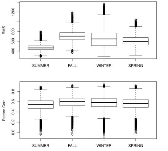
The 20 first analogues are computed for all days of SLP for the NCEP reanalysis. The distribution of RMS and correlation values are indicated in Fig. 1. They are com-15

puted for the four seasons (winter, spring, summer and fall). The RMS values exhibit a seasonal cycle, with higher values in the Fall and Winter. This is due to a higher variance of SLP in the cold seasons than in the warm seasons. The correlation values also yield a seasonal cycle, albeit with a much smaller amplitude. High correlations are found in the winter, and lower correlations appear in the summer. This is explained by 20

less contrasted spatial patterns in the summer than in the winter, so that the average RMS can have a small value, but the spatial patterns can be shifted for the analogues. This was explained by Yiou et al. (2012).

In the following, for each dayj, the setJ ofK =20 analogues days is written:

J={jˆk,k∈[1,K]}, (5)

25

with (decreasing) RMS values:

(6)

GMDD

6, 4745–4774, 2013

P. Yiou

Tables Figures

◭ ◮

Back Close

Full Screen / Esc

Discussion

P

a

per

|

D

iscussion

P

a

per

|

Discussion

P

a

per

|

Discuss

ion

P

a

per

|

and spatial correlation values:

C={ck,k∈[1,K]}. (7)

The distribution of the maximum, median and minimum correlations of the 20 ana-logues is shown in Fig. 2 (upper panel). This shows that the highest correlation among

the 20 analogues exceedsr =0.6 in 75 % of cases, and the minimum correlation is

5

significantly positive in 75 % of cases.

For each day, the analogues with the maximum, median and minimum correlations are determined. Their ranking according to RMS value is shown in Fig. 2 (lower panel). This shows that the analogues with high correlation, median or low correlations roughly yield low, medium and high RMS values, although correlations and RMS values are not 10

correlated in general.

In practice, the computation of circulation analogues is done once. The computation is done in R. It can be accelerated by parallelization, because each analogue com-putation is done independantly from the others. It produces a multi-column text file. Each line represents a day between 1 January 1948 and 31 December 2012. The first 15

column is the date of the target day. The 20 following columns are for the dates of ana-logues. The 20 following columns are for the RMS values. The last 20 columns are for the Spearman spatial correlation values. It serves as input to the weather generator.

3 Generating random sequences from SLP analogues

The goal of the weather generator is to produce a random sequence of dates (between 20

1 January 1948 and 31 December 2012) with a temporal coherence. A random

re-sampling of the calendar would not be sufficient because time continuity of the SLP

field would be lost. Thus two methodologies are presented for creating random sam-ples of dates from analogues in order to preserve time continuity of SLP. The rationale of those methodologies stems from dynamical system theory and ensemble weather 25

(7)

GMDD

6, 4745–4774, 2013

P. Yiou

Tables Figures

◭ ◮

Back Close

Full Screen / Esc

Discussion

P

a

per

|

D

iscussion

P

a

per

|

Discussion

P

a

per

|

Discuss

ion

P

a

per

|

SLP and shadows it from a random selection of analogues. The second methodology (called “dynamic”) computes a new trajectory from a selected initial condition, with a constraint of staying on the underlying attractor.

3.1 Static weather generator

The weather generator selects random years (between 1948 and 2012). The goal is 5

to generate ensembles of seasons of typically 90 days. The season to be simulated is

writtenS (e.g. winter, spring, summer or fall). For each selected random year (y), the

datesjSin the seasonSare considered. Each dayjS is replaced by a random sample

of (j_S, ˆj1,. . ., ˆjK) with probabilities:

p₌(p0,p1,. . .,pK). (8)

10

The value of p0=βα1 gives a probability of not changing jS. The probabilities

{p1,. . .,pK}are chosen to be proportional to the spatial correlation between analogue

and observed SLPC:

pk=β(1+ck)/2. (9)

βis a normalization factor so that the sum of probabilities equals 1:

15

K

X

k=0

pk=β α1+ K

X

k=1

(ck+1)/2

!

=1. (10)

This procedure randomly transforms observed trajectories with weights on “resembling” analogues: each day is perturbed independently of other days on the reference

trajec-tory. It is calledstatic because the transformed trajectory does not have the possibility

of jumping to a very different trajectory of the underlying climate attractor. This method

20

(8)

GMDD

6, 4745–4774, 2013

P. Yiou

Tables Figures

◭ ◮

Back Close

Full Screen / Esc

Discussion

P

a

per

|

D

iscussion

P

a

per

|

Discussion

P

a

per

|

Discuss

ion

P

a

per

|

3.2 Dynamic weather generator

For each day (or initial condition), the next step of the trajectory is estimated, knowing that there is an uncertainty in the observation of the initial condition. Hence, the weather generator looks at the nearest neighbors (i.e. the analogues) of the initial condition and examine the trajectories emerging from those nearest neighbor initial conditions. 5

The proposed methodology assigns probability distributions to the nearest neighbors in order to compute random (but likely) trajectories of the system.

The generator is initialized by a random day j0=10

4

y0+10 2

m0+d0. Let the day

coming afterj0be ˆj. This day hasK =20 analogues:

J={jˆk,k∈[1,K]}, (11)

10

with spatial correlation values:

C={ck,k∈[1,K]}. (12)

The weather generator choses a random “next day” forj0 among ˆj and its analogues

J. Hence a probability vector is assigned:

p₌(p0,p1,. . .,pK) (13)

15

to those potential “next days”. The most likely candidate should certainly be ˆj, so that

p0 is proportional to a high valueα1. The value of α1 controls the persistence of the

generator: ifα₁is too high, the generated sequence will mostly be consecutive days in a

deterministic fashion. The probabilities{p1,. . .,pK}are chosen to be proportional to the

spatial correlation and the calendar distance between ˆjkandj0. This condition ensures

20

an average seasonal cycle in the simulated series of dates. Hence, the probabilities

{p1,. . .,pK}are taken as:

pk=β(ck+1) exp−α2|jˆk−j0|

(9)

GMDD

6, 4745–4774, 2013

P. Yiou

Tables Figures

◭ ◮

Back Close

Full Screen / Esc

Discussion

P

a

per

|

D

iscussion

P

a

per

|

Discussion

P

a

per

|

Discuss

ion

P

a

per

|

Theα2parameter controls the weight given to the calendar proximity of the analogues.

If α is large, only analogues that have calendar dates close to the one of j0 will be

chosen. Theβparameter is determined so that the sum of probabilities equals 1:

K

X

k=0

pk=β α1+ K

X

k=1

(ck+1) exp−α2|jˆk−j0|

!

=1. (15)

From the vector of probabilitiesp, one “next” datej1forj0is sampled. The operation

5

is then repeated for the desired number of iterations.

The free parameters of the weather generator areα1(persistence) andα2

(season-ality). By default, the values are α1=0.5 and α2=4. By construction, a positive α2

ensures that a seasonal cycle in the simulations if one is interested in simulating long time series (and not just a large ensemble of seasons). This parameter also constrains 10

the dynamic weather generator to flow “forward” in time, because analogue dates oc-curring far away from the desired calendar date have a very low probability of being drawn.

This operation can be repeated for an arbitrary number of time steps. The outcome

of this simulation is a sequencejof dates of analogues:

15

j₌{j0,. . .,jN}. (16)

If one is interested in simulating weather conditions for a given season, one can

ini-tializej₀ with a random year and a calendar day starting the season (e.g. 21 March,

June, September or December) and let the weather generator run for 90 days and an arbitrary number of seasons.

20

This type of Monte Carlo simulation (simulating a large number of seasons) can be

done in parallel, in order to increase the efficiency of the computation. The weather

generator code has been tested on a computing server with 2 to 8 CPUs.

(10)

GMDD

6, 4745–4774, 2013

P. Yiou

Tables Figures

◭ ◮

Back Close

Full Screen / Esc

Discussion

P

a

per

|

D

iscussion

P

a

per

|

Discussion

P

a

per

|

Discuss

ion

P

a

per

|

weather generator is initialized with SLP conditions at the beginning of the summer of 2003, it is possible to assess the probability of observing a major European heatwave by repeating simulations. The weather generator hence works like a seasonal climate prediction, with a very large ensemble. The provided code in R is not configured to do an actual seasonal prediction.

5

4 Simulation of European temperatures

In this section we are interested in simulating mean daily temperature anomaly varia-tions at a given location, or a set of locavaria-tions in western Europe. The goal is to combine existing observations and the sequence of dates produces by the random analogues.

4.1 Composites of temperatures from analogues 10

We want simulate random temperature anomalies T with respect to a seasonal

cy-cle, at a given location that are coherent with the large scale information given by the

sequencej₌(j0,. . .,jN) obtained in Sect. 3. It is assumed that there are daily

obser-vationsT_j during the reanalysis period (j∈[1 January 1948, 31 December 2012]). The

simulation of temperature variations simply considers the set of temperatures ˆT:

15

ˆ T=(T_j

0,. . .,TjN). (17)

Therefore, composite temperatures for a random selection of analogues are deter-mined.

The advantage of this approach appears when one wants to simulate temperature at several stations. By construction, the local temperature simulations are consistent with 20

large scale SLP on daily time scale. This implies that for each day, the simulated tem-peratures at two or more locations are coherent with each other. This can be achieved

with copula that model the multivariate dependence of several time series (Schölzel

(11)

GMDD

6, 4745–4774, 2013

P. Yiou

Tables Figures

◭ ◮

Back Close

Full Screen / Esc

Discussion

P

a

per

|

D

iscussion

P

a

per

|

Discussion

P

a

per

|

Discuss

ion

P

a

per

|

needs to be re-evaluated if one set of observations is added or substracted. Here, the spatial dependence structure is provided by the SLP analogues.

With this simple first procedure, the values of ˆT are drawn from the values of the

observations. What changes is the sequence of values. For anN=90 day season, the

number of possibilities for a simulated trajectory is of the order ofKN>10117ifK =20

5

analogues are used. If persistence constraints of a few days are imposed, with large

values ofα₁, this still leaves a large number of possibilities.

In summary, the weather generator for temperature proceeds in four steps:

1. Read SLP analogues and Pareto parameters for temperature at selected loca-tions.

10

2. Simulation of random dates from SLP analogues (static or dynamic).

3. Computation of temperatures for simulated dates for selected locations.

Time series of climate variables can be saved in various formats. By default, the native R binary format is used for output.

4.2 Data 15

In principle, the weather generator can simulate temperatures for any location, provided that it yields observations. We opted to focus on European temperatures. The Euro-pean Climate Assessment and Data (ECA&D) dataset provides a regularly updated set of observations done by meteorological services over Europe (Klein-Tank et al., 2002). Time series are provided on a daily timescale. The data have been homoge-20

nized and quality checks were performed by the data providers. Data and metadata available at http://www.ecad.eu.

A subset of 291 series from the 1872 average temperature time series of ECA&D (TG) was selected. Time series starting before 1948 and ending after 2012 (hence covering the NCEP reanalysis period) were chosen. Stations for which more than 10 % 25

(12)

GMDD

6, 4745–4774, 2013

P. Yiou

Tables Figures

◭ ◮

Back Close

Full Screen / Esc

Discussion

P

a

per

|

D

iscussion

P

a

per

|

Discussion

P

a

per

|

Discuss

ion

P

a

per

|

with a high density of stations in Germany. For each time series, a seasonal cycle was computed by averaging over calendar days between 1971 and 2000. The seasonal cycle was then smoothed by a spline (smooth.spline) with 9 degrees of freedom. The seasonal cycle was removed to daily temperature values in order to obtain temperature anomalies.

5

5 Metrics and bias estimates

Here the weather generator for summer and winter temperatures in Europe is tested. The weather generator is run for 100 winters and summers of 90 days. Two sets of experiments were performed for each season. The first one set is initialized with a random year between 1948 and 2011. Such an experiment tests the climatological fea-10

tures of the weather generator. The second type of experiment initializes the weather generator from years that have experienced extreme temperatures, with hot summers and cold winters. The prototype year for hot summer is 2003 (Schaer et al., 2004). The prototype years for cold winters is 2009. Such experiments test the ability to simulate extreme temperatures (Cattiaux et al., 2010).

15

The average daily mean temperature (TG) anomaly was simulated for all 291 sta-tions. The 5th, 25th, 50th, 75th and 95th quantiles of temperature were computed for the observed time series (between 1948 and 2011) and the simulated time series. The comparison of quantiles allows one to verify the probability distribution induced by the weather generator.

20

The autocorrelation function was also computed for the observed and simulated time series of temperature for each 3 month season. At lag 0, the autocorrelation function

is 1 (by construction). It tends to 0 when the lag tends to infinity. The first lag timeτ

for which the autocorrelation is no longer significantly positive is considered. This lag

τ provides a measure of the persistence of temperature variations. The value ofτ is

25

computed for each simulated season. It is then possible to compare the quantiles ofτ

(13)

GMDD

6, 4745–4774, 2013

P. Yiou

Tables Figures

◭ ◮

Back Close

Full Screen / Esc

Discussion

P

a

per

|

D

iscussion

P

a

per

|

Discussion

P

a

per

|

Discuss

ion

P

a

per

|

5.1 Summer temperatures

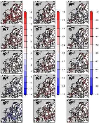
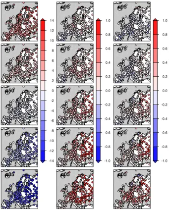
In those sets of experiments, the summers were initiated on the 21st of June. The five quantiles (5, 25, median, 75 and 95) of temperature anomalies from the ECA&D database are shown in Fig. 3 (left column), for reference. 90 % of temperature anomaly

values range between−6 and 10◦C. For each quantile, the differences between

obser-5

vations and simulations are shown in Fig. 3 (central and right column) for the static and dynamic weather generators.

The static weather generator has a generally slight warm bias (<0.6◦C). The bias is

less than 0.2◦C in France or Great Britain.

The bias for the dynamic weather generator is slightly positive for the lower quan-10

tiles (<0.4◦C). It yields small negative values (<0.2◦C), especially in Germany, for the

upper quantiles.

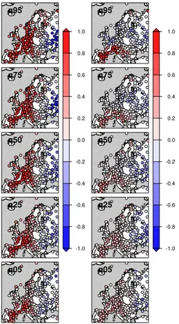
The extreme summer conditions were simulated with initializations on 21st of June

2003. The quantile differences are shown in Fig. 5. The static weather generator, by

construction, simulates high temperature differences for all quantiles, especially for

15

France. This is to be expected because such simulation only alters each day of summer 2003 with analogue SLP. During the summer of 2003, the weather patterns were mostly anticyclonic, and caused the major observed heatwave in Western Europe (Cassou et al., 2005).

The dynamic simulations yield more moderate temperature positive anomalies in 20

Western Europe, although the anomalies have higher values for the upper quantiles. This means that not all synoptic conditions resembling those at the beginning of the summer 2003 lead to a major heatwave. This was the case, for instance, for the year 2005 in Europe, which had similar weather patterns as 2003 at the end of June, but did not reach a heatwave at the middle of the summer. This result however suggests 25

(14)

GMDD

6, 4745–4774, 2013

P. Yiou

Tables Figures

◭ ◮

Back Close

Full Screen / Esc

Discussion

P

a

per

|

D

iscussion

P

a

per

|

Discussion

P

a

per

|

Discuss

ion

P

a

per

|

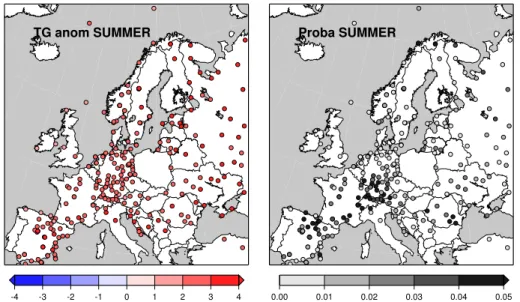
From the set of 100 dynamic experiments starting on 21 June 2003, the stationwise probability of simulating a summer with an average temperature exceeding the 90th quantile of observed mean temperature between June and August over Europe since 1948 is computed (this corresponds to the 6th hottest summer). It is found that this probability lies around 1 % in Europe. This probability exceeds 3 % in Spain, Eastern 5

France, Switzerland and Germany (Fig. 6). This means that, although the simulated temperatures are on average warmer than usual, the probability of obtaining an ex-tremely warm summer is small. This test is very conservative, because the radius of European heatwaves is less than 1000 km, and the criterion used here considered the whole of Europe.

10

5.2 Winter temperatures

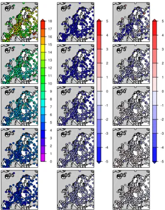
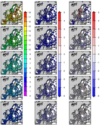
In those sets of experiments, the summers were initiated on the 21st of December. The five quantiles (5, 25, median, 75 and 95) of temperature anomalies from the ECA&D database are shown in Fig. 7 (left column), for reference. 90 % of temperature anomaly

values range between−14 and 10◦C. For each quantile, the differences between

ob-15

servations and simulations are shown in Fig. 7 (central and right column) for the static and dynamic weather generators.

The static weather generator has a generally warm bias (<1◦C) (Fig. 7, central

col-umn). The bias is less than 0.6◦C in France or Great Britain. This warm bias is larger

for the extremely low quantiles (5th quantile), especially in central Europe. The bias 20

over Western Europe for quantiles above the 25th are generally smaller than 0.2◦C.

The dynamic weather generator also yields a positive bias for temperature under

the 25th quantile (Fig. 7, right column). This bias is lower than 0.2◦C above the 25th

quantile.

The extreme winter conditions were simulated with initializations on 21st of Decem-25

ber 2009. The quantile differences are shown in Fig. 9. The static weather generator, by

construction, simulates highly negative temperature di_fferences for all quantiles,

(15)

GMDD

6, 4745–4774, 2013

P. Yiou

Tables Figures

◭ ◮

Back Close

Full Screen / Esc

Discussion

P

a

per

|

D

iscussion

P

a

per

|

Discussion

P

a

per

|

Discuss

ion

P

a

per

|

of winter 2009/2010 with analogue SLP. During the winter of 2009/2010, the weather patterns were locked to a negative phase of the North Atlantic Oscillation, and caused the major observed cold spell in Western Europe (Cattiaux et al., 2010; Cohen et al., 2010).

The dynamic simulations yield more moderate temperature negative anomalies in 5

Western Europe (Fig. 9, right column). The temperature differences are more

nega-tive for Northern Europe (incl. Germany and Great Britain). When they are posinega-tive

(e.g. in France for the lower quantiles), the quantile differences are smaller than for the

climatological simulations in (Fig. 7, right column). This implies that the simulated tem-peratures starting in December 2009 are colder than the ones obtained from a random 10

year. This also suggests that a winter that starts like the 21 December 2009 is likeky to be colder than usual.

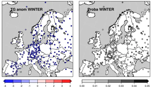
From the set of 100 dynamic experiments starting on 21 December 2009, the sta-tionwise probability of simulating a winter with an average temperature below the 10th quantile of observed mean temperature between December and February over Europe 15

since 1948 is computed (this corresponds to the 6th coldest winter). It is found that this probability lies around 1 % in Europe. This probability lies between 1 and 3 % in North-ern Spain, France, Switzerland and Germany (Fig. 10). This means that, although the simulated temperatures are on average colder than usual, the probability of obtaining an extremely cold winter is small.

20

6 Conclusions and perspectives

A weather generator based on analogues of atmospheric circulation is presented in this paper. The main feature of this weather generator (AnaWEGE) is that it can simulate meteorological variables at a set of locations (in Europe) and achieve a natural spatial coherence due to physical relationships between large scale and small scale variability. 25

(16)

GMDD

6, 4745–4774, 2013

P. Yiou

Tables Figures

◭ ◮

Back Close

Full Screen / Esc

Discussion

P

a

per

|

D

iscussion

P

a

per

|

Discussion

P

a

per

|

Discuss

ion

P

a

per

|

The constraints of the dynamical generator (theα1 andα2parameters) ensure that a

seasonal cycle is obtained if a long continuous time series is desired.

AnaWEGE yields static and dynamic modes, and can serve two different purposes:

– the generation of ensembles of random perturbations of observed climate

trajec-tories. This is useful for generating large catalogues of events (e.g. heatwaves or 5

coldspells). In terms of regional climate simulation, this corresponds to anudging

procedure with observed large scale conditions.

– the generation of ensembles of trajectories from given initial conditions. This is

useful for assessing probability distributions of events, for instance by chosing ini-tial conditions preceding the events. This feature is similar to a numerical weather 10

forecast, although it uses an already computed reanalysis dataset as a basis (or could use any model simulation). Such an option is a very cheap alternative (al-beit with no physical constraint) to real atmospheric model simulations, although large ensembles can be achieved without the use of a supercomputer.

AnaWEGE was tested on European surface temperatures, from the ECA&D data 15

(Klein-Tank et al., 2002), for which a dedicated computation of daily anomalies is pro-vided. The rationale for focusing on temperature was to provide a tool to estimate back-ground temperature extremes (especially in winter and summer), for European energy providers. The weather generator can be extended to simulate other climate variables (such as precipitation or wind speed), provided that time series of observations on 20

the same time span as the set of circulation analogues is available. The analogues of circulation yield good skill for European precipitation (Vautard and Yiou, 2009) and geopotential height (Yiou et al., 2012).

This weather generator can serve as a basis for more sophisticated weather gen-erators, which can add layers of randomness over the values that it generates. For 25

(17)

exam-GMDD

6, 4745–4774, 2013

P. Yiou

Tables Figures

◭ ◮

Back Close

Full Screen / Esc

Discussion

P

a

per

|

D

iscussion

P

a

per

|

Discussion

P

a

per

|

Discuss

ion

P

a

per

|

ple, values of a climate variable exceeding a chosen threshold can be replaced by a simulation of a Pareto distribution (e.g. Vrac and Naveau, 2008; Bonazzi et al., 2012).

An underlying hypothesis of the weather generator is a stationary climate, in order to simulate stationary time series, which is certainly not true for observed European

temperature, although the temperature trend (≈0.5◦C in 50 yr) is lower than the

intra-5

seasonal and interannual variability.

Weather generators have been used to downscale climate variables in simulations of future climates (Carter, 1996; Iizumi et al., 2012). The weather generator presented here can be used in such a configuration once circulation analogues are computed for scenario simulations (Taylor et al., 2012), provided that their SLP output is available on 10

daily time increments.

The computer performance of AnaWEGE might not be as high as already existing ones (Mavromatis and Hansen, 2001; Huth et al., 2001; Hansen et al., 2006; Semenov

and Barrow, 1997; Flecher et al., 2010). It takes≈2 min to make 100 simulations of

an 90 day season on a computer with two processors, with the parallel option. A rudi-15

mentary user manual is available with the programmes. AnaWEGE requires packages (snowfall for parallel computing and evd for optional Pareto distributions) that are avail-able on the R web site. The source code, input data files and a rudimentary user manual of version 1.0 can be downloaded at: http://www-lscedods.cea.fr/AnaWEGE/

It is designed for scientific research (no gui interface) and the parameters can be 20

changed easily. The season_sim_v1.R file is a wrapper to initialize and run the weather generator. Computer system path parameters need to be adapted for each user. The data files (analogues and mean daily temperature anomalies over Europe) are provided for an immediate use of the weather generator. The weather generator is hence a very versatile tool, especially if one generates files of analogues from other reanalyses or 25

(18)

GMDD

6, 4745–4774, 2013

P. Yiou

Tables Figures

◭ ◮

Back Close

Full Screen / Esc

Discussion

P

a

per

|

D

iscussion

P

a

per

|

Discussion

P

a

per

|

Discuss

ion

P

a

per

|

Acknowledgements. This work was supported by the Climate KIC project E3P. The codes are written in R language.

The publication of this article is financed by CNRS-INSU.

References 5

Bonazzi, A., Cusack, S., Mitas, C., and Jewson, S.: The spatial structure of European wind storms as characterized by bivariate extreme-value copulas, Nat. Hazards Earth Syst. Sci., 12, 1769–1782, doi:10.5194/nhess-12-1769-2012, 2012. 4754, 4761

Carter, T. R.: Developing scenarios of atmosphere, weather and climate for northern regions, Agr. Food Sci. Finland, 5, 235–249, 1996. 4761

10

Cassou, C., Terray, L., and Phillips, A. S.: Tropical Atlantic influence on European heat waves, J. Climate, 18, 2805–2811, 2005. 4757

Cattiaux, J., Vautard, R., Cassou, C., Yiou, P., Masson-Delmotte, V., and Codron, F.: Winter 2010 in Europe: A cold extreme in a warming climate, Geophys. Res. Lett., 37, L20704, doi:10.1029/2010gl044613, 2010. 4756, 4759

15

Cohen, J., Foster, J., Barlow, M., Saito, K., and Jones, J.: Winter 2009–2010: A case study of an extreme Arctic Oscillation event, Geophys. Res. Lett., 37, L17707, doi:10.1029/2010gl044256, 2010. 4759

Flecher, C., Naveau, P., Allard, D., and Brisson, N.: A stochastic daily weather generator for skewed data, Water Resour. Res., 46, W07519, doi:10.1029/2009wr008098, 2010. 4746,

20

4761

Hansen, J., Challinor, A., Ines, A., Wheeler, T., and Moron, V.: Translating climate forecasts into agricultural terms: advances and challenges, Climate Res., 33, 27–41, 2006. 4746, 4761 Huth, R., Kysely, J., and Dubrovsky, M.: Time structure of observed, GCM-simulated,

down-scaled, and stochastically generated daily temperature series, J. Clim., 14, 4047–4061,

25

(19)

GMDD

6, 4745–4774, 2013

P. Yiou

Tables Figures

◭ ◮

Back Close

Full Screen / Esc

Discussion

P

a

per

|

D

iscussion

P

a

per

|

Discussion

P

a

per

|

Discuss

ion

P

a

per

|

Iizumi, T., Takayabu, I., Dairaku, K., Kusaka, H., Nishimori, M., Sakurai, G., Ishizaki, N. N., Adachi, S. A., and Semenov, M. A.: Future change of daily precipitation indices in Japan: A stochastic weather generator-based bootstrap approach to provide probabilistic climate information, J. Geophys. Res.-Atmos., 117, D11114, doi:10.1029/2011jd017197, 2012. 4761

5

Kalnay, E., Kanamitsu, M., Kistler, R., Collins, W., Deaven, D., Gandin, L., Iredell, M., Saha, S., White, G., Woollen, J., Zhu, Y., Chelliah, M., Ebisuzaki, W., Higgins, W., Janowiak, J., Mo, K., Ropelewski, C., Wang, J., Leetmaa, A., Reynolds, R., Jenne, R., and Joseph, D.: The NCEP/NCAR 40-year reanalysis project, B. Am. Meteorol. Soc., 77, 437–471, 1996. 4748 Klein-Tank, A., Wijngaard, J., Konnen, G., Bohm, R., Demaree, G., Gocheva, A., Mileta, M.,

10

Pashiardis, S., Hejkrlik, L., Kern-Hansen, C., Heino, R., Bessemoulin, P., Muller-Westermeier, G., Tzanakou, M., Szalai, S., Palsdottir, T., Fitzgerald, D., Rubin, S., Capaldo, M., Maugeri, M., Leitass, A., Bukantis, A., Aberfeld, R., Van Engelen, A., Forland, E., Mietus, M., Coelho, F., Mares, C., Razuvaev, V., Nieplova, E., Cegnar, T., Lopez, J., Dahlstrom, B., Moberg, A., Kirchhofer, W., Ceylan, A., Pachaliuk, O., Alexander, L., and Petrovic, P.: Daily dataset of

15

20th-century surface air temperature and precipitation series for the European Climate As-sessment, Int. J. Climatol., 22, 1441–1453, 2002. 4755, 4760

Mahalanobis, P. C.: On the generalised distance in statistics, Proc. Natl. Inst. Sci. India, 2, 49–55, 1936. 4749

Mavromatis, T. and Hansen, J.: Interannual variability characteristics and simulated crop

re-20

sponse of four stochastic weather generators, Agr. Forest Meteorol., 109, 283–296, 2001. 4746, 4761

Naveau, P., Guillou, A., Cooley, D., and Diebolt, J.: Modelling pairwise dependence of maxima in space, Biometrika, 96, 1–17, 2009. 4747, 4754

Schaer, C., Vidale, P., Luthi, D., Frei, C., Haberli, C., Liniger, M., and Appenzeller, C.: The role

25

of increasing temperature variability in European summer heatwaves, Nature, 427, 332–336, 2004. 4756

Schölzel, C. and Friederichs, P.: Multivariate non-normally distributed random variables in cli-mate research – introduction to the copula approach, Nonlinear Proc. Geophys., 15, 761– 772, 2008. 4747, 4754

30

Schoof, J. T. and Robeson, S. M.: Seasonal and spatial variations of cross-correlation matrices used by stochastic weather generators, Climate Res., 24, 95–102, 2003. 4747

(20)

GMDD

6, 4745–4774, 2013

P. Yiou

Tables Figures

◭ ◮

Back Close

Full Screen / Esc

Discussion

P

a

per

|

D

iscussion

P

a

per

|

Discussion

P

a

per

|

Discuss

ion

P

a

per

|

Taylor, K. E., Stouffer, R. J., and Meehl, G. A.: An Overview of CMIP5 and the Experiment Design, B. Am. Meteorol. Soc., 93, 485–498, 2012. 4748, 4761

Vautard, R. and Yiou, P.: Control of recent European surface climate change by atmospheric

5

flow, Geophys. Res. Lett., 36, L22702, doi:10.1029/2009GL040480, 2009. 4747, 4760 Vrac, M. and Naveau, P.: Stochastic downscaling of precipitation: From dry events to

heavy rainfall (vol 43, art no W07402, 2007), Water Resour. Res., 44, W05702, doi:10.1029/2008wr007083, 2008. 4761

Wilks, D. S.: Multisite downscaling of daily precipitation with a stochastic weather generator,

10

Climate Res., 11, 125–136, 1999. 4747