Intercomparison of stratospheric gravity wave observations with AIRS and IASI

(1)

AMTD

7, 8415–8464, 2014

AIRS and IASI gravity wave observations

L. Hoffmann et al.

Title Page

Abstract Introduction

Conclusions References

Tables Figures

◭ ◮

Back Close

Full Screen / Esc

Printer-friendly Version

Interactive Discussion

Discussion

P

a

per

|

Discus

sion

P

a

per

|

Discussion

P

a

per

|

Discussion

P

a

per

|

Atmos. Meas. Tech. Discuss., 7, 8415–8464, 2014 www.atmos-meas-tech-discuss.net/7/8415/2014/ doi:10.5194/amtd-7-8415-2014

This discussion paper is/has been under review for the journal Atmospheric Measurement Techniques (AMT). Please refer to the corresponding final paper in AMT if available.

Intercomparison of stratospheric gravity

wave observations with AIRS and IASI

L. Hoffmann1, M. J. Alexander2, C. Clerbaux3, A. W. Grimsdell2, C. I. Meyer1, T. Rößler1, and B. Tournier4

1

Forschungszentrum Jülich, Jülich Supercomputing Centre, Jülich, Germany

2

NorthWest Research Associates, Inc., CoRA Office, Boulder, CO, USA

3

Sorbonne Universités, UPMC Univ. Paris 06; Université Versailles St-Quentin; CNRS/INSU, LATMOS-IPSL, Paris, France

4

Noveltis, Labège, France

Received: 8 August 2014 – Accepted: 11 August 2014 – Published: 19 August 2014

Correspondence to: L. Hoffmann ([email protected])

(2)

AMTD

7, 8415–8464, 2014

L. Hoffmann et al.

Title Page

Tables Figures

◭ ◮

Back Close

Full Screen / Esc

Discussion

P

a

per

|

Discus

sion

P

a

per

|

Discussion

P

a

per

|

Discussion

P

a

per

Abstract

Gravity waves are an important driver for the atmospheric circulation and have

sub-stantial impact on weather and climate. Satellite instruments offer excellent

opportu-nities to study gravity waves on a global scale. This study focuses on observations from the Atmospheric Infrared Sounder (AIRS) onboard the National Aeronautics and

5

Space Administration’s Aqua satellite and the Infrared Atmospheric Sounding Inter-ferometer (IASI) onboard the European MetOp satellites. The main aim of this study is an intercomparison of stratospheric gravity wave observations of both instruments. In particular, we analyzed AIRS and IASI 4.3 µm brightness temperature measure-ments, which directly relate to stratospheric temperature. Three case studies showed

10

that AIRS and IASI provide a clear and consistent picture of the temporal develop-ment of individual gravity wave events. Statistical comparisons based on a five-year period of measurements (2008–2012) showed similar spatial and temporal patterns of gravity wave activity. However, the statistical comparisons also revealed systematic

differences of variances between AIRS and IASI (about 45 %) that we attribute to the

15

different spatial measurement characteristics of both instruments. We also found

dif-ferences between day- and nighttime data (about 30 %) that are partly due to the local time variations of the gravity wave sources. While AIRS has been used successfully in many previous gravity wave studies, IASI data are applied here for the first time for

that purpose. Our study shows that gravity wave observations from di_fferent

hyperspec-20

tral infrared sounders such as AIRS and IASI can be directly related to each other, if

instrument-specific characteristics such as different noise levels and spatial resolution

and sampling are carefully considered. The ability to combine observations from di_ff

er-ent satellites provides an opportunity to create a long-term record, which is an exciting prospect for future climatological studies of stratospheric gravity wave activity.

(3)

AMTD

7, 8415–8464, 2014

L. Hoffmann et al.

Title Page

Tables Figures

◭ ◮

Back Close

Full Screen / Esc

Discussion

P

a

per

|

Discus

sion

P

a

per

|

Discussion

P

a

per

|

Discussion

P

a

per

|

1 Introduction

Gravity waves play a key role in atmospheric dynamics and have substantial impact on weather and climate. They transport energy and momentum, contribute to turbulence and mixing, and influence the mean circulation and thermal structure of the middle atmosphere (Lindzen, 1981; Holton, 1982, 1983). In the stratosphere gravity waves

5

are particularly important in the summer hemisphere where planetary wave activity is weak (Alexander and Rosenlof, 1996; Scaife et al., 2000). The most prominent sources of gravity waves are orographic generation (Smith, 1985; Durran and Klemp, 1987; Nastrom and Fritts, 1992; Dörnbrack et al., 1999) and convection (Pfister et al., 1986; Tsuda et al., 1994; Alexander and Pfister, 1995; Vincent and Alexander, 2000). Other

10

sources include adjustment of unbalanced flows near jet streams and frontal systems as well as body forcing accompanying localized wave dissipation (Fritts and Alexander, 2003; Vadas et al., 2003; Wu and Zhang, 2004). The individual characteristics of the wave sources and the evolution of the wave spectrum with altitude-dependent wind and stability variations are important research topics today.

15

Satellite instruments offer an excellent opportunity to study gravity waves on a global

scale. The main advantage of limb sounders and occultation measurements is good vertical resolution, which allows sensitivity to gravity waves with short vertical wave-lengths. In contrast, nadir sounders are limited to longer vertical wavelengths, but they provide better horizontal resolution. Infrared nadir observations of gravity waves with

20

long vertical wavelengths and short horizontal wavelengths as studied here are of par-ticular interest, because these waves can potentially carry large momentum flux and can excite significant wave drag (Fritts and Alexander, 2003; Ern et al., 2004; Preusse et al., 2008; Gong et al., 2012). A particular problem for all satellite measurements is that each instrument can observe only parts of the full gravity wave spectrum due to

25

the di_fferent observation geometries and spectral coverages (Wu et al., 2006; Preusse

(4)

AMTD

7, 8415–8464, 2014

L. Hoffmann et al.

Title Page

Tables Figures

◭ ◮

Back Close

Full Screen / Esc

Discussion

P

a

per

|

Discus

sion

P

a

per

|

Discussion

P

a

per

|

Discussion

P

a

per

explicitly resolved in mesoscale models and to validate gravity wave parametrization schemes in general circulation models (Alexander and Barnet, 2007; Alexander et al., 2010; Geller et al., 2013).

This study focuses on nadir observations of two instruments, the Atmospheric In-frared Sounder (AIRS) onboard the National Aeronautics and Space Administration’s

5

Aqua satellite and the Infrared Atmospheric Sounding Interferometer (IASI) onboard the European MetOp satellites. We analyze radiance measurements, in particular the

4.3 µm brightness temperatures in the CO₂ fundamental band, which can be directly

related to stratospheric temperature. Analyzing retrieved temperatures rather than ra-diance measurements is an alternative approach for studying gravity waves. However,

10

retrievals for nadir instruments such as AIRS and IASI are mostly designed for mete-orological applications that focus on the troposphere. Retrievals for the stratosphere have only limited data quality and are not extensively validated. A particular advan-tage of using AIRS radiances instead of retrieved temperatures is that radiance data are available at the nominal sampling grid. In contrast, AIRS operational temperature

15

retrievals have degraded horizontal resolution as 3_×3 footprints are combined within

a cloud-clearing procedure before the retrieval. Hoffmann and Alexander (2009)

devel-oped a dedicated retrieval scheme for high-resolution stratospheric temperature data from AIRS to overcome some of these problems. However, no comparable data set is available for IASI.

20

AIRS radiance measurements have been successfully exploited for a large num-ber of gravity wave studies. For instance, Alexander and Teitelbaum (2007, 2011), Eckermann et al. (2007), Limpasuvan et al. (2007), Niranjan Kumar et al. (2012), and Jiang et al. (2013) used AIRS data to study orographic waves at hotspots like the Antarctic Peninsula, the Andes, the Greenland topography, and the Himalayas.

25

(5)

stud-AMTD

7, 8415–8464, 2014

L. Hoffmann et al.

Title Page

Tables Figures

◭ ◮

Back Close

Full Screen / Esc

Discussion

P

a

per

|

Discus

sion

P

a

per

|

Discussion

P

a

per

|

Discussion

P

a

per

|

ies of convective waves related to deep convection and hurricanes. Furthermore, AIRS data have also been applied in several climatological studies of stratospheric gravity

wave activity. Hoffmann and Alexander (2010) presented a climatology of convective

waves during the North American thunderstorm season. Eckermann and Wu (2012) discuss orographic gravity-wave activity in the winter subtropical stratosphere over

Aus-5

tralia and Africa. Gong et al. (2012) presented the first global climatology of gravity wave variances from AIRS. Alexander and Grimsdell (2013) studied the seasonal cy-cle of orographic gravity wave occurrence above small islands in the Southern Oceans.

Hoffmann et al. (2013) used AIRS data to identify local hotspots of stratospheric gravity

wave activity on a global scale.

10

In contrast, IASI data have not been used for gravity wave research so far. Yet, the measurement characteristics of AIRS and IASI are quite similar. Both instruments op-erate in nearly polar, sun-synchronous low earth orbits, have across-track scanning capabilities with similar spatial sampling patterns, and provide hyperspectral radiance measurements covering the mid infrared spectral region. For gravity wave research it

15

is promising that AIRS and IASI take measurements at different local time, at around

01:30 and 09:30 LT, respectively. Combined observations potentially provide a much clearer picture of the temporal development of individual gravity wave events than a sin-gle instrument alone. In this study we performed comparisons of AIRS and IASI to assess how the stratospheric gravity wave observations of both instruments relate to

20

each other. We aimed to characterize and compare the sensitivity to gravity waves with

different vertical and horizontal wavelengths. We carefully estimated and corrected for

the varying instrument noise levels at di_fferent scene temperatures. The presentation

in this paper covers AIRS and IASI observations for three case studies of orographic and convective waves. The case studies illustrate the individual performance of AIRS

25

and IASI regarding observations of gravity waves from di_fferent sources with distinct

(6)

AMTD

7, 8415–8464, 2014

L. Hoffmann et al.

Title Page

Tables Figures

◭ ◮

Back Close

Full Screen / Esc

Discussion

P

a

per

|

Discus

sion

P

a

per

|

Discussion

P

a

per

|

Discussion

P

a

per

(2008–2012). The statistical analyses allow us to assess which parts of climatological gravity wave activity both instruments are capable of observing.

In Sect. 2 we provide brief descriptions of the AIRS and IASI instruments and the method used to extract gravity wave information from the radiance measurements. In Sect. 3 we present the results of our study, including the AIRS and IASI gravity

5

wave observations for three case studies and the statistical comparisons. In Sect. 4 we discuss the results, compare with findings of other recent studies, and summarize our conclusions.

2 Data and methods

2.1 AIRS and IASI observations

10

The Atmospheric Infrared Sounder (AIRS) (Aumann et al., 2003; Chahine et al., 2006) is one of six instruments onboard the National Aeronautics and Space Administra-tion’s (NASA’s) Aqua satellite. Aqua was launched in May 2002 and is part of NASA’s Earth Observing System. It is the first satellite in the “A-Train” constellation of satellites. AIRS has been in nearly continuous operation since launch. The Infrared Atmospheric

15

Sounding Interferometer (IASI) (Blumstein et al., 2004; Clerbaux et al., 2009; Hilton et al., 2012) is a key payload element of the MetOp series of European meteorological satellites. The first flight model, IASI-A, was launched in October 2006 onboard MetOp-A. A second instrument, IASI-B on MetOp-B, was launched in September 2012. A third instrument will be launched in 2018 on MetOp-C. Here we focus on data from the

IASI-20

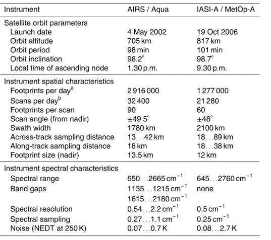
A instrument onboard MetOp-A, which is referred to as IASI on MetOp in this paper. The Aqua and MetOp orbit parameters as well as the spatial and spectral measure-ment characteristics of AIRS and IASI are summarized in Table 1. Both Aqua and MetOp operate in nearly polar, sun-synchronous orbits. The orbit altitudes are 705 and 817 km, respectively. Both satellites have an orbit period of about 100 min and an

or-25

(7)

AMTD

7, 8415–8464, 2014

L. Hoffmann et al.

Title Page

Tables Figures

◭ ◮

Back Close

Full Screen / Esc

Discussion

P

a

per

|

Discus

sion

P

a

per

|

Discussion

P

a

per

|

Discussion

P

a

per

|

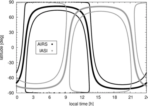
The individual local times of the Aqua and MetOp orbits as a function of latitude are compared in Fig. 1. Both satellites provide coverage at fixed local times. The Equator-crossing of the ascending orbits occurs around 1.30 p.m. for Aqua and 9.30 p.m. for MetOp, i. e., the ascending orbits provide daytime measurements for AIRS and night-time measurements for IASI. For the descending orbits it is the reverse. At high latitudes

5

there is a quick transition in local time.

AIRS and IASI both measure infrared radiance spectra from the earth’s atmosphere in the nadir and sub-limb observation geometry. AIRS applies a rotating mirror to carry out scans in the across-track direction. A scan consists of 90 footprints and covers an across-track distance of 1780 km on the ground. The along-track distance between two

10

scans is 18 km. The across-track sampling distance varies between 13 km at nadir and 42 km at the scan extremes. The footprint size is 13.5 km at nadir. IASI has nearly the

same maximum scan angle as AIRS (about_±50◦), but due to the larger orbit altitude the

IASI swath covers an across-track distance of 2100 km. A nominal IASI scan line covers 30 scan positions, and for each of these scan positions IASI takes measurements in

15

a 2_×2 block of footprints. For this study we rearranged the 30_×2_×2 footprints from an

individual IASI scan into a 60_×2 (across-track_×along-track) pattern to get a sampling

grid similar to AIRS. However, the IASI scan pattern is more irregular than the AIRS

scan pattern because there is a larger distance between each 2_×2 block than inside

a 2_×2 block. The across- and along-track sampling distances of IASI vary between

20

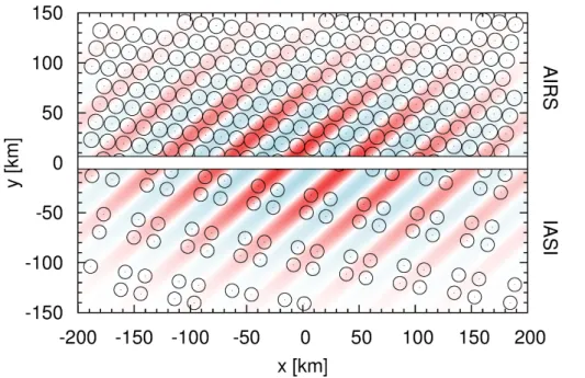
18 and 89 km and 18 and 38 km, respectively. The footprint size is 12 km at nadir. The AIRS and IASI scan patterns are illustrated in Fig. 2. The plot shows that spatial sampling and resolution may have a significant impact on observations of short-scale

gravity waves. AIRS measures spectra for 2.9 million footprints day−1. IASI provides

data for 1.3 million footprints day−1.

25

Both AIRS and IASI provide hyperspectral mid infrared radiance data. AIRS employs

a di_ffraction grating spectrometer and a set of 17 linear arrays of HgCdTe detectors for

(8)

AMTD

7, 8415–8464, 2014

L. Hoffmann et al.

Title Page

Tables Figures

◭ ◮

Back Close

Full Screen / Esc

Discussion

P

a

per

|

Discus

sion

P

a

per

|

Discussion

P

a

per

|

Discussion

P

a

per

λ/∆λ=1200. The noise equivalent delta temperature (NEDT) at 250 K scene

tempera-ture varies between 0.07 and 0.7 K. The processing of the instrument raw data into cali-brated radiance spectra (Level-1B data) and the validation of these data are discussed by Aumann et al. (2000, 2003), Pagano et al. (2003, 2008), and Elliott et al. (2013). The IASI instrument uses a Fourier-transform spectrometer and 3 detector packages

5

for radiance measurements between 3.62 and 15.5 µm. It covers nearly the same spec-tral range as AIRS, but does not have band gaps. The IASI spectra are apodized with

a Gaussian spectral response function (Level-1C data) and have 0.25 cm−1 spectral

sampling and 0.5 cm−1 spectral resolution. The IASI NEDT varies between 0.08 and

2.7 at 250 K scene temperature. Data processing and validation of IASI radiance data

10

are discussed by Simeoni et al. (2004), Blumstein et al. (2007), Illingworth et al. (2009), and Larar et al. (2010).

2.2 Gravity wave analysis

Our study of stratospheric gravity waves based on AIRS and IASI radiance

mea-surements follows the approach of Hoffmann and Alexander (2010) and Hoffmann

15

et al. (2013). In particular, we analyze the 4.3 µm CO₂ fundamental band, which

be-comes optically thick in the middle stratosphere and provides direct information on stratospheric temperatures. For each satellite footprint we calculate the spectral mean

brightness temperature over two spectral ranges from 2322.5 to 2346.0 cm−1_{and from}

2352.5 to 2367.0 cm−1. The small gap between these two ranges was excluded as it

20

contains channels that include signals from the troposphere.

As an example of the influence of stratospheric gravity waves on individual AIRS and IASI measurements, Fig. 3 shows spectra measured by AIRS and IASI during a mountain wave event on 2 August 2010 near the Antarctic Peninsula. This event will be presented in more detail in Sect. 3.1. To simplify the comparison, we convolved the

25

high-resolution IASI spectra with a Gaussian spectral response function with 1.9 cm−1

(9)

AMTD

7, 8415–8464, 2014

L. Hoffmann et al.

Title Page

Tables Figures

◭ ◮

Back Close

Full Screen / Esc

Discussion

P

a

per

|

Discus

sion

P

a

per

|

Discussion

P

a

per

|

Discussion

P

a

per

|

latitude, but separated by about 100 km zonal distance (about half the wavelength of the

mountain wave). As can be seen on the plots the mountain wave is causing di_fferences

of up to 5 K in the 4.3 µm brightness temperatures.

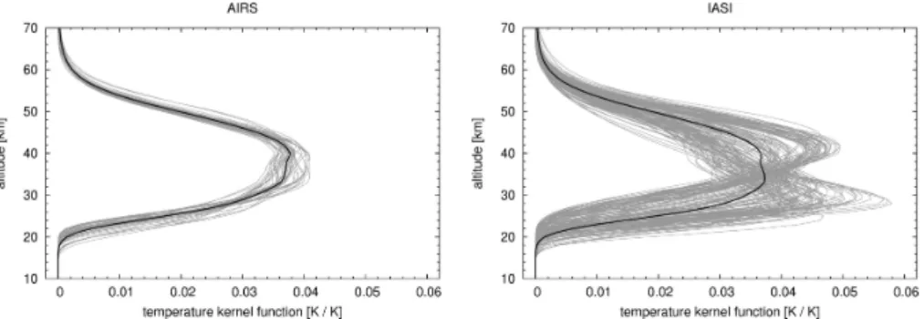
The spectral ranges used in this analysis were initially selected for AIRS, based on the similarity of their temperature kernel functions. Figure 4 compares the individual

5

and spectral mean temperature kernel functions for AIRS and IASI within the selected spectral ranges. In contrast to AIRS, the IASI kernel functions show substantial vari-ation in peak height and width. The diversity of the AIRS and IASI kernel functions is

due to the different spectral resolutions of both instruments at 4.3 µm. IASI has better

spectral resolution and can resolve individual CO₂ lines. As a consequence, diff

er-10

ences in optical depth between line centers and line wings become visible in the kernel functions. However, as we are analyzing spectral mean radiances, only the spectral mean kernel functions of both instruments are of further interest. Figure 4 shows that the spectral mean kernel functions of AIRS and IASI are quite similar. They both have a broad maximum in sensitivity at 30 to 40 km altitude and a full-width at half-maximum

15

of about 25 km. This means that AIRS and IASI provide similar vertical coverage re-garding the gravity wave observations at 4.3 µm. Note that the sensitivity to tempera-ture drops to near zero below 20 km altitude. Tropospheric emissions from interfering species like water vapor, from clouds, or from the surface are generally not expected to influence the 4.3 µm measurements. One notable exception is scenes with very large

20

contrasts between land- and sea-surface temperatures (up to 40 K in the daytime), which are found near the coasts of desert areas, in particular.

A major objective of this study is a statistical comparison of AIRS and IASI 4.3 µm brightness temperature variances due to stratospheric gravity wave activity. The ob-served 4.3 µm brightness temperatures are mainly composed of contributions from

25

three sources. These sources are: (i) slowly varying background signals, (ii) gravity

waves, and (iii) noise. Accordingly, the total brightness temperature variance σ_tot2 is

given by

(10)

AMTD

7, 8415–8464, 2014

L. Hoffmann et al.

Title Page

Tables Figures

◭ ◮

Back Close

Full Screen / Esc

Discussion

P

a

per

|

Discus

sion

P

a

per

|

Discussion

P

a

per

|

Discussion

P

a

per

with background variance σ_bg2 , gravity wave variance σ_gw2 , and noise variance σ_noise2 .

In order to extract the gravity wave signals we must first remove the background sig-nals. The background signals are associated with large-scale gradients in temperature with latitude and planetary-scale waves. Another strong background signal is the

“limb-brightening effect” that refers to an increase in radiance with increasing scan angle due

5

to elongated atmospheric ray paths. The background signals are removed by means of a local “detrending” procedure, which was described in detail by Wu (2004), Eckermann et al. (2006), and Alexander and Barnet (2007). In this procedure the background is es-timated as a 4th-order polynomial fit in the across-track direction for each scan.

Bright-ness temperature perturbations are calculated as di_fferences from the polynomial fit.

10

Note that additional along-track smoothing of the background was not considered here. We found that along-track smoothing can introduce problems in regions where there are strong latitudinal gradients in the temperature field, e. g., at the polar vortex edge.

Both the temperature kernel functions and the detrending procedure influence the sensitivity of the AIRS and IASI gravity wave observations. Figure 5 shows the

sen-15

sitivity of the 4.3 µm brightness temperature variances to wave perturbations with dif-ferent vertical and horizontal wavelengths. The sensitivity to vertical wavelength was determined by convoluting vertical temperature profiles representing wave perturba-tions with the kernel funcperturba-tions and by calculating the ratio of the variance of the result-ing brightness temperature perturbations for all wave phases to their overall maximum.

20

Likewise, sensitivity to horizontal wavelengths was determined by applying the detrend-ing procedure on wave packages in the across-track direction and by calculatdetrend-ing the

ratio of the variances of the detrended perturbations for different wave phases to their

overall maximum. These calculations show that the sensitivity of both instruments first exceeds a level of 1 % for vertical wavelengths larger than 28 km, and that it exceeds

25

(11)

AMTD

7, 8415–8464, 2014

L. Hoffmann et al.

Title Page

Tables Figures

◭ ◮

Back Close

Full Screen / Esc

Discussion

P

a

per

|

Discus

sion

P

a

per

|

Discussion

P

a

per

|

Discussion

P

a

per

|

range for both instruments. For vertical wavelengths larger than 30 km AIRS and IASI

provide the same sensitivity, with relative di_fferences being less than 4 %.

Concerning the sensitivity to horizontal wavelengths, IASI was found to be more sen-sitive than AIRS at wavelengths longer than 600 km. This is due to the broader swath of IASI that allows longer horizontal wavelengths to be seen. The sensitivity drops below

5

90 % at horizontal wavelengths of 730 km for AIRS and 870 km for IASI. It drops below 10 % at 1400 km for AIRS and 1700 km for IASI. Note that the calculations shown in Fig. 5 consider only the spatial sampling, but not the spatial resolution of AIRS and IASI. The sensitivity to short horizontal wavelengths is not represented. The sensitiv-ity to short horizontal wavelengths in both AIRS and IASI is limited by the footprint

10

sizes, which are 13.5 and 12 km, respectively. Therefore IASI provides slightly better horizontal resolution, whereas AIRS has finer sampling. IASI can be more sensitive to short-scale wave perturbations, but the coarser and more irregular scan pattern can

make it di_fficult to identify coherent wave patterns. See Fig. 2 for illustration.

Careful characterization of instrument and scene noise is important for gravity wave

15

analyses as noise can contribute significantly to observed brightness temperature vari-ances. An advantage of the 4.3 µm waveband analyzed here is that large numbers of channels can be averaged to obtain low-noise data products. Our analysis is based on spectral mean brightness temperatures from 42 channels for AIRS and 154 channels for IASI. However, note that the noise reduction for neither AIRS nor IASI follows a strict

20

(1/√n)-scaling law (with nbeing the number of channels), as both instruments have

spectrally correlated noise components. For AIRS correlated noise is introduced as all pixels within a detector module share common circuitry. Correlated noise up to 50 % of the nominal noise was identified in some detector modules (Pagano et al., 2008). For IASI correlated noise is introduced by the apodization of the radiance spectra.

25

(12)

AMTD

7, 8415–8464, 2014

L. Hoffmann et al.

Title Page

Tables Figures

◭ ◮

Back Close

Full Screen / Esc

Discussion

P

a

per

|

Discus

sion

P

a

per

|

Discussion

P

a

per

|

Discussion

P

a

per

measurements along the satellite orbits into individual boxes of 90_×90 and 60_×60

footprints, respectively (about 2000 km_×2000 km in both cases). Individual noise

esti-mates for each box were obtained by convoluting the spectral mean 4.3 µm brightness

temperature data with a 3_×3 pixel filter mask to remove image structures. Noise

esti-mates were obtained by calculating the variance of the filtered data. Note that the

es-5

timator of Immerkær (1996) perceives thin lines as noise, i. e., plane waves with short wavelengths are potentially misinterpreted as noise. However, as shown below, we

ap-plied the analysis separately to hundreds of boxes for both AIRS and IASI in di_fferent

regions and seasons and found that there are only few outliers of exceptionally high noise that are likely related to that problem. For each of the boxes we also calculated

10

the mean brightness temperature to get an estimate of the scene temperature.

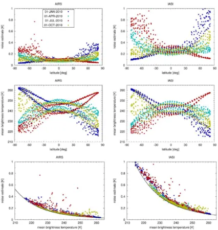
Figure 6 shows our noise estimates for the 4.3 µm spectral mean brightness temper-ature measurements of AIRS and IASI. For both instruments we found a substantial

variation in the noise with latitude and season, with di_fferences of up to a factor of

10. This latitudinal and seasonal variation is due to the dependence of the NEDT on

15

scene temperature. The NEDT decreases with increasing scene temperatures, i. e., it becomes lowest in polar summer (maximum scene temperatures) and highest in polar winter (minimum scene temperatures). Furthermore, Fig. 6 reveals day- and nighttime

differences of up to 50 % in noise at low and mid latitudes. Daytime scene temperatures

are up to 10 K higher than nighttime values as the CO₂molecules experience solar

ex-20

citation and get into the state of non-local thermodynamic equilibrium (non-LTE) (e. g., de Souza-Machado et al., 2006). Even though there is substantial variability in the individual noise values, scatter plots of noise vs. scene temperature reveal compact correlations for both AIRS and IASI, independent of latitude, season, and time of day. To parametrize these compact correlations, we fitted noise scaling curves based on the

25

Planck functionBand its inverseB−1_{to the data,}

NEDT (T_sc)=B−1_[_B₍_T

(13)

AMTD

7, 8415–8464, 2014

L. Hoffmann et al.

Title Page

Tables Figures

◭ ◮

Back Close

Full Screen / Esc

Discussion

P

a

per

|

Discus

sion

P

a

per

|

Discussion

P

a

per

|

Discussion

P

a

per

|

Here we assumed that the NEDT varies with scene temperatureT_scwhereas the noise

equivalent spectral radiance (NESR) is constant. The NESR was obtained by fitting the

NEDT_refat a given reference temperatureT_ref,

NESR =B(Tref+NEDTref)−B(Tref). (3)

By fitting to the minimum noise estimates at different scene temperatures we found

5

noise scaling curves that are defined by NEDT_ref₌0.059 K for AIRS and NEDT_ref₌

0.15 K for IASI, both atT_ref=250 K (see Fig. 6). This means the IASI noise at 4.3 µm

is about a factor 2.4 larger than the AIRS noise. In other parts of this study we applied the noise scaling curves to determine the noise based on given scene temperatures rather than estimating it individually for each scene. This provides stable results even

10

in scenes with strong wave activity where direct noise estimation from the scene data may fail.

Finally, note that we had to carefully screen the AIRS and IASI data for outliers. In particular in the IASI data we found a few individual footprints with unrealistically large deviations in the 4.3 µm brightness temperatures compared to their direct

neigh-15

bours. Such individual outliers distort the polynomial fit for background estimation and subsequently cause substantial errors in variance estimation. For both AIRS and IASI we evaluated the operational data quality flags to exclude footprints with degraded data quality. However, for IASI we found that the operational data quality flags do not capture all outliers in the 4.3 µm radiances. In some scenes with very low brightness

tempera-20

tures, which are often related to deep convective clouds in the line of sight, calibration procedures can fail and physically unrealistic spectra are produced. We identified such spectra by means of a correlation test. We calculated the Pearson linear correlation

co-efficientρbetween the test spectrum and a mid-latitude clear-air reference spectrum in

the spectral interval from 2320 to 2370 cm−1_{. If} _ρ_{dropped below a latitude-dependent}

25

threshold (0.0 at the equator, ₋0.7 at the poles, and linear interpolation in between)

(14)

AMTD

7, 8415–8464, 2014

L. Hoffmann et al.

Title Page

Tables Figures

◭ ◮

Back Close

Full Screen / Esc

Discussion

P

a

per

|

Discus

sion

P

a

per

|

Discussion

P

a

per

|

Discussion

P

a

per

outlier filters remove about 1.5 % of the IASI footprints. AIRS is much less affected by

outliers.

3 Results

3.1 Case study of mountain waves near the Antarctic Peninsula

We selected a mountain wave event near the Antarctic Peninsula as our first case study

5

for comparison of AIRS and IASI gravity wave observations. The Antarctic Peninsula is the northernmost part of the mainland of Antarctica. It is approximately 1300 km long

and stretches from 75 to 63◦S and from 76 to 57◦W. The Antarctic Peninsula is a

moun-tain chain, with its highest peak rising to 2800 m. Cape Horn, the southern tip of South America, is about 1000 km north of the peninsula. A strong circumpolar flow in the

win-10

tertime troposphere and stratosphere is a unique feature of Antarctica. The Antarctic

Peninsula and Cape Horn create a funneling effect, which directs surface winds into

the Drake Passage. Based on this setting, the Antarctic Peninsula becomes a major orographic source for gravity waves. Many observational studies demonstrated that the Antarctic Peninsula is indeed a hotspot of stratospheric gravity wave activity (Wu and

15

Jiang, 2002; Jiang et al., 2006; Baumgaertner and McDonald, 2007; Vincent et al.,

2007; Hertzog et al., 2008; Alexander et al., 2009b; Hoffmann et al., 2013). Orographic

waves over the Antarctic Peninsula have also been extensively studied by means of mesoscale model simulations (Plougonven et al., 2008; de la Torre et al., 2012; Noel and Pitts, 2012; Orr et al., 2014). Mountain waves generated by the peninsula are of

20

interest not only because of their impact on atmospheric dynamics, but also because they can trigger the formation of polar stratospheric clouds. This is most relevant in early and late winter, when synoptic-scale temperatures are above formation threshold temperatures (Höpfner et al., 2006; Eckermann et al., 2009; McDonald et al., 2009; Lambert et al., 2012).

(15)

AMTD

7, 8415–8464, 2014

L. Hoffmann et al.

Title Page

Tables Figures

◭ ◮

Back Close

Full Screen / Esc

Discussion

P

a

per

|

Discus

sion

P

a

per

|

Discussion

P

a

per

|

Discussion

P

a

per

|

Mountain waves over the Antarctic Peninsula often last for a day or longer. They are associated with substantial stratospheric temperature perturbations and with horizontal wavelengths of several hundred kilometers. Mountain waves are stationary, i.e., they remain in a constant position with time. This type of gravity wave is well suited to ob-servation with infrared nadir sounders. Figure 7 shows 4.3 µm brightness temperature

5

perturbations for selected AIRS and IASI overpasses of the Antarctic Peninsula dur-ing a mountain wave event on 2–3 August 2010. Note that due to the high latitude of the Antarctic Peninsula and also to the broad swath of both instruments we typically obtain useful observations from four rather than two satellite overpasses per day. The brightness temperature perturbation maps illustrate that both instrument are clearly

ca-10

pable of observing this particular mountain wave event and that together they provide a consistent picture of its temporal development.

There is one particularly remarkable example of coincident AIRS and IASI observa-tions on 2 August 2010, when two overpasses were separated by only a few minutes, occurring at 03:54 and 03:57 UTC. The wave patterns observed by the two

instru-15

ments show excellent agreement (Fig. 7). We performed a spectral analysis for the two satellite overpasses using the S-Transform (Stockwell et al., 1996), and the method de-scribed by Alexander and Teitelbaum (2007). This approach has the distinct advantage of providing spectral information on a variety of local scales. Results are presented in Fig. 8. The patterns found in the wave amplitudes clearly coincide with the wave

20

patterns in the brightness temperature perturbations. The maximum wave amplitudes are up to 3.9 K for IASI and 5.2 K for AIRS. Considering only data points with wave amplitudes larger than 1 K, the amplitude-weighted mean horizontal wavelengths are 170 km for IASI and 130 km for AIRS. These results from the spectral analyses show

that both the AIRS and IASI measurements are very similar. The remaining differences

25

(16)

AMTD

7, 8415–8464, 2014

L. Hoffmann et al.

Title Page

Tables Figures

◭ ◮

Back Close

Full Screen / Esc

Discussion

P

a

per

|

Discus

sion

P

a

per

|

Discussion

P

a

per

|

Discussion

P

a

per

3.2 Case study of orographic waves near the Kerguelen Islands and Heard Island

For our second case study, we present orographic waves near Kerguelen Islands

(49◦_{S, 70}◦_{E) and Heard Island (53}◦_{S, 74}◦_{E). Gibbs (1945) provides a geographical}

report on these remote islands in the Southern Indian Ocean. The Kerguelen Islands,

5

also known as the Desolation Islands, are more than 3300 km away from the nearest populated location. The main island, Grande Terre, extends 150 km east to west and 120 km north to south and is surrounded by numerous smaller islands. The highest point on Grand Terre is Mont Ross (1850 m). Heard Island is located about 470 km

southeast of the Kerguelen Islands. Heard Island has an area of 370 km2. Its highest

10

summit is Mawson Peak (2745 m), an active volcano. The climate of the Kerguelen Islands and Heard Island is subpolar oceanic, tempered by a maritime setting. The islands are located in the “Roaring Forties” and “Furious Fifties”. Their west coasts

receive continuous winds of 5–10 m s−1_{; wind gusts of 40 –50 m s}−1_{are common.}1

Satellite observations of orographic gravity waves generated by flow over small

is-15

lands in the southern oceans have been discussed in several studies (Wu et al., 2006;

Alexander et al., 2009a; Alexander and Grimsdell, 2013; Ho_ffmann et al., 2013). In

particular, Alexander and Grimsdell (2013) examined the occurrence frequencies of these waves in the stratosphere above 14 islands based on two years of AIRS ob-servations. Their study showed that waves commonly occur in the May to September

20

season, though not every day. Differing seasonal variations became evident at different

islands, but the seasonal variations were closely related to latitude and prevailing wind patterns. Alexander and Grimsdell (2013) found that stratospheric winds have a

first-order limiting effect on satellite observations of the island mountain waves. Surface

wind direction and island orographic relief have a secondary influence on the wave

oc-25

(17)

AMTD

7, 8415–8464, 2014

L. Hoffmann et al.

Title Page

Tables Figures

◭ ◮

Back Close

Full Screen / Esc

Discussion

P

a

per

|

Discus

sion

P

a

per

|

Discussion

P

a

per

|

Discussion

P

a

per

|

In this case study we focus on observations of orographic waves near the Kerguelen Islands and Heard Island on 23–24 June 2010. Figure 9 shows brightness temper-ature perturbation maps of selected AIRS and IASI overpasses. The maps illustrate that both AIRS and IASI are clearly capable of observing this type of wave event. How-ever, note that these observations are more challenging for IASI, compared to mountain

5

wave events at the Antarctic Peninsula, because the horizontal wavelengths are usually much shorter. To illustrate this an AIRS map for another wave event on 24 June 2010, 20:15 UTC is given in Fig. 9. This map reveals orographic waves with horizontal wave-lengths as short as 70 km northeast of the Kerguelen Islands. Such waves would be

difficult to observe and identify as a coherent wave pattern with IASI due to its fairly

10

coarse and irregular sampling pattern.

Figure 9 also shows maps of local variances that measure the variance within circles

of 100 km radius (see Hoffmann and Alexander, 2010; Hoffmann et al., 2013). Both

instruments recorded strong gravity wave activity in the stratosphere, with maximum

local variances up to 28 K2 for IASI and 6 K2 for AIRS at the Kerguelen Islands and

15

7 K2 for IASI and 4 K2 for AIRS at Heard Island. We think that the larger variances of

IASI are partly due to the better horizontal resolution of IASI (i. e., its smaller footprint size), which makes the instrument more sensitive to large wave amplitudes from

short-scale waves. We also analyzed this particular event for visibility effects, i. e., changes

in sensitivity due to wavelength changes along the line-of-sight depending on the scan

20

angle. However, we found that this does not play a role in this case study. The combined AIRS and IASI data indicate that the island mountain waves are rather variable in time. In many situations we found strong wave events only in single AIRS or IASI overpasses, but not in subsequent satellite overpasses.

3.3 Case study of convective waves during the North American

25

thunderstorm season

(18)

AMTD

7, 8415–8464, 2014

L. Hoffmann et al.

Title Page

Tables Figures

◭ ◮

Back Close

Full Screen / Esc

Discussion

P

a

per

|

Discus

sion

P

a

per

|

Discussion

P

a

per

|

Discussion

P

a

per

begins in late April and continues until early September. The meteorological situation is characterized by a southerly low-level jet shifting north, i. e., warm and moist air from the Gulf of Mexico can invade inner continental regions. The moist air feeds thunder-storms, which develop in advance of Pacific cold fronts. The thunderstorms cluster in swaths, oriented southwest to northeast, and move towards the northeast ahead of

5

the fronts. Deep convection related to thunderstorms is an important source for gravity waves. Convective waves in the summer mid and high latitudes may play a leading role in driving the stratospheric Brewer–Dobson circulation in the summer hemisphere

(Alexander and Rosenlof, 1996). Hoffmann and Alexander (2010) analyzed the

occur-rence frequency of convective waves during the North American thunderstorm season

10

based on AIRS data. This shows that more than 95 % of the observed gravity waves

in a core region over the North American Great Plains (36 to 46◦N, 88 to 98◦W) are

associated with deep convection. The occurrence frequency of these convective waves varies with time of day. Stronger activity is observed for the descending orbits of AIRS,

which are measured at a local time of 1.30 p.m. The di_fferent local times of the AIRS

15

and IASI orbits (Fig. 1) bear the opportunity to study the temporal development of these convective waves in more detail.

In this case study we focus on a convective wave event on 16 June 2009 (Fig. 10). We present four satellite overpasses within a time period of 21 h. Convective waves are observed during two overpasses, at 03:12 UTC by IASI and at 08:01 UTC by AIRS.

20

The convective waves can be identified in the perturbations maps based on their semi-circular shape. Note that the observed wave fronts preferably propagate east-ward, corresponding to strong westerly background winds that foster the propagation of waves with long vertical wavelengths in that direction. Those long vertical wavelengths are best visible to AIRS and IASI (Sect. 2.2). Figure 10 also shows maps of 8.1 µm

25

(1231 cm−1_{) brightness temperatures. These maps allow identification of deep}

con-vection based on low brightness temperatures (e. g., Ho_ffmann and Alexander, 2010;

(19)

AMTD

7, 8415–8464, 2014

L. Hoffmann et al.

Title Page

Tables Figures

◭ ◮

Back Close

Full Screen / Esc

Discussion

P

a

per

|

Discus

sion

P

a

per

|

Discussion

P

a

per

|

Discussion

P

a

per

|

of the semi-circular wave patterns (40◦_{N, 95}◦_{W), indicating that the waves are indeed}

convectively driven and that this convective system is the source.

Note that this case study presents one of the most distinct cases of coincident con-vective wave observations with AIRS and IASI that we could identify during the time

period from 2008 to 2012. Convective waves are very di_fficult for both AIRS and IASI to

5

identify, because these waves usually have much weaker amplitudes than orographic waves and they are much more variable in time due to the variability of the convec-tive sources. Convecconvec-tive wave observations are usually noise-limited, in particular for IASI. The IASI observations sometimes reveal fluctuating strong brightness tempera-ture perturbations close to the center of the convective waves, which may be related

10

to its better horizontal resolution. AIRS shows smaller perturbations, but the wave pat-terns are more coherent due to the better horizontal sampling.

3.4 Temporal patterns of stratospheric gravity wave activity

In this section we describe statistical analyses of the stratospheric gravity wave vari-ances from AIRS and IASI. The analyses span the time period from January 2008 to

15

December 2012, which has nearly complete coverage by both AIRS and IASI. During

that time period AIRS measured about 5.3_×109 and IASI about 2.3_×109 radiance

spectra. Statistical sampling errors can be neglected in most cases due to the large

number of measurements. An exception is at high latitudes (beyond_±85◦), where the

number of measurements decreases rapidly. This region is excluded from our analysis.

20

As gravity wave activity varies with local time, the analyses are carried out separately for the ascending orbits of AIRS and descending orbits of IASI (daytime data) as well as the descending orbits of AIRS and ascending orbits of IASI (nighttime data). To il-lustrate our analyses, Fig. 11 shows time series of the daily mean, zonal mean 4.3 µm brightness temperature background levels, noise estimates, and gravity wave variances

25

for 1◦_{latitude bins from the IASI nighttime data.}

(20)

AMTD

7, 8415–8464, 2014

L. Hoffmann et al.

Title Page

Tables Figures

◭ ◮

Back Close

Full Screen / Esc

Discussion

P

a

per

|

Discus

sion

P

a

per

|

Discussion

P

a

per

|

Discussion

P

a

per

(below_±25◦_{) the temperature variations were small (up to}

±5 K), but the variability

in-creased towards polar latitudes (up to_±30 K). A remarkable feature of the time series

is the stratospheric sudden warmings (e. g., Charlton and Polvani, 2007; Ayarzagüena et al., 2011), which increase background temperatures by up to 40 K in the polar re-gions and decrease them by 5–10 K at low and mid latitudes. Comparing IASI

day-5

and nighttime data (not shown), we found the daytime background temperatures were

biased high by up to 10 K within _±60◦ _{latitude. This bias is attributed to non-LTE}

(Sect. 2.2) and diminishes towards the poles. Comparing AIRS and IASI (not shown), we found excellent agreement in the background temperatures. At nighttime the AIRS

and IASI background temperatures typically di_ffer less than_±1 K at all latitudes. During

10

the daytime AIRS is typically about 2–3 K larger than IASI, which we attribute to the

different local times of the measurement and non-LTE.

Figures 11 and 12 show time series of noise variances for AIRS and IASI, which we calculated from the 4.3 µm background temperatures and the noise scaling functions presented in Sect. 2.2. Depending on latitude, season, and time of day, the noise

vari-15

ances can fluctuate by 2–3 orders of magnitude, i. e., from 0.00076 to 0.60 K2for AIRS

and from 0.0046 to 2.8 K2for IASI. Being anti-correlated with background temperatures,

the lowest noise is found in the polar summer and the highest noise is found in the

po-lar winter. Day- and nighttime differences in background temperatures due to non-LTE

map into noise as well, with nighttime noise variances typically being 2–5 times larger

20

than daytime noise variances at low and mid latitudes. Comparing AIRS and IASI, it is found that IASI noise variances are typically 3–6 times larger than AIRS noise

vari-ances. Individual gravity wave events may yield local variances of 10 K2or more (e. g.,

Sect. 3.2). Zonally or seasonally averaged gravity wave variances are typically lower

(on the order of 1 K2, see below). The large variation of the 4.3 µm noise with latitude,

25

season, and time of day found here demonstrates that a careful characterization and noise correction in statistical analyses of gravity wave variances is mandatory.

(21)

AMTD

7, 8415–8464, 2014

L. Hoffmann et al.

Title Page

Tables Figures

◭ ◮

Back Close

Full Screen / Esc

Discussion

P

a

per

|

Discus

sion

P

a

per

|

Discussion

P

a

per

|

Discussion

P

a

per

|

wave activity, including a strong cycle with maxima in winter mid and high latitudes and a weaker cycle with maxima in summer low latitudes. The high latitude winter cycle is mostly related to orographic wave activity and the polar jet. We found daily maxima

of the zonal mean gravity wave variances up to 2 K2 at mid and high latitudes in both

hemispheres. In contrast, the low latitude summer cycle is related to convection and

5

the subtropical jet. The daily maxima of the summer cycle are typically a factor 20–30 smaller than the maxima of the winter cycle. Note that the zonal winds in the middle stratosphere have a strong influence on the AIRS and IASI gravity wave observations. Strong winds foster the propagation of gravity waves with long vertical wavelengths, which are best visible to the nadir sounders (Sect. 2.2). Figure 11 shows a time series

10

of zonal mean zonal winds at 6.8 hPa (about 35 km, at the AIRS and IASI observation level) from the European Centre for Medium-Range Weather Forecast ERA-Interim reanalysis (Dee et al., 2011). The time series of the gravity wave variances and the zonal winds are clearly correlated, with the winter cycle maxima in wave activity being associated with strong westerlies and the summer cycle maxima being associated with

15

prevailing easterlies.

Although the temporal patterns of gravity wave activity from AIRS and IASI are in

agreement, Fig. 12 reveals some di_fferences. The IASI variances are systematically

larger than the AIRS variances, with the largest di_fferences being found in the

win-ter cycle maxima (up to 1 K2). In contrast, at equatorial latitudes the AIRS and IASI

20

variances agree well, with di_fferences below_±0.015 K2. As the observed wave activity

at equatorial latitudes is close to zero, the small di_fferences found here relate to the

accuracy of the AIRS and IASI noise corrections and indicate that these corrections were carried out properly. Note also that the noise corrections remove the day- and

nighttime di_fferences. To quantify the remaining di_fferences between AIRS and IASI,

25

we determined the linear scaling factor between the gravity wave variances,

(22)

AMTD

7, 8415–8464, 2014

L. Hoffmann et al.

Title Page

Tables Figures

◭ ◮

Back Close

Full Screen / Esc

Discussion

P

a

per

|

Discus

sion

P

a

per

|

Discussion

P

a

per

|

Discussion

P

a

per

This is a combined value for and nighttime data. A separate analysis for

day-or nighttime yields similar scaling factday-ors (with di_fferences less than 5 %). Figure 12

also reveals systematic differences between day- and nighttime data, with nighttime

variances being larger than daytime variances. The linear scaling factor between the gravity wave variances is

5

cdn=1.315±0.062. (5)

This is a combined value based on AIRS data, scaled to IASI levels by multiplying with

c_ai, and unaltered IASI data. A separate analysis for AIRS and IASI again yields similar

scaling factors (with differences less than 5 %).

3.5 Spatial patterns of stratospheric gravity wave activity

10

In this section we discuss the spatial distributions of the AIRS and IASI gravity wave

variances in di_fferent seasons. Figures 13 and 14 show five-year averages (2008–

2012) of monthly mean variances in January and July, respectively. The variances were

calculated on a 1◦

×1◦ horizontal grid. We scaled the AIRS data with the global factor

c_ai and the daytime data with the global factorc_dnto compensate for some of the

sys-15

tematic differences discussed in Sect. 3.4. The comparison of the scaled data shows

good agreement in many cases. The remaining differences are mostly below _±0.2 K.

Larger di_fferences are found only in few locations with exceptionally strong gravity wave

activity. In these cases the global correction of the scaling approach may not be suited for the specific local gravity wave spectra. Note that there is some statistical uncertainty

20

due to the limited length of the time series, in particular in cases where the variances are mainly determined by few, exceptionally strong events. However, the remaining

differences are certainly linked to local time variation of the gravity wave sources as

well.

The monthly maps presented in Figs. 13 and 14 reveal distinct features of

strato-25

(23)

AMTD

7, 8415–8464, 2014

L. Hoffmann et al.

Title Page

Tables Figures

◭ ◮

Back Close

Full Screen / Esc

Discussion

P

a

per

|

Discus

sion

P

a

per

|

Discussion

P

a

per

|

Discussion

P

a

per

|

strong westerly winds (exceeding 20–40 m s−1). In the Southern Hemisphere wave

ac-tivity is more zonally symmetric. A notable exception is found near the Andes and the Antarctic Peninsula, where wave activity is up to a factor 10 larger than the zonal mean.

Another exception is found over the southern Atlantic and Indian Ocean (50–70◦_{S, 0–}

120◦E), which correlates with even stronger stratospheric winds (>80 m s−1). In the

5

Northern Hemisphere the observed distribution of gravity wave activity is zonally asym-metric due to the asymmetry in the orography and background winds. The largest wave activity is observed over the Atlantic Ocean and Europe. In the summer hemispheres we observe weaker local maxima at low and mid latitudes that coincide with regions

of convective activity and that are confined by easterly winds exceeding ₋20 m s−1.

10

This includes the North American Great Plains and South-East Asia in boreal sum-mer (July) and central South Asum-merica, south Africa, and northern Australia in austral summer (January). Due to the high horizontal resolution, AIRS and IASI are both well capable of resolving small-scale hotspots of stratospheric gravity wave activity, which

are discussed in detail by Hoffmann et al. (2013).

15

4 Discussion and conclusions

In this study we performed an intercomparison of 4.3 µm brightness temperature mea-surements of AIRS and IASI to assess how stratospheric gravity wave observations of both instruments relate to each other. The analyses were based on spectral mean radi-ances rather than on spectrally resolved data. The main advantages of spectral

averag-20

ing are that it reduces noise and that it makes the measurements comparable in terms of vertical coverage. A disadvantage is that altitude information gets lost, in particular for IASI with its high spectral resolution. In summary, we found that AIRS and IASI are both well capable of observing stratospheric gravity waves with long vertical and short horizontal wavelengths. These waves are believed to be rather important as they can

25

(24)

AMTD

7, 8415–8464, 2014

L. Hoffmann et al.

Title Page

Tables Figures

◭ ◮

Back Close

Full Screen / Esc

Discussion

P

a

per

|

Discus

sion

P

a

per

|

Discussion

P

a

per

|

Discussion

P

a

per

are related to orographic sources and the polar jet, as well as low and mid latitudes in summer, where convective sources play an important role. Stratospheric gravity wave activity was mostly observed in regions with background zonal winds exceeding wind

speeds of _±20 m s−1. Strong winds foster the propagation of gravity waves with long

vertical wavelengths, which are best visible to the nadir sounders.

5

For gravity wave research it is most promising that AIRS and IASI measure at dif-ferent local times. Combining observations from both instruments provides a clearer picture of the temporal development of individual gravity wave events than a single in-strument alone. The case study for the Antarctic Peninsula showed a mountain wave event that lasted for a period of 48 h. During that time the Antarctic Peninsula was

cov-10

ered by 16 satellite overpasses. On one occasion the AIRS and IASI measurements were separated only by a few minutes’ time and we found that the observed wave pat-terns are in excellent agreement. Furthermore, we also identified cases of orographic waves near isolated islands and convective waves near a mesoscale convective system where AIRS and IASI provided coincident measurements. The case studies revealed

15

distinct advantages of AIRS compared to IASI with respect to the horizontal sampling and resolution of the observations. Finer horizontal sampling of AIRS allows to resolve coherent wave patterns even in case of short-scale waves. In contrast, IASI has better spatial resolution than AIRS and is more sensitive to large amplitudes of short-scale waves. The observed wave patterns may not be as coherent as for AIRS, though, due

20

to the coarser and more irregular sampling pattern of IASI. Another advantage of IASI is its broader swath that reduces data gaps between subsequent measurement track and improves global coverage.

A statistical comparison based on five-year time series (2008–2012) revealed that the IASI gravity wave variances are on average 45 % larger than for AIRS. There are

25

several possible reasons for these differences: (i) IASI can be up to 2.5 times more

sensitive for vertical wavelengths from 10 to 30 km. Although the response in bright-ness temperature variances is quite low at these wavelengths (Fig. 5), this is a

(25)

AMTD

7, 8415–8464, 2014

L. Hoffmann et al.

Title Page

Tables Figures

◭ ◮

Back Close

Full Screen / Esc

Discussion

P

a

per

|

Discus

sion

P

a

per

|

Discussion

P

a

per

|

Discussion

P

a

per

|

sensitivity may be important. (ii) The wider swath width of IASI gives sensitivity to longer horizontal wavelength (Fig. 5) that can contribute to larger variances. (iii) The smaller footprint of IASI (12 km diameter at nadir vs. 13.5 km for AIRS) will give sensitivity to short horizontal wavelength waves near this limit that could contribute to larger vari-ances, even though the coarser sampling of IASI does not permit resolution of such

5

short waves. (iv) IASI noise variances are up to 6 times larger than for AIRS, hence im-perfect noise characterization could still be influencing these results. A specific problem with noise characterization is related to assinging the appropriate scene temperature for each footprint, in particular in scenes with strong variations in radiance. In addition,

we also analyzed day- and nighttime differences and found that gravity wave variances

10

are about 30 % larger at nighttime for both, AIRS and IASI. Part of this di_fference is due

to local time variation of gravity wave sources, such as convection.

Despite the systematic differences, the seasonal and latitudinal distributions of

stratospheric gravity wave activity found here agree well with other climatologies (e. g.,

Jiang et al., 2005; Preusse et al., 2009a; Gong et al., 2012; Ho_ffmann et al., 2013). Our

15

analysis reproduces major features like orography- and jet-related wintertime maxima at mid and high latitudes, low and mid latitude summertime maxima from convective sources, and the most prominent local hotspots of stratospheric gravity waves. We also found good quantitative agreement of the gravity wave variances with the clima-tology of Gong et al. (2012), which is based on 15 µm radiance measurements from

20

AIRS. In their study, Gong et al. (2012, Fig. 4) found maximum zonal mean variances

near 3 hPa (about 40 km) up to 0.3 K2 at 50 to 60◦N and up to 0.1 K2 at 10 to 20◦S in

January 2005. They found even larger maxima in Southern Hemisphere winter (up to

0.5 K2, July 2005), which can also be found in our record.

We recognized that noise is an important contributor to the observed 4.3 µm

bright-25

(26)

AMTD

7, 8415–8464, 2014

L. Hoffmann et al.

Title Page

Tables Figures

◭ ◮

Back Close

Full Screen / Esc

Discussion

P

a

per

|

Discus

sion

P

a

per

|

Discussion

P

a

per

|

Discussion

P

a

per

components into account, which is rather important as we average data from large numbers of channels. For both instruments we found that the 4.3 µm noise variances vary substantially with scene temperature, i. e., by 2 to 3 orders of magnitude. The IASI noise at 4.3 µm is about a factor 2.4 times larger than the AIRS noise. Noise poses a limiting factor for gravity wave observations in cases with low amplitudes, in

particu-5

lar for convective waves.

Previous studies on AIRS may not have taken the large variability of noise with scene temperature fully into account. For instance, in the study of Gong et al. (2012) it was assumed that noise does not vary with location and time. This may have been ap-propriate in their study, because they analyzed 15 µm rather than 4.3 µm brightness

10

temperatures, with weaker dependence of the noise on the scene temperature. Gong et al. (2012) estimated noise directly from the measurements and found that minima occur at summer hemisphere high latitudes, which is confirmed by our results. Wu and Waters (1996) and Wu and Eckermann (2008) point out that the minimum detectable gravity wave variance is directly related to the noise variance. As a consequence, the

15

minimum detection level for the 4.3 µm observations varies substantially with the scene

temperature. The study of Ho_ffmann et al. (2013) presented a detection algorithm for

stratospheric gravity waves that implicitly considered the large noise variation at 4.3 µm. That study used variance thresholds for detection that vary with latitude, season, and time of day.

20

While AIRS has been successfully used in many studies on gravity wave research, IASI data are applied here for the first time for that purpose. Our study indicates that

gravity wave observations from di_fferent hyperspectral infrared nadir sounders such

as AIRS and IASI can be directly related to each other, if instrument-specific

charac-teristics such as different noise levels as well as spatial sampling and resolution are

25