AMTD
6, 2643–2720, 2013SMILES O3 validation
(NICT L2-v215)
Y. Kasai et al.
Title Page
Abstract Introduction
Conclusions References
Tables Figures
◭ ◮
◭ ◮
Back Close
Full Screen / Esc
Printer-friendly Version
Interactive Discussion
Discussion
P
a
per
|
Dis
cussion
P
a
per
|
Discussion
P
a
per
|
Discussio
n
P
a
per
|
Atmos. Meas. Tech. Discuss., 6, 2643–2720, 2013 www.atmos-meas-tech-discuss.net/6/2643/2013/ doi:10.5194/amtd-6-2643-2013
© Author(s) 2013. CC Attribution 3.0 License.
Atmospheric Measurement
Techniques
Open Access
Discussions
Geoscientiic Geoscientiic
Geoscientiic Geoscientiic
This discussion paper is/has been under review for the journal Atmospheric Measurement Techniques (AMT). Please refer to the corresponding final paper in AMT if available.
Validation of stratospheric and
mesospheric ozone observed by SMILES
from International Space Station
Y. Kasai1,2, H. Sagawa1, D. Kreyling1, K. Suzuki1,3, E. Dupuy1,4, T. O. Sato2,1, J. Mendrok5,1, P. Baron1, T. Nishibori6,1, S. Mizobuchi6, K. Kikuchi1, T. Manabe7, H. Ozeki8, T. Sugita4, M. Fujiwara9, Y. Irimajiri1, K. A. Walker10,11, P. F. Bernath12, C. Boone11, G. Stiller13, T. von Clarmann13, J. Orphal13, J. Urban14, D. Murtagh14, E. J. Llewellyn15, D. Degenstein15, A. E. Bourassa15, N. D. Lloyd15,
L. Froidevaux16, M. Birk17, G. Wagner17, F. Schreier17, J. Xu17, P. Vogt17, T. Trautmann17, and M. Yasui1
1
National Institute of Information and Communications Technology (NICT), Koganei, Tokyo, Japan
2
Tokyo Institute of Technology, Yokohama, Kanagawa, Japan
3
The University of Tokyo, Graduate School of Arts and Sciences, Meguro, Tokyo, Japan
4
National Institute for Environmental Studies, Tsukuba, Ibaraki, Japan
5
Lule ˚a University of Technology, Kiruna, Sweden
6
Japan Aerospace Exploration Agency (JAXA), Tsukuba, Japan
7
Osaka Prefecture University, Naka, Sakai, Osaka, Japan
AMTD
6, 2643–2720, 2013SMILES O3 validation
(NICT L2-v215)
Y. Kasai et al.
Title Page
Abstract Introduction
Conclusions References
Tables Figures
◭ ◮
◭ ◮
Back Close
Full Screen / Esc
Printer-friendly Version
Interactive Discussion
Discussion
P
a
per
|
Dis
cussion
P
a
per
|
Discussion
P
a
per
|
Discussio
n
P
a
per
|
8
Toho University, Funabashi, Chiba, Japan
9
Hokkaido University, Kita, Sapporo, Japan
10
University of Toronto, Toronto, Ontario, Canada
11
University of Waterloo, Waterloo, Ontario, Canada
12
Old Dominion University, Norfolk, Virginia, USA
13
Institute for Meteorology and Climate Research (IMK), Karlsruhe Institute of Technology, Karlsruhe, Germany
14
Chalmers University of Technology, G ¨oteborg, Sweden
15
Institute of Space and Atmospheric Studies, University of Saskatchewan, Saskatoon, Canada
16
Jet Propulsion Laboratory (JPL), California Institute of Technology, Pasadena, California, USA
17
German Aerospace Center (DLR), Remote Sensing Technology Institute, Oberpfaffenhofen, Weßling, Germany
Received: 18 February 2013 – Accepted: 25 February 2013 – Published: 18 March 2013
Correspondence to: Y. Kasai ([email protected])
AMTD
6, 2643–2720, 2013SMILES O3 validation
(NICT L2-v215)
Y. Kasai et al.
Title Page
Abstract Introduction
Conclusions References
Tables Figures
◭ ◮
◭ ◮
Back Close
Full Screen / Esc
Printer-friendly Version
Interactive Discussion
Discussion
P
a
per
|
Dis
cussion
P
a
per
|
Discussion
P
a
per
|
Discussio
n
P
a
per
|
Abstract
We observed the diurnal variation of ozone (O3) in the vertical region between 250
and 0.0005 hPa (∼12–96 km) using the Superconducting Submillimeter-Wave
Limb-Emission Sounder (SMILES) on the Japanese Experiment Module (JEM) of the Inter-national Space Station (ISS) between 12 October 2009 and 21 April 2010. The new 4 K
5
superconducting heterodyne receiver technology of SMILES allowed us to obtain a one order of magnitude better signal-to-noise ratio for the O3 line observation compared to past spaceborne microwave instruments. We assessed the quality of the vertical profiles of O3in the 100–0.001 hP (∼16–90 km) region for the SMILES NICT Level 2 product version 2.1.5. The evaluation is based on four components; error analysis;
in-10
ternal comparisons of observations targeting three different instrumental setups for the same O3 625.371 GHz transition; internal comparisons of two different retrieval algo-rithms; and external comparisons for various local times with ozonesonde, satellite and balloon observations (ENVISAT/MIPAS, SCISAT/ACE-FTS, Odin/OSIRIS, Odin/SMR,
Aura/MLS, TELIS). SMILES O3 data have an estimated absolute accuracy of better
15
than 0.3 ppmv (3 %) with a vertical resolution of 3–4 km over the 60 to 8 hPa range. The random error for a single measurement is better than the estimated systematic error, being less than 1, 2, and 7 %, in the 40–1, 80–0.1, and 100–0.004 hPa pressure region, respectively. SMILES O3abundance was 10–20 % lower than all other satellite measurements at 8–0.1 hPa due to an error arising from uncertainties of the tangent
20
point information and the calibration problem for the intensity of the spectrum. The non sun-synchronous orbit of the ISS allowed us to observe O3 at various local times. A two month period is required to accumulate measurements covering 24 h in local time. However such a dataset can also contain variation due to dynamical, seasonal, and latitudinal effects.
25
AMTD
6, 2643–2720, 2013SMILES O3 validation
(NICT L2-v215)
Y. Kasai et al.
Title Page
Abstract Introduction
Conclusions References
Tables Figures
◭ ◮
◭ ◮
Back Close
Full Screen / Esc
Printer-friendly Version
Interactive Discussion
Discussion
P
a
per
|
Dis
cussion
P
a
per
|
Discussion
P
a
per
|
Discussio
n
P
a
per
|
1 Introduction
Diurnal variations of O3 were observed from the upper troposphere up to the lower thermosphere by the Superconducting Submillimeter-Wave Limb-Emission Sounder (SMILES) from the Exposed Module (EM) of the Japanese Experiment Module (JEM) on the International Space Station (ISS) between 12 October 2009 and 21 April 2010.
5
The ISS has a non sun-synchronous circular orbit at altitudes of 340–360 km with an inclination angle of 51.6◦ to the equator, which allowed us to observe atmospheric composition at different local times.
An overview of SMILES is given in Kikuchi et al. (2010), a summary of SMILES ob-servations for O3 and its isotopologues is given in Kasai et al. (2006), and details on
10
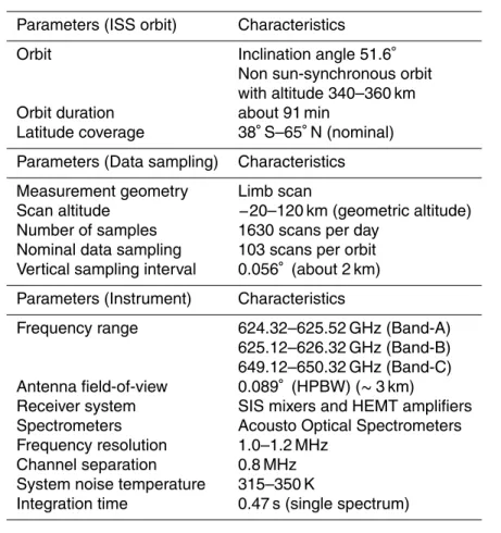
the instrument and its performance are available in JEM/SMILES Mission Plan (2002). A summary of the specifications of SMILES is shown in Table 1. The SMILES instru-ment employed 4 K submillimeter-wave superconductive heterodyne receivers, and ob-tained spectra with unprecedented low noise, which is one order of magnitude better performance than previous microwave/sub-millimeter limb instruments in space.
15
These unique observations gave us new products, such as the diurnal variation of short-lived radical species in the stratosphere and mesosphere. SMILES observations provided vertical abundance profiles of O3, H35Cl, H37Cl, ClO, HOCl, HO2, H2O2, BrO, HNO3, O3isotopologues, CH3CN, H2O, as well as ice clouds, winds, and temperature from the stratosphere to the lower thermosphere.
20
The JEM/SMILES mission is a joint project of the National Institute of Information and Communications Technology (NICT) and the Japan Aerospace Exploration Agency (JAXA). In this paper, we assess the O3vertical profiles for the SMILES NICT Level-2 (L2) version 2.1.5 product, which used the version 007 calibrated Level-1b (L1b) spec-tra. Hereafter, we denote SMILES NICT L2 products version 2.1.5 as “SMILES”. We
25
AMTD
6, 2643–2720, 2013SMILES O3 validation
(NICT L2-v215)
Y. Kasai et al.
Title Page
Abstract Introduction
Conclusions References
Tables Figures
◭ ◮
◭ ◮
Back Close
Full Screen / Esc
Printer-friendly Version
Interactive Discussion
Discussion
P
a
per
|
Dis
cussion
P
a
per
|
Discussion
P
a
per
|
Discussio
n
P
a
per
|
The structure of the paper is as follows: SMILES O3 observation characteristics are shown in Sect. 2 which includes, the instrumental configuration and observation sam-pling pattern (Sect. 2.1), the retrieval algorithm (Sect. 2.2), and O3 observation char-acteristics from error analysis (Sect. 2.3). The internal SMILES comparisons, Sect. 3, is consists of two parts. First, in Sect 3.1, we present the comparison of three different
5
instrumental receiver configurations for the same O3 625.371 GHz transition spectral measurements to evaluate the instrumental uncertainty and characteristics. Second, in Sect. 3.2, we describe the comparison of two different retrieval algorithms applied
to the same SMILES 625.371 GHz O3 spectra. The external comparisons are shown
in Sect. 4. The comparison with ozonesonde measurements is provided in Sect. 4.2,
10
and Sect. 4.3 gives the comparison with satellite observations from ENVISAT/MIPAS, SCISAT/ACE-FTS, Odin/OSIRIS, Odin/SMR, Aura/MLS, and Sect. 4.4 shows the com-parison with balloon born measurement TELIS. These observations performed at var-ious different local times. Finally, an example of the diurnal variation of O3is shown in Sect. 5 with SMILES observation samplings from the ISS.
15
2 SMILES O3characteristics: observation, retrieval, and error
2.1 SMILES O3observation
We performed the validation analysis for the main O3(16O16O16O) observation at the transition frequency 625.371 GHz for (J,Ka,Kc)=(15, 6, 10)−(15, 5, 11), while SMILES observed other kinds of O3, such as O3isotopologues (asym-17-O3, sym-18-O3,
sym-20
17-O3, sym-18-O3) and several vibrationally-excited state O3transitions. Details of the SMILES O3observations are shown in Kasai et al. (2006).
SMILES has three different instrument (receiver) configurations for observing the 625.371 GHz O3 transition. One of the purposes for this was to evaluate the char-acteristics of the receiver systems by comparing results from the same 625.371 GHz
25
O3 observation. The targeted 625.371 GHz O3 transition is allocated in two frequency
AMTD
6, 2643–2720, 2013SMILES O3 validation
(NICT L2-v215)
Y. Kasai et al.
Title Page
Abstract Introduction
Conclusions References
Tables Figures
◭ ◮
◭ ◮
Back Close
Full Screen / Esc
Printer-friendly Version
Interactive Discussion
Discussion
P
a
per
|
Dis
cussion
P
a
per
|
Discussion
P
a
per
|
Discussio
n
P
a
per
|
regions Band-A (624.32–625.52 GHz) and Band-B (625.12–626.32 GHz). SMILES em-ployed two Acousto Optical Spectrometers (AOSs) with a bandwidth of 1.2 GHz, which are denoted as AOS1 and AOS2 in this paper. The combinations of the two frequency bands (A and B) and two spectrometers (AOS1 and AOS2) resulted in three different instrumental setups for the 625.371 GHzO3 measurements; that is, (1) Band-A with
5
AOS1, (2) Band-A with AOS2, and (3) Band-B with AOS2. The Band-B observation was always performed with the spectrometer AOS2. During each measurement, two out of the three SMILES frequency bands were observed simultaneously, i.e. A+B, C+B, and C+A.
Figure 1 shows the number of SMILES O3observations for each day of the mission
10
by 5◦ latitude bins. For several specific periods, the ISS rotated 180◦ around its yaw axis and thus the observation latitude range was shifted to southern high latitudes. Relatively high sampling density is shown at both ends of the latitudinal range where the orbit changes from the ascending to descending phase. In each orbit there was a period when the ISS solar array wing (solar paddle) disturbed the observation
line-15
of-sight (LOS) of SMILES, which rendered the observed data useless. This decreases the sampling density as shown by the dark blue X shapes in Fig. 1. The decrease in number of measurement was typically 4.5–8.4 % (of the daily 1630 scans) during Oc-tober 2009–April 2010, however in December 2009 when the measurement decreased by 48 %.
20
2.2 SMILES O3retrieval procedure
Vertical profiles of the O3 volume mixing ratio (VMR) for SMILES v2.1.5 are derived from the L1b version 007 calibrated spectra. A summary of the SMILES L1b products and associated L2 products are shown in Table 2.
The retrieval algorithm is based on the least-squares method with a priori constraint
25
AMTD
6, 2643–2720, 2013SMILES O3 validation
(NICT L2-v215)
Y. Kasai et al.
Title Page
Abstract Introduction
Conclusions References
Tables Figures
◭ ◮
◭ ◮
Back Close
Full Screen / Esc
Printer-friendly Version
Interactive Discussion
Discussion
P
a
per
|
Dis
cussion
P
a
per
|
Discussion
P
a
per
|
Discussio
n
P
a
per
|
functions of SMILES. For submillimeter-wave limb observations from space, continuum absorptions due to H2O and dry-air become one of the dominant opacity sources in the lower stratosphere. The SMILES continua absorptions model was made based on a model described in Pardo et al. (2001). The dry air continuum absorption coefficient was increased by a factor of 20 % from the original formula, in order to give a better
5
agreement with the theoretical models (e.g. Boissoles et al., 2003) in the SMILES frequency range.
The version 2.X.X series of the NICT L2 processing focuses on analysis in the
mid-dle stratosphere and the mesosphere. We used the O3 spectra with only 570 MHz
bandwidth, in the frequency region of 625.042–625.612 GHz, instead of using the full
10
1.2 GHz bandwidth of the AOS in order to obtain a better fit of the spectral baseline and to stabilize the retrieval procedure. Such a reduction in the spectral bandwidth results in the removal of information coming from the wing of the O3line, and thus it degrades the sensitivity to O3at lower altitudes such as the upper troposphere.
The first of all, we performed the correction of the tangent height information before
15
retrieving all other jacobians such as O3 profiles. The LOS elevation angles (i.e. tan-gent heights of the limb measurements) were corrected for each spectrum by deriving the information from the pressure-induced spectral linewidth of the O3line. The perfor-mance of LOS elevation angle retrieval using the O3 transition is discussed in Baron et al. (2011).
20
Second, the O3 profiles were retrieved including following parameters as additional variables: temperature, HCl, HNO3, HOCl, H2O, and a linear baseline of the spectrum. An offset for the LOS elevation angle was again set as a variable at this step in order to obtain a better fit on the measurement. We used a priori information for O3, H2O, temperature, and pressure from the analysis of the Goddard Earth Observing System
25
Model version 5.2 (GEOS-5.2) (Rienecker et al., 2008). The inversion grid is 3 and 4 km-steps for 16.5–61.5 km, 65–81 km, respectively, with additional 86, 92, and 100 km levels.
AMTD
6, 2643–2720, 2013SMILES O3 validation
(NICT L2-v215)
Y. Kasai et al.
Title Page
Abstract Introduction
Conclusions References
Tables Figures
◭ ◮
◭ ◮
Back Close
Full Screen / Esc
Printer-friendly Version
Interactive Discussion
Discussion
P
a
per
|
Dis
cussion
P
a
per
|
Discussion
P
a
per
|
Discussio
n
P
a
per
|
Figure 2 shows an example of the SMILES O3retrieval. The version 2.1.5 of NICT L2 processing uses the SMILES measurements which tangent heights are within 15– 110 km, and three of them are shown in the plot as examples. The retrieved O3profile from this single scan measurement is shown in the middle panel with information on the 1-σretrieval error and vertical resolution. Averaging kernels (right panel on Fig. 2)
5
describe the sensitivity of the retrieved O3 abundance to the true state. Their vertical spread is used as an indication of the vertical resolution of the retrievals. It is 3–4 km, 4–6 km, and 6–10 km at 50–0.2 hPa, 0.2–0.02 hPa and 0.02–0.001 hPa, respectively.
The measurement response is the sum of the elements of each averaging kernel row, where low values indicate high contributions from the a priori state to the retrieved
infor-10
mation. We assessed the quality of retrieval by using the following quantities: goodness of the fit based on the chi-square statisticsχ2after the retrieval, averaging kernels, and
the measurement response, m. The χ2 used in the SMILES NICT processing is the
summation of the squared and variance weighted residuals in the measurement space and the null space after they are normalized by the numbers of measurements and
re-15
trieval parameters (see Eq. 2 given by Baron et al., 2011). A typicalχ2of the SMILES v2.1.5 O3product is 0.6–0.8 being smaller than unity is because of the overestimation of the measurement noise (Baron et al., 2011). Hereafter, we considerχ2≤0.8 as the data selection threshold to remove bad-fitted scans. The condition formis also set to be larger than 0.8. This gives the sensitivity range of the SMILES O3from a single scan
20
as 100–0.001 hPa (∼16–90 km).
2.3 Error analysis of SMILES O3vertical profile
Two components are important to explaining the SMILES systematic error: one is the uncertainty in the forward model parameterization, and the other is the uncertainty of the calibration of L1b spectra. We estimated such systematic errors for the single scan
25
AMTD
6, 2643–2720, 2013SMILES O3 validation
(NICT L2-v215)
Y. Kasai et al.
Title Page
Abstract Introduction
Conclusions References
Tables Figures
◭ ◮
◭ ◮
Back Close
Full Screen / Esc
Printer-friendly Version
Interactive Discussion
Discussion
P
a
per
|
Dis
cussion
P
a
per
|
Discussion
P
a
per
|
Discussio
n
P
a
per
|
the other ones with the original forward model used in the SMILES v2.1.5 processing. The measurements were simulated using the Band-B characteristics with five randomly selected O3reference profiles from the GEOS-5.2 data for the equatorial daytime con-ditions.
The error sources and their perturbation parameters are summarized in Table 3. The
5
uncertainty in the spectroscopic parameters includes the target O3line and also other species. The uncertainty related to the SMILES instrument functions is given by the SMILES instrument team, for example, Ochiai et al. (2012), Mizobuchi et al. (2012) and Sato et al. (2012).
The NICT v2.1.5 processing uses simplified instrumental functions regarding to the
10
antenna field-of-view (FOV) drift during data integration of one spectrum at each tan-gent point (0.47 s) and the effect from the image side-band signal. The SMILES an-tenna FOV drifts about a half of its half-power-beam-widths (HPBW) beam size during 0.47 s; however, the forward model assumes an antenna response pattern with an in-stantaneous single-FOV pointing at each tangent height for the observed spectra. This
15
makes an underestimation of the HPBW of the effective antenna response pattern. For the image side-band signal treatment, the NICT v2.1.5 processing did not take this into account because its impact was thought to be negligible for the main target vertical ranges.
The error from the uncertainty of the registered tangent height information is not
20
included as an explicit error source in the presented error analysis because these are retrieved in the processing. However, since the O3 retrieval was carried out based on this retrieved tangent height information, errors on the O3retrieval can be introduced if any errors exist in the tangent height retrievals. Such an error propagation is considered in our error analysis simulations.
25
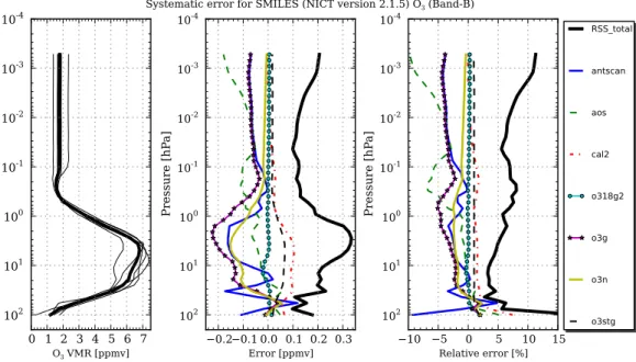
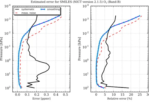
Figure 3 shows the estimated systematic errors for the NICT v2.1.5 O3 retrieval. The same analysis for the Band-A configuration was performed and we got almost the same results as Band-B. Total systematic error, labelled as “RSS total” in Fig. 3, was calculated as a root-sum-square (rss) of all the considered error factors. The negative
AMTD
6, 2643–2720, 2013SMILES O3 validation
(NICT L2-v215)
Y. Kasai et al.
Title Page
Abstract Introduction
Conclusions References
Tables Figures
◭ ◮
◭ ◮
Back Close
Full Screen / Esc
Printer-friendly Version
Interactive Discussion
Discussion
P
a
per
|
Dis
cussion
P
a
per
|
Discussion
P
a
per
|
Discussio
n
P
a
per
|
sign means that the v2.1.5 processing underestimated O3profile. On the plot, only the error sources with an impact larger than 5 % of the total rss error are shown (which confirms that the image side-band signal can be neglected in the stratosphere). The largest error source is the air-pressure broadening coefficient (“o3g”) followed by its temperature dependence (“o3n”) and the antenna FOV drift treatment (“antscan”). The
5
uncertainty on the air-pressure broadening coefficient can bias the O3retrieval by more than 5 % in the stratosphere. The non-linearity in the gain correction (“cal2”) was esti-mated by assuming 20 % uncertainty in the gain compression factor, yielding an error of 0.1 ppmv (∼1.8 %) in the stratosphere. The total systematic error was estimated to be about 3–8 % in the stratosphere with this being 3.8 % at the peak of the O3profile.
10
For the mesosphere (pressure ≤∼0.2 hPa), the uncertainty in the AOS response
function becomes one of the dominant sources of the systematic error (5–10 %). This
is because the O3linewidth becomes comparable or narrower than the FWHM of the
AOS response function. For comparison, the measurement noise (O3error due to sta-tistical noises of the SMILES measurement) and the smoothing error (error introduced
15
in the inversion analysis) from a single scan are also shown in the Fig. 4. These two errors can be considered as the random error of the O3profile, and are much smaller than the systematic error in the stratosphere. The measurement noise error is kept very low compared to the systematic errors, even smaller than 1 % of the retrieved O3 profile, at 50–1 hPa. This emphasizes the importance of understanding the systematic
20
AMTD
6, 2643–2720, 2013SMILES O3 validation
(NICT L2-v215)
Y. Kasai et al.
Title Page
Abstract Introduction
Conclusions References
Tables Figures
◭ ◮
◭ ◮
Back Close
Full Screen / Esc
Printer-friendly Version
Interactive Discussion
Discussion
P
a
per
|
Dis
cussion
P
a
per
|
Discussion
P
a
per
|
Discussio
n
P
a
per
|
3 Internal comparisons within various SMILES O3products
3.1 Comparison between two different observational configurations
As described in Sect. 2.1, SMILES has three configurations for observing the O3
625.371 GHz transition. The observation configuration set of Band-A (AOS1)+
Band-B (AOS2) (denoted as A+B mode hereafter) measured the same spectrum within the
5
same air mass with nearly same instrumental front-end characteristics (antenna char-acteristics, antenna scanning pattern, the optical characteristics). Comparing the O3 profiles retrieved from the two bands under the A+B configuration helps in assessing the difference of the instrumental characteristics of each receiver and the spectrome-ter, which are the most important instrumental characteristics for estimating the gain
10
calibration accuracy.
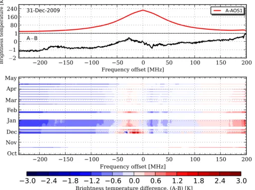
Figure 5 shows the difference between the calibrated radiances of the
Band-A (Band-AOS1) and Band-B (Band-AOS2) spectra during the SMILES observation period. The residual clearly shows the variations along the observation period as shown in the bot-tom panel of Fig. 5. The brightness temperature difference was small in October 2009
15
(daily average of the rms difference was as small as 0.3 K), and sharply increased in
December (average rms was ∼0.8 K). Such characteristics may be explained by the
change of the AOS operational configuration: the thermal control system of the AOS spectrometers was switched offat the end of October 2009 for a longer life-time. The gain calibration of the SMILES L1b radiance spectra version 007 uses the calibration
20
parameters based on the observations performed early October 2009. It is likely that the change in the AOS characteristics before and after thermal control was switched off introduced a significant change in the parameters for the non-linearity gain cali-bration. This issue will be investigated future using the next version of the L1b data inwhich it is planned to implement non-linearity gain calibration parameters evaluated
25
with considering the different conditions of the AOS thermal control.
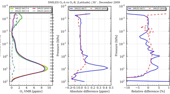
Figure 6 shows the comparison between O3profiles observed with Band-A (AOS1) and Band-B (AOS2) using the A+B measurements. The data are from the latitudinal
AMTD
6, 2643–2720, 2013SMILES O3 validation
(NICT L2-v215)
Y. Kasai et al.
Title Page
Abstract Introduction
Conclusions References
Tables Figures
◭ ◮
◭ ◮
Back Close
Full Screen / Esc
Printer-friendly Version
Interactive Discussion
Discussion
P
a
per
|
Dis
cussion
P
a
per
|
Discussion
P
a
per
|
Discussio
n
P
a
per
|
range 30◦S–30◦N in December 2009. The center and right panels show the mean of the absolute and relative differences, respectively. Note the relative difference is defined as the ratio to the reference O3profile, which is the mean of two compared profiles. In this subsection we focus to the result for SMILES(NICT) profiles, and the results for SMILES(JAXA) will be discussed in Sect. 3.2.
5
The O3 VMRs of SMILES(NICT) Band-A are significantly (∼0.4 ppmv, or 5 % at
8.3 hPa level) larger than those of Band-B. In the error analysis presented in Sect. 2.3, we do not find any error source which can reproduce such significant differences be-tween Band-A and Band-B processing. This indicates that there are unimplemented error sources (or imperfect modeling of gain calibration uncertainty) in our analysis
10
and/or the considered perturbation was underestimated. We consider that the actual difference between Band-A and B O3profiles is most likely due to the gain calibration uncertainty of the L1b spectrum being amplified by the LOS elevation angles (tangent heights) correction procedure of SMILES(NICT) processing. The LOS elevation angles retrieved from the coincident Band-A and B measurements differ by ∼0.006◦ (300 m)
15
for tangent heights around 30–35 km. This 300 m error propagates in the O3 VMR
retrieval which uses again the L1b spectrum with gain calibration errors, and finally results in such significant VMR differences between the O3 profiles from Band-A and Band-B. This issue will be further discussed in Sect. 3.2.2 by comparing the Band A–B discrepancies of NICT and JAXA L2 processings.
20
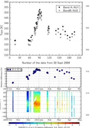
The seasonal and latitudinal changes in the differences between SMILES(NICT) v2.1.5 O3profiles from Band-A and B are shown in Fig. 7. The A–B difference in the O3 profiles at 8.3 hPa is very small in October 2009. This is consistent with the difference in the L1b spectral radiance shown in Fig. 5. Some of the seasonal behavior of the O3 Band-A and B difference, such as a large change during December 2009, follows
25
AMTD
6, 2643–2720, 2013SMILES O3 validation
(NICT L2-v215)
Y. Kasai et al.
Title Page
Abstract Introduction
Conclusions References
Tables Figures
◭ ◮
◭ ◮
Back Close
Full Screen / Esc
Printer-friendly Version
Interactive Discussion
Discussion
P
a
per
|
Dis
cussion
P
a
per
|
Discussion
P
a
per
|
Discussio
n
P
a
per
|
trend of the system noise temperature. Further investigations regarding to the sensitiv-ity of O3retrieval to the instrumental characteristics are now under way using the newly calibrated L1b spectra 008.
3.2 Comparison with JAXA-processed SMILES O3profiles
3.2.1 Major differences in the O3retrieval algorithms 5
We performed a comparison of the NICT-processed SMILES v2.1.5 O3 profiles with
those retrieved by the JAXA L2 processing version 2.0 (007-08-0300). These two L2 data products are denoted as SMILES(NICT) and SMILES(JAXA), respectively in this section.
Both L2 products are retrieved from the same version of the SMILES spectra (L1b
10
007), used the same principal retrieval algorithm (i.e. the least-squares method with regularization based on a priori constraints), and used the same instrumental functions in the forward model excepting the antenna FOV drift and image side-band signal treat-ments (as discussed in Sect. 2.3). The major differences in these processors which have possibility to give significant impacts on O3 retrieval results for SMILES(NICT)
15
and SMILES(JAXA) are as follow:
1. Forward model-radiative transfer:
– O3 spectroscopic parameters: two L2 processings use the almost same pa-rameters for theγ (2.31 MHz hPa−1) of the O3 line, but the temperature
de-pendence n of the γ is different. SMILES(NICT) and SMILES(JAXA) used
20
0.73 (based on the parameter used in the Aura/MLS data processing) and 0.78 (based on the HITRAN 2008 database, Rothman et al., 2009), respec-tively.
– Continuum model in the sub millimeter-wave region: SMILES(NICT) uses the continuum model based on the work by Pardo et al. (2001) with an empirical
25
AMTD
6, 2643–2720, 2013SMILES O3 validation
(NICT L2-v215)
Y. Kasai et al.
Title Page
Abstract Introduction
Conclusions References
Tables Figures
◭ ◮
◭ ◮
Back Close
Full Screen / Esc
Printer-friendly Version
Interactive Discussion
Discussion
P
a
per
|
Dis
cussion
P
a
per
|
Discussion
P
a
per
|
Discussio
n
P
a
per
|
scaling as described in Sect. 2.2, while SMILES(JAXA) uses the Liebe-93 model (Liebe et al., 1993) with a scaling factor of 1.34.
2. Forward model-instrumental function:
– Drift of SMILES antenna FOV: the SMILES(NICT) takes a single
instanta-neous FOV pointing at each tangent height, whereas the SMILES(JAXA)
5
uses a more realistic antenna pattern by convolving the drift of the antenna FOV during the data integration of a spectrum at one tangent height.
3. Retrieval setups:
– Inversion approach and the spectral bandwidth used in the retrieval: the SMILES(NICT) v2.1.5 processor is based on a sequential inversion approach
10
for each major retrieval parameter. It first retrieves the tangent height infor-mation and then O3 and temperature. Both retrieval steps for the tangent heights and O3VMRs employ a 570 MHz-bandwidth spectral region centered at 625.371 GHz. The SMILES(JAXA) processor uses the full spectral range of AOS bandwidth, 1.2 GHz, and retrieves all physical parameters
simultane-15
ously.
– Tangent height retrieval: SMILES(NICT) retrieves the LOS elevation angles for each tangent height of the limb scan measurement and corrects them prior to the O3 retrieval, while SMILES(JAXA) retrieves a single offset parameter for the LOS elevation angle.
20
– Temperature a priori and its retrieval: a priori temperature and pressure pro-files used in the SMILES(NICT) processor are based on the GEOS-5.2 anal-ysis and MSIS climatology data. In the SMILES(JAXA) processing they are based on the GEOS-5.2 and MLS version 2.2 data product and include the effect of migrating tides. Both the SMILES(NICT) and the SMILES(JAXA)
pro-25
AMTD
6, 2643–2720, 2013SMILES O3 validation
(NICT L2-v215)
Y. Kasai et al.
Title Page
Abstract Introduction
Conclusions References
Tables Figures
◭ ◮
◭ ◮
Back Close
Full Screen / Esc
Printer-friendly Version
Interactive Discussion
Discussion
P
a
per
|
Dis
cussion
P
a
per
|
Discussion
P
a
per
|
Discussio
n
P
a
per
|
constraint above 40 km which does not allow noticeable deviations of the re-trieval from the a priori profile at these high altitudes, and no retrieved infor-mation comes for the temperature profile. Thus the temperature inforinfor-mation for SMILES(JAXA) becomes identical to that of the a priori profile at those high altitudes. However, the SMILES(NICT) processor retrieves the
temper-5
ature profile simultaneously with O3VMR profile.
– Hydrostatic equilibrium condition: SMILES(JAXA) processor uses the hydro-static equilibrium condition to correct the pressure profile every time after the temperature profile is retrieved. In contrast, the SMILES(NICT) processing does not employ the hydrostatic equilibrium condition. The reason for this
10
is to avoid propagation of errors originating in the temperature retrieval. As shown in Baron et al. (2011), retrieving the tangent heights independently and representing the retrieved VMR profiles on pressure levels significantly reduced the impacts of the pressure errors on the O3retrieval.
– A priori profiles and vertical correlations for O3: SMILES(NICT) uses a priori
15
information based on the GEOS-5.2 analysis with a 3 km correlation length in the vertical grid, while SMILES(JAXA) uses data from the monthly, latitudi-nally, and day–night separately averaged MLS v2.2 product with nearly-zero correlations.
3.2.2 Comparison of the SMILES(NICT) and the SMILES(JAXA) O3profiles 20
As shown in Fig. 6, both SMILES(NICT) and SMILES(JAXA) O3 profiles have
dis-crepancies between those retrieved from the coincident measurements of Band-A
and Band-B. The A–B discrepancy in the SMILES(JAXA) O3 is smaller than that in
SMILES(NICT), but still not negligible.
In the differences found between SMILES(NICT) and SMILES(JAXA) profiles, the
25
negative values below the O3 peak (∼10 hPa) and the positive values above indi-cate a significant error due to a bias from the tangent height retrieval. When the LOS
AMTD
6, 2643–2720, 2013SMILES O3 validation
(NICT L2-v215)
Y. Kasai et al.
Title Page
Abstract Introduction
Conclusions References
Tables Figures
◭ ◮
◭ ◮
Back Close
Full Screen / Esc
Printer-friendly Version
Interactive Discussion
Discussion
P
a
per
|
Dis
cussion
P
a
per
|
Discussion
P
a
per
|
Discussio
n
P
a
per
|
elevation angle correction of SMILES(NICT) retrieval is turned offbefore O3 retrieval,
the Band A–B discrepancy on SMILES(NICT) O3was same as that of SMILES(JAXA)
as shown in Fig. 6. This means that the SMILES(NICT) O3retrieval algorithm enhanced the error on O3retrieval (at maximum 5 % in the stratospheric region) through its way of applying the tangent height correction. The root cause of such an error-amplification
5
is considered to be the uncertainty in the gain calibration. This Band A–B difference is expected to be reduced in the next version of SMILES(NICT) L2 product by using the improved gain calibration L1b spectra (version 008).
We performed the SMILES(NICT)–SMILES(JAXA) comparisons for three instrumen-tal subsets: (1) O3observed in A with AOS1 (2) A with AOS2, and (3)
Band-10
B with AOS2, in order to examine the effects of the different radiometer bands and different spectrometers, separately.
Figure 8 shows the mean absolute and relative differences in absolute and relative
amplitudes between the SMILES(NICT) and SMILES(JAXA) O3 profiles for the three
instrumental configurations. The data were collected from the March 2010 observations
15
at the equatorial region (30◦S–30◦N). The number of scans used for the comparisons was∼2000, 5200, and∼7900 for the cases (1), (2), and (3), respectively.
The overall trends in the differences between the SMILES(NICT) and SMILES(JAXA) O3products were the same for three instrumental subsets. As shown in Fig. 3, the dif-ference at the O3maximum is sensitive to the differences of the antenna drifting model
20
and the pressure broadening parameter. The systematic bias between 2–0.01 hPa, where SMILES(NICT) shows smaller VMRs than those of SMILES(JAXA), is quite likely explained to be due to the difference in the tangent height corrections of both retrieval algorithms. The oscillation in the difference in the middle/upper mesosphere is considered to be due to several reasons including the difference in the temperature
25
AMTD
6, 2643–2720, 2013SMILES O3 validation
(NICT L2-v215)
Y. Kasai et al.
Title Page
Abstract Introduction
Conclusions References
Tables Figures
◭ ◮
◭ ◮
Back Close
Full Screen / Esc
Printer-friendly Version
Interactive Discussion
Discussion
P
a
per
|
Dis
cussion
P
a
per
|
Discussion
P
a
per
|
Discussio
n
P
a
per
|
Looking into the details of band and AOS dependencies of the O3 differences in Fig. 8, the largest difference could be found for the case of Band-A with AOS2 (i.e. when SMILES observed O3 with the Band C+A configuration). The relative diff er-ence is 12 % at 8.3 hPa. When Band-A is used with AOS1 (A+B configuration), the difference became slightly smaller (10 %) at 10 hPa than that of the C+A case. The
5
Band-B (always observed with the AOS2) O3 has the best agreement between the
SMILES(NICT) and SMILES(JAXA) products around 10 hPa, although it still differs by
∼5 %. Considering that the SMILES(NICT)–SMILES(JAXA) difference is strongly af-fected by the gain calibration errors, our comparisons suggest that the gain calibration accuracy seems to be better for Band-B. A small impact of the AOS is found for the
10
Band-A retrievals in the stratosphere.
We investigated the impact of the different approaches for the tangent height correction and the hydrostatic equilibrium constraint between SMILES(NICT) and SMILES(JAXA). Figure 9 shows the change in the SMILES(NICT)–SMILES(JAXA) dif-ference when we turned offthe tangent height correction before the O3 retrieval, and
15
also including the hydrostatic equilibrium condition in the SMILES(NICT) processing. Without the tangent height correction, the altitude where the maximum SMILES(NICT)– SMILES(JAXA) difference exists becomes slightly higher at ∼3–5 hPa where corre-sponds to the steepest slope in O3 VMR profile. The difference then goes to zero around the 1 hPa level, and at the altitudes higher than 0.5 hPa the new SMILES(NICT)
20
profile shows larger O3 VMRs than SMILES(JAXA) which is the opposite trend to that shown in the original SMILES(NICT)–SMILES(JAXA) compositions. When we applied the hydrostatic equilibrium condition, the discrepancy between the SMILES(NICT) and
the SMILES(JAXA) O3 profiles increased in the mesosphere (pressures lower than
1 hPa). This demonstrates that the difference in the temperature profile amplifies the
25
difference in O3 retrieval through the application of the hydrostatic equilibrium: diff er-ences in the temperature profile induce differences in the pressure profile, and then propagate to the differences in O3 VMR. The SMILES(NICT) v2.1.5 processor does
AMTD
6, 2643–2720, 2013SMILES O3 validation
(NICT L2-v215)
Y. Kasai et al.
Title Page
Abstract Introduction
Conclusions References
Tables Figures
◭ ◮
◭ ◮
Back Close
Full Screen / Esc
Printer-friendly Version
Interactive Discussion
Discussion
P
a
per
|
Dis
cussion
P
a
per
|
Discussion
P
a
per
|
Discussio
n
P
a
per
|
not employ the hydrostatic equilibrium constraint in order to avoid such error amplifica-tions.
Finally, the seasonal and latitudinal changes in the SMILES(NICT)–SMILES(JAXA) difference are shown in Fig. 10. The top panel shows the seasonal evolution of the daily averaged differences at 8.3 hPa from the equatorial region. The SMILES(NICT)–
5
SMILES(JAXA) difference for the Band-B O3retrieval stayed relatively small compared to the Band-A products during the entire SMILES observation period. In the Sect. 3,
we noted that the Band-A and Band-B difference for the SMILES(NICT) product is
smaller when ISS rotated 180◦(Fig. 7). The latitudinal variation resembles the pattern of the previously shown inter-band difference band-A and Band-B that has a larger
10
discrepancy at the equatorial latitudes.
4 External comparisons
4.1 Methodology of comparisons
The comparison of the two O3profile data sets were performed by finding pairs of the coincident measurements, using a methodology which is based on the works by Dupuy
15
et al. (2009), von Clarmann (2006), and Chauhan et al. (2009). We set a horizontal dis-tance of within 300 km on the measurement location as a criteria for selecting a pair of coincident measurements between SMILES and other satellite/balloon-borne instru-ments. A 3-h threshold for the measurement time difference was also applied except for the comparisons with the ACE-FTS and ozonesonde measurements for which used
20
a 12-h criteria because of their more sparse measurements.
The data quality selection criteria for the SMILES data set was as follows.
– the measurement response (m)≥0.8
AMTD
6, 2643–2720, 2013SMILES O3 validation
(NICT L2-v215)
Y. Kasai et al.
Title Page
Abstract Introduction
Conclusions References
Tables Figures
◭ ◮
◭ ◮
Back Close
Full Screen / Esc
Printer-friendly Version
Interactive Discussion
Discussion
P
a
per
|
Dis
cussion
P
a
per
|
Discussion
P
a
per
|
Discussio
n
P
a
per
|
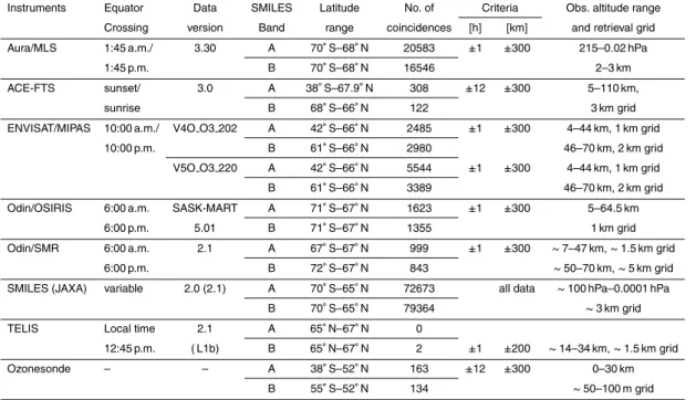
We also applied a certain data quality selection for the compared instruments based on the recommendation from each data processing team. A summary of the coincidences for each comparison dataset is given in Table 4.
The ozonesonde measurements have a vertical resolution about 50–100 m. The ver-tical resolutions for the satellite measurements are about 1.0–2.0 km, 2.5–6.0 km, 2.7–
5
3 km, 3–4 km for OSIRIS, MIPAS, SMR (J ´egou et al., 2008), MLS (Froidevaux et al., 2008), and ACE-FTS, respectively. We applied a vertically-smoothing triangle function as shown in Eq. (1), using the width of SMILES averaging kernel, for the ozonesonde and Odin/OSIRIS datasets. Direct comparison are applied for MLS, SMR, MIPAS, and ACE-FTS since the vertical resolutions and sampling intervals are comparable with that
10
of SMILES.
This smoothing function is,
xsmooth(pi)=
Pni
j=1wj(p
raw
j −pi)·x
raw (prawj )
Pni
j=1wj(prawj −pi)
, (1)
wherexsmooth(pi) is the smoothed volume mixing ratio for the high-vertical resolution measurement at pressurepi,xrawis the original VMR of the high-resolution profile,wj
15
is the associated weight (function ofprawj −pi), andni is the number of grid points from the high-resolution measurements which exist within the SMILES vertical resolution-width layer centered atpi. Once the vertical resolutions are adjusted, we interpolated the O3VMR profiles into a reference vertical grid which was generated on a pressure coordinate with intervals of∼3 km. The interpolation of VMRs was done by using a
lin-20
ear interpolation with respect to the logarithm of the pressure levels.
The mean absolute difference,∆abs, at the pressure level,p, between the coincident O3profiles was calculated using
∆abs(p)= 1 N(p)
NX(p)
i=1
{xs(p)−xc(p)}, (2)
AMTD
6, 2643–2720, 2013SMILES O3 validation
(NICT L2-v215)
Y. Kasai et al.
Title Page
Abstract Introduction
Conclusions References
Tables Figures
◭ ◮
◭ ◮
Back Close
Full Screen / Esc
Printer-friendly Version
Interactive Discussion
Discussion
P
a
per
|
Dis
cussion
P
a
per
|
Discussion
P
a
per
|
Discussio
n
P
a
per
|
whereN(p) is the number of coincidences atp, andxs(p) andxc(p) are the VMRs at p for SMILES and comparison instrument, respectively. The mean relative difference in percent was calculated by using the mean of two O3profiles as a reference,
∆rel(p)= 1 N(p)
NX(p)
i=1
xs(p)−xc(p)
x(p) ×100 (3)
where the reference (x(p)) is
5
x(p)=1
2(xs(p)+xc(p)) (4)
except for the comparison with ozonesonde. The reference for the ozonesonde com-parison was set as equal to the ozonesonde measurement, i.e.x=xsonde. This is be-cause we consider that below 30 km the ozonesonde measurement technique is more reliable than that of SMILES (or any satellite-based remote sensing).
10
4.2 Ozonesonde
An ozonesonde is a balloon-borne instrument measuring the atmosphere in situ from the ground to ∼35 km, where the balloon bursts. They are launched from each ozonesonde station about once a week and measure the profile of O3, total pressure, temperature, and humidity. The vertical resolution of an ozonesonde profile is about
15
50–100 m.
We used the ozonesonde data available from the World Ozone and Ultraviolet Data Center (WOUDC) (http://www.woudc.org/) and the Southern Hemisphere Additional Ozonesondes (SHADOZ) project (http://croc.gsfc.nasa.gov/shadoz/) (Thompson et al., 2003) for the dates from 12 October 2009 to 21 April 2010. We used the data from three
20
AMTD
6, 2643–2720, 2013SMILES O3 validation
(NICT L2-v215)
Y. Kasai et al.
Title Page
Abstract Introduction
Conclusions References
Tables Figures
◭ ◮
◭ ◮
Back Close
Full Screen / Esc
Printer-friendly Version
Interactive Discussion
Discussion
P
a
per
|
Dis
cussion
P
a
per
|
Discussion
P
a
per
|
Discussio
n
P
a
per
|
the same principle, which is to measure O3by using an electrochemical reaction cell containing a cathode (made of platinum) and an anode (made of platinum, silver or activated carbon) in a solution of potassium iodide (KI) (Kerr et al., 1994). According to Harris et al. (2002), the precisions of the three ozonesonde types are within±3 %, while systematic biases compared to other O3 sensing techniques are smaller than
5
±5 % between the tropopause and ∼28 km. Above 28 km, precision depends on the
type of ozonesonde. For example, the bias is−15 % at 30 km for the BM ozonesonde
and ±5 % for the ECC one. In addition, the precision for the ECC ozonesonde
de-pends on the manufacturer and the concentration of the solution of KI. For example, an ozonesonde with 1.0 % KI solution and a full buffer has a 5 % larger O3 VMR than
10
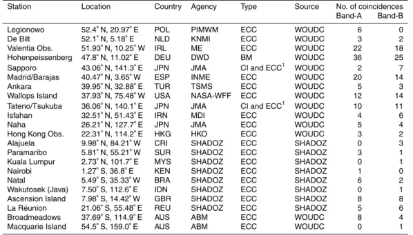
that with 0.5 % KI and a half buffer, and has a 10 % larger one than that with 2.0 % KI and no buffer (Smit et al., 2007). With the criteria of±12 h and±300 km, 159 and 133 coincidences were found for the comparison between SMILES Band-A and Band-B, as shown in Table 4. The ozonesonde stations where the coincidences were found are listed in Table 5 and plotted in Fig. 11.
15
The results are shown in Fig. 12. Two SMILES observation bands were treated sep-arately. The plot shows−7 to+8 % relative differences (−0.3–+0.5 ppmv in absolute
differences) between SMILES and ozonesondes in the pressure range between 40–
8 hPa (∼22 to 32 km). The difference is larger for Band-A compared to that of Band-B, which suggests the accuracy of SMILES O3 profile better for the Band-B product than
20
that for Band-A. The difference became larger with decreasing altitude. In the upper troposphere (e.g. pressures higher than 60 hPa), the SMILES O3 product VMRs were smaller than ozonesonde measurements by−20 %. According to the averaging kernels of the retrieval, it is supposed that the SMILES O3profiles still have sensitivity at pres-sure levels as high as 100 hPa (see Fig. 2). The accuracy of SMILES product at this
25
upper tropospheric region will be improved for the next version of NICT L2 processing.
AMTD
6, 2643–2720, 2013SMILES O3 validation
(NICT L2-v215)
Y. Kasai et al.
Title Page
Abstract Introduction
Conclusions References
Tables Figures
◭ ◮
◭ ◮
Back Close
Full Screen / Esc
Printer-friendly Version
Interactive Discussion
Discussion
P
a
per
|
Dis
cussion
P
a
per
|
Discussion
P
a
per
|
Discussio
n
P
a
per
|
4.3 Satellite-borne instruments
We performed the comparisons with Aura/MLS, SCISAT/ACE-FTS, ENVISAT/MIPAS,
Odin/OSIRIS, and Odin/SMR which observe O3 at various local times as shown in
Table 4.
4.3.1 Aura/MLS
5
The Aura satellite was launched on 15 July 2004 into a sun-synchronous orbit at 705 km altitude, with an ascending equator crossing time of 13:45 (Schoeberl et al., 2006). Its orbit is near-polar with a 98◦ inclination, and the daily Microwave Limb Sounder (MLS) measurements cover the latitudinal range from about 82◦S to 82◦N. MLS measures temperature and trace gas profiles (O3, H2O, HNO3, HCl, etc.) using thermal
emis-10
sion data (day and night scans) from the upper troposphere to the mesosphere. MLS performs each limb scan and related calibration in 25 s, and obtains∼3500 vertical profiles a day (Waters et al., 2006). The MLS data processing algorithms are based on the optimal estimation method, as explained by Livesey et al. (2006). MLS uses spec-tral bands centered near 118, 190, 240, and 640 GHz, as well as 2.3 THz, and obtains
15
standard Level 2 O3profiles from the 240 GHz spectral region (Livesey et al., 2006). The altitude range of a retrieved MLS O3 profile for version 3.3 (hereafter v3.3) is represented on a pressure grid encompassing 37 levels, equally-spaced on a log scale from 1000 to 1 hPa (e.g. 1000, 825, 681, 562, 464, 383, 316, 261, 215, 178, 147, 121, and 100 hPa for the first 13 levels), and including 18 levels (on a grid coarser by a factor
20
of two) above 1 hPa (Livesey et al., 2011).
We used the MLS v3.3 O3 product for the comparisons. Several MLS v2.2
val-idation studies have been published, e.g. Froidevaux et al. (2008); Dupuy et al. (2009); Chauhan et al. (2009); Jiang et al. (2007); Livesey et al. (2008). Accord-ing to Froidevaux et al. (2008), MLS v2.2 data exhibit differences of about 5–8 %
25
AMTD
6, 2643–2720, 2013SMILES O3 validation
(NICT L2-v215)
Y. Kasai et al.
Title Page
Abstract Introduction
Conclusions References
Tables Figures
◭ ◮
◭ ◮
Back Close
Full Screen / Esc
Printer-friendly Version
Interactive Discussion
Discussion
P
a
per
|
Dis
cussion
P
a
per
|
Discussion
P
a
per
|
Discussio
n
P
a
per
|
et al. (2009), a comparison between MLS v2.2 and the ACE-FTS version 2.2 O3
up-dated product shows 0 to 10 % difference between 12 and 43 km (∼2 hPa) and 10 to 25 % difference between 43 and 60 km. Validation of MLS v3.3 data is currently in progress but shows very small (1 to 2 %) differences versus the MLS v2.2 data for most of the stratosphere (Livesey et al., 2011). However, vertical profile O3oscillations
5
have become pronounced mainly at low latitudes in the upper troposphere and lower stratosphere; this issue is currently being studied further by the MLS team, with im-provements expected for the next data version. For the purposes of this work and the comparisons versus SMILES stratospheric O3data, the use of either MLS v2.2 or v3.3 data would result in very similar conclusions; the main difference has to do with the
10
finer (by a factor of two) vertical retrieval grid for the v3.3 data.
We performed the comparisons using MLS and SMILES profiles within±300 km and
±1 h, as mentioned in Sect. 4.1. We also used the MLS data screening
recommen-dations from the MLS team (see Livesey et al., 2011). We used the data that satisfy the conditions for each profile, such that “Status” field is even, “Quality”>0.6, and
15
“Convergence”<1.18. After data screening, we obtained 20 583 and 16 546 coinci-dences versus MLS profiles for the SMILES Band-A and band-B retrievals, respec-tively.
The results are shown in Fig. 13. The relative differences between SMILES and MLS are−11 to+3 % between 40 and 2 hPa (∼22–45 km). The Band-B profile is very close
20
to the MLS one (within 1 % difference) around 8–10 hPa (where the stratospheric peak in O3 VMR exists), while the SMILES Band-A product is larger than that of MLS by
+3 % (∼0.2 ppmv). Above 45 km, the relative differences are negative and worse than
−10 %. The vertical trend of the difference is roughly similar to that of the SMILES inter-nal comparison between SMILES(NICT) and SMILES(JAXA) (Fig. 8); but in detail one
25
can observe that the amplitude of the difference in the SMILES(NICT)-MLS compari-son decreases from−0.6 to −0.2 ppmv (from 1 to 0.1 hPa) while the SMILES(NICT)-SMILES(JAXA) comparison showed a constant−0.1 ppmv difference in that pressure range. In Sect. 3.2, we discussed that the difference of SMILES and SMILES(JAXA)
AMTD
6, 2643–2720, 2013SMILES O3 validation
(NICT L2-v215)
Y. Kasai et al.
Title Page
Abstract Introduction
Conclusions References
Tables Figures
◭ ◮
◭ ◮
Back Close
Full Screen / Esc
Printer-friendly Version
Interactive Discussion
Discussion
P
a
per
|
Dis
cussion
P
a
per
|
Discussion
P
a
per
|
Discussio
n
P
a
per
|
most likely comes from the impact of the different tangent height correction proce-dures. The result shown in Fig. 13 (which has a different vertical trend compared to the
SMILES(NICT) and SMILES(JAXA) comparison) means that the difference between
SMILES(NICT) and MLS data at higher altitudes is not solely due to the tangent height correction issue. One potential error source that could explain this difference is the
un-5
certainty in the modeling of the SMILES AOS response function. Indeed, if we compare MLS with the SMILES(NICT) Band-A data for the different AOSs, AOS1 and AOS2, in Fig. 14, we find that the SMILES(NICT)-MLS difference is not exactly the same at 1 hPa for AOS1 and AOS2 (−0.5 versus−0.65 ppmv).
The more significant difference shown at∼10 hPa in Fig. 14 is due to the effect of
10
uncertainty in the non-linearity gain calibration. The result is consistent with what we learned from the SMILES(NICT)–SMILES(JAXA) comparison shown in Fig. 8, that is
the SMILES O3 profile obtained with Band-A AOS2 tends to have larger VMR at 10–
8 hPa compared to that obtained with Band-A AOS1. Note that the differences between AOS1 and AOS2 are more moderate than those inferred in Fig. 8. This is because this
15
result is calculated with the coincident pairs from all latitudes while Fig. 8 was created using using only equatorial data, where larger differences exist between the AOSs (as shown in Fig. 10).
Improvements in the AOS response function parameterization are targeted for the next version of SMILES L1b calibration. It will be interesting to see how this changes
20
the comparisons versus MLS at high altitudes.
The seasonal and latitudinal variation of the relative difference at 8.3 hPa is shown in Fig. 15. The coincident pairs were divided into 2-days and 10◦-latitude pixels, and the median value of the relative differences were calculated for each pixel. Only the pixels where we had more than five coincident pairs are shown. Similarly to the results
25
AMTD
6, 2643–2720, 2013SMILES O3 validation
(NICT L2-v215)
Y. Kasai et al.
Title Page
Abstract Introduction
Conclusions References
Tables Figures
◭ ◮
◭ ◮
Back Close
Full Screen / Esc
Printer-friendly Version
Interactive Discussion
Discussion
P
a
per
|
Dis
cussion
P
a
per
|
Discussion
P
a
per
|
Discussio
n
P
a
per
|
dependence as those from Band-A. Some abnormal pixel differences are observed
for 60◦S in the middle of February, when SMILES observed high southern latitudes (69◦S).
4.3.2 SCISAT/ACE-FTS
The Canadian-led science mission, the Atmospheric Chemistry Experiment (ACE) on
5
the SCISAT satellite, was launched on 12 August 2003. The ACE satellite moves along an orbit inclined at 74◦ to the equator at 650 km altitude (Bernath et al., 2005). The ACE satellite has two instruments: the ACE Fourier Transform Spectrometer (ACE-FTS) (Bernath et al., 2005) and the Measurement of Aerosol Extinction in the Strato-sphere and TropoStrato-sphere Retrieved by Occultation (ACE-MAESTRO) (McElroy et al.,
10
2007). These observe the vertical profiles of O3 and a myriad of other trace gas con-stituents, temperature, and atmospheric extinction by aerosols.
The ACE-FTS measures the absorption of solar infrared radiation (750–4400 cm−1) with a high resolution of 0.02 cm−1. It observes sunrise and sunset about 30 times (15+15) per day and measures from cloud top to∼150 km with a vertical resolution of
15
about 3–4 km. The latitude range covered by ACE-FTS extends from 85◦S to 85◦N as given in Bernath et al. (2005).
The retrieval method is based on the Levenberg–Marquardt nonlinear least-squares method. Detailed information is given in Boone et al. (2005). The O3 vertical profiles are obtained from observed O3spectra in the frequency region of 829 cm−1, 923 cm−1,
20
1027–1168 cm−1, 2149 cm−1, and 2566–2673 cm−1. The retrieved data for O3 have a vertical profile range from ∼10 km to>90 km with 1-km spacing after interpolation (Boone et al., 2005).
We compared the SMILES v2.1.5 data (Band-A and -B) and the ACE-FTS version 3.0 data. The latest data version of ACE-FTS (version 3.0) is being validated
includ-25
ing comparisons with the previous version (version 2.2 O3) (Waymark et al., 2011).
AMTD
6, 2643–2720, 2013SMILES O3 validation
(NICT L2-v215)
Y. Kasai et al.
Title Page
Abstract Introduction
Conclusions References
Tables Figures
◭ ◮
◭ ◮
Back Close
Full Screen / Esc
Printer-friendly Version
Interactive Discussion
Discussion
P
a
per
|
Dis
cussion
P
a
per
|
Discussion
P
a
per
|
Discussio
n
P
a
per
|
ACE-FTS O3(version 3.0) profiles are improved compared to the v2.2 update profiles, with a 5–10 % decrease in VMR above 40 km.
Comparison results between ACE-FTS and SMILES (Band-A and Band-B) are shown in Fig. 16. Criteria are set as 300 km and ±12 h to obtain a sufficient number of coincidences. 308 and 122 coincidences were obtained for SMILES Band-A and
5
B, respectively. The SMILES O3 profiles have smaller VMRs at all heights except at 10 hPa for the Band-A data. There is a difference of−15 to−3 % for Band-B, and+1 % for Band-A at pressures of 40–1 hPa. The magnified of the difference is more signifi-cant than that of MLS. This is mainly due to a larger observation time difference (12 h) in the coincidence search.
10
4.3.3 ENVISAT/MIPAS
The Michelson Interferometer for Passive Atmospheric Sounding (MIPAS) is a mid-infrared emission spectrometer, which was a core payload of the European ENVIron-mental SATellite (ENVISAT) launched on 1 March 2002 (Fischer et al., 2008). ENVISAT moved at an altitude of 800 km and had a sun-synchronous orbit with 98.55◦inclination.
15
The descending equator crossing time was 10:00.
MIPAS observed five mid-infrared spectral bands within the frequency range 685 to 2410 cm−1(14.6–4.15 µm) with a resolution of 0.0625 cm−1(Cortesi et al., 2007). From 6 July 2002 to 26 March 2004, MIPAS scanned 17 tangent altitude from 6 to 68 km with 3–8 km resolution. The spectral resolution was 0.025 cm−1. At the end of March 2004,
20
excessive anomalies observed in the interferometer led to temporary discontinuation. However, it started again in a new operation mode from January 2005. In this opera-tional mode, MIPAS scanned at a reduced spectral resolution (0.0625 cm−1) and finer altitude grid. The latitudinal observation coverage was from 87◦S to 89◦N. In the latter mode, MIPAS had about 95 scans per orbit and conducted about 14.3 orbits per day
25
around the Earth. Thus, about 1360 vertical profiles were recorded in a day.
AMTD
6, 2643–2720, 2013SMILES O3 validation
(NICT L2-v215)
Y. Kasai et al.
Title Page
Abstract Introduction
Conclusions References
Tables Figures
◭ ◮
◭ ◮
Back Close
Full Screen / Esc
Printer-friendly Version
Interactive Discussion
Discussion
P
a
per
|
Dis
cussion
P
a
per
|
Discussion
P
a
per
|
Discussio
n
P
a
per
|
vertical profiles of temperature and six trace gases. However, several types of scientific data for trace gases exist that are not included in the ESA operational data. In this study, we used version V4O O3 202 of the MIPAS scientific data product, which is generated by Institut f ¨ur Meteorologie und Klimaforschung (IMK) at Karlsruhe Institute of technology (KIT) (von Clarmann et al., 2009). This data product was retrieved using
5
a Tikhonov-type regularization with a smoothing constraint (Steck and von Clarmann, 2001).
MIPAS IMK-IAA version V3O O3 7 data were compared with lidars, FTIR, balloon-borne instruments, and two satellite instruments (HALOE and POAM III) by Steck et al. (2007). According to that study, the mean relative differences for all instruments are
10
between±10 % above 18 km and 20 to 30 % below 18 km. In addition, the precision
is 5–10 % between ∼20 and 55 km, and the accuracy is 15–20 % between 20 and
55 km. The first version of the reduced spectral resolution L2 data product, version V4O O3 202, was compared with measurement data obtained by lidars, ozonsonde data, and satellite instruments during the Measurements of Humidity in the Atmosphere
15
and Validation Experiments (MOHAVE) 2009 campaign (Stiller et al., 2012). According to Stiller et al. (2012), the differences between the MIPAS O3 mean profile and mean profiles of most instruments were within±0.3 ppmv below 30 km. These MIPAS O3 pro-files have a positive bias up to+0.9 ppmv at 37 km. Between 50 and 60 km,−0.5 ppmv difference is found in the comparison between MIPAS profiles and ACE-FTS version
20
2.2 O3 profiles. However, the ACE-FTS version 2.2 O3 data have a positive bias from 45 to 60 km, as mentioned in Sect. 4.3.2. The positive MIPAS O3 bias around 37 km has been largely reduced in the V5O O3 220 version. The current status of the MIPAS data comparisons are reported (Laeng et al., 2012).
We performed the comparisons with ±300 km in a great circle and ±1 h, as
men-25
tioned in Sect. 4.1. With these criteria, 2485 and 2980 coincidences with MIPAS ver-sion V4O O3 202 profiles were found for Band-A and -B, respectively. The results are shown in Fig. 17. Comparison with MIPAS confirms the result of the SMILES valida-tion with MLS and ACE-FTS that SMILES ozone mixing ratios are low, except for the