Lat. Am. j. solids struct. vol.11 número14

Abstract

Exact solutions of buckling configurations and vibration response of post-buckled configurations of beams with non-classical bounda-ry conditions (e.g., elastically supported) are presented using the Euler-Bernoulli theory. The geometric nonlinearity arising from mid-plane stretching (i.e., the von Kármán nonlinear strain) is considered in the formulation. The nonlinear equations are re-duced to a single linear equation in terms of the transverse deflec-tion by eliminating the axial displacement and incorporating the nonlinearity and the applied load into a constant. The resulting critical buckling loads and their associated mode shapes are ob-tained by solving the linearized buckling problem analytically. The buckling configurations are determined in terms of the applied axial load and the transverse deflection. The first buckled shape is the only stable equilibrium position for all boundary conditions considered. Then the pseudo-dynamic response of buckled beams is also determined analytically. Natural frequency versus buckling load and natural frequency versus amplitudes of buckling configu-rations are plotted for various non-classical boundary conditions.

Keywords

Analytical solutions; buckling analysis; Euler-Bernoulli beam theo-ry; pseudo-dynamic analysis; von Kármán nonlinearity.

Buckling configurations and dynamic response of buckled

Euler-Bernoulli beams with non-classical supports

1 INTRODUCTION AND BACKGROUND

Beams are common structural elements in many engineering systems. Often beams are subjected to axial compressive loads, which cause them to buckle. Linear eigenvalue problems can be formu-lated to determine the buckling loads and buckling configurations for a variety of boundary con-ditions (see Reddy, 2004; 2007). In reality, beams subjected to axial loads develop axial internal forces that stretch the centroidal axis of the beam, resulting in the geometric nonlinearity that couples the axial displacement to the transverse displacement. Although onset of buckling does not imply total failure of the structure, the knowledge of the value of the load that initiates

buck-B. G. Sinira B. B. Özhanb J. N. Reddyc

a,b,c_{Department of Mechanical} Engi-neering Texas A&M University, College Station, TX 77843-3123, USA

a_{Department of Civil Eng. Celal Bayar} University, 45140 Manisa, Turkey

b_{Department of Mechanical} Engineer-ing; Applied Mathematics and Compu-tation Center, Celal Bayar University, 45140 Manisa, Turkey

c_{Corresponding author:} jnreddy@tamu.edu

ling is of value in the design of engineering structures.

The study of buckling of beams has received considerable attention in the last decade. Nayfeh and Emam (2008) and Emam and Nayfeh (2009) have obtained exact solutions for the buckling configurations of beams under classical boundary conditions, while including the von Kármán nonlinearity. Both of these studies claim to have carried out post-buckling analysis of beams, but they are flawed because the equation they have employed is not applicable for post-buckling analysis, as explained by Shen (2011). Furthermore, Sınır et al. (2010) showed numerically that the buckling configurations of clamped-pinned beams presented by Nayfeh and Emam (2008) and Emam and Nayfeh (2009) are incorrect, and Sınır (2010) presented the correct ones.

Although there exist analytical solutions of linear buckling of beam–columns using the Euler-Bernoulli and Timoshenko beam theories for both isotropic and laminated composite beams for classical boundary conditions (i.e., a combination of hinged, clamped, and free boundary condi-tions; see Reddy, 2004; 2007), to the best of the authors’ knowledge, analytical solutions of buck-ling as well as pseudo-dynamic response about buckled configurations of beam-columns consider-ing the von Kármán nonlinearity are not available for non-classical (e.g., edges with elastic sup-ports). In this study, we obtain analytical solutions for the buckling configurations and pseudo-dynamic response about buckled configurations of beams with a variety of non-classical boundary conditions using the Euler-Bernoulli beam theory. The critical buckling loads and their associated mode shapes are obtained analytically for buckled configurations first, and then pseudo-dynamic response about the buckled configurations is determined using a novel analytical method.

2 GOVERNING EQUATIONS

2.1 Displacements and Strains

The Euler-Bernoulli hypothesis of straight lines normal to the axis of the beam before defor-mation remain (a) straight after defordefor-mation, (b) inextensible, and (c) rotate as rigid lines to remain perpendicular the bent axis is satisfied by the following choice of the displacement field (see Reddy, 2004; 2007, and Figure 1)

1 ˆ1 3 ˆ3 ˆ ˆ

( )=u x z( , )e +u x z( , )e ºu x z_x( , )e_x +u x z_z( , )e_z

u x (1)

with

( , ) ( ) , ( , ) ( ),

x x z x

dw

u x z u x z u x z w x

dx

q q

= + = º - (2)

The simplified Green-Lagrange strain tensor [i.e., 2 2

1 1

(¶u ¶x) »0, (¶u ¶z) »0 ] is

ε (0) (1)

11 11 2 (0)

1 1

(1)

1

2 ˆ ˆ e e

,

, _{xx xx xx}

x

xx xx

z

d

du dw

dx dx dx

e e e e e

q

e e

= +

æ _ö÷

ç

+ ç_ç ÷_÷÷ =

è ø

= =

Figure1: Kinematics of the Euler–Bernoulli beam theory.

2.2 Equations of Motion

The equations of motion can be obtained using Hamilton’s principle (see Reddy, 2004; 2007):

(

)

2 1

0 t

t -dK +dQ +dV dt =

ò

where -dK is the virtual kinetic energy, dQ is the virtual strain energy due to the actual

inter-nal forces moving through virtual displacements, and dV is the virtual work done by actual

ex-ternal forces, and d denotes the variational operator. The equations of equilibrium are given by (Arbind et al., 2014; Reddy and Mahaffey, 2013)

(0)

2 (1) 4 2

(0)

2 0

2 2 2 2

0

ˆ

xx

xx

xx

M x

M w w w w w

M P m m q

x x x t

x t x t m

¶

- =

¶

æ _{¶ ¶} ö_{÷ ¶ ¶ ¶}

ç

- - ç_ç - ÷ -_÷÷ + + =

è ø

¶ ¶ ¶ ¶ ¶ ¶ ¶

¶ ¶

¶ (5)

where

(

)

ò

_{( )}

and

(0) _, (1)

xx _A xx xx _A xx

M =

ò

ò

are the stress resultants, q is the distributed transverse load, r is density of the material, and P

is the axial compressive load. The natural boundary conditions are to specify the following ex-pressions [when the corresponding displacements are not specified]:

(1) (0)_, (0) xx _, (1)

xx xx xx

M

w w

M M P M

x x x

¶

¶ ¶

- +

¶ ¶ ¶ (8)

  2 (0) (1) 1 2

xx xx xx

A A

xx xx

xx _x

u w

EA

M _{x x}

dA E dA

z z

M

EI x

s e

s e _q

ì é ùü

ï _{¶ æ¶ ö} ï

ï ê ç ÷ úï

ï + ç ÷ ï

ì ü ì ü ì ü ï ê úï

ï ï ï ï ï ï ï ç ÷÷ ï

ï ï ï ï ï ï ¶ è¶ ø

ï ï_{= = =}ï ê úï

í ý í ý í ý í ë ûý

ï ï ï ï ï ï ï ï

ï ï ïî ïþ ïî ïþ ï ¶ ï

ï ï

î þ ï_ï ï_ï

ï ï

ï ï

î ¶ þ

ò

ò

where A is the cross-sectional area and I is the moment of inertia of the beam.

2.3 Elimination of the Axial Displacement

We note that the equations of equilibrium governing the axial displacement u x t( , ) and the trans-verse displacement w x t( , ) are coupled due to the von Kármán nonlinearity. Consequently, the equations cannot be solved analytically. In this section we discuss a strategy to eliminate the axi-al displacement u x t( , ) from the governing equations so that the von Kármán nonlinear term (in terms of the transverse deflection w) is absorbed into a constant, which enables analytical

solu-tion. We consider a beam of uniform cross-sectional area A, moment of inertia I , length l ,

con-stant modulus E, and subjected to a periodic transverse load

ˆ( , )

q =F x t (10)

We make the following assumption (see Nayfeh and Pai, 2004): The beam is supported at the end points. Integrating the first equation in (5) with respect to x, we obtain

( )

(0) ₀

xx

M +C t = (11)

Where C is a time depentendent coefficient. Expressing eq. (11) in terms of the displacements,

we obtain

( )

x x EA

æ ö

¶ _{ç¶ ÷}

+ ç_ç ÷ +_÷÷ =

è ø

¶ ¶ (12)

Integrating the above expression from 0 to l, we obtain the result

( )

2 0

2

l

EA w EA

C dx u t

l x l

æ_{¶ ÷}ö ç

= - ç_ç ÷_÷÷ +

è¶ ø

ò

where u t

( )

( )

when the is subjected to a compressive load, u t

( )

eq. (11)-(13) in the second equation of (10), we arrive at

2

4 2 2 2

2 2 2 2 2

4 4 0 1 _ˆ ˆ 0 2 l EA

w w w w w w w

I A EI P dx u F

t l x

t x t x x x

r ¶ r ¶ m¶ ¶ ¶ ¶ éê æç¶ ö÷ ùú

- _{¶ ¶} + _¶ + _¶ + _¶ + _¶ - _{¶ ê}ê _çèç_{¶ ÷ø}÷÷ - ú_ú- =

ë

ò

(14)

2.4. Nondimensionalized Equation

2

2 2 4

, ,

, , ,

ˆ ˆ

, , ,

x w u I

U r

l r l A

Pl l l Fl

F

EI r AEI rEI

t EI

v

A l

x

m

t

m r

r

h

= = = =

L = = = =

=

(15)

In view of the non-dimensional quantities, the equation of equilibrium (14) reduces to

2

4 2 2 2 ₁

2

2 2 2 2

4 4

2 2 0

1 1

0 2

v v v v v v v

d U F

m x h

t x

h t x t x x x

é _{æ ö} ù

¶ ¶ ¶ ¶ ¶ ¶ _{ê ç}¶ _{÷ ú}

- _{¶ ¶} +_¶ + _¶ +_¶ + L_¶ -_{¶ ëê}ê ç_èç_¶ ÷_ø÷÷ - ú_ú- =

û

ò

Eq. (16) is a nonlinear integro-differential equation. h is inverse of slenderness ratio and may be greater than 100. Thus, effects of the first term is getting disappear when increasing slender prop-erties. On the other hand, importance of the axial deflection gets increase. So, we can say that the axial deflection has important effect on critical buckling load for highly slender beam.

2.5 Equation of Equilibrium

The equilibrium equation for buckling problem can be obtained by dropping the time dependent, damping, and forcing terms and denoting the buckled configuration by v_s

( )

depend-ent axial deflection, U, become a constant in spatial domain.

2

2 ₁

2

2 0

4 4

1

0 2

s s s

v v v

dx hU

x

x x

é _{æ ö} ù

¶ ₊¶ ê_{êL -} ç_ç¶ ÷_{÷ +} ú_{ú =}

÷

ç _÷

ç ¶

ê è ø ú

¶ ¶ _ë

ò

Eq. (17) is a linear, fourth-order, differential equation in v_s because of the fact that

2 1 0

s

dv d

dx x

æ _ö÷

ç _÷

ç _÷

ç _÷

çè ø

ò

and U are constants, although the former is not known. This equation is to be solved subject to

various different boundary conditions. For hinged-hinged and clamped, and clamped-hinged boundary conditions, Nayfeh and Emam (2008) have presented the buckling solutions by assuming that U = 0. With this restriction, only onset of buckling can be predicted; post-buckling under applied in-plane load requires the movement of the end where the load is applied and, therefore U ¹ 0. In addition, most designs of monolithic structures consider onset of buck-ling as a failure and, therefore, post-buckbuck-ling becomes unimportant.

In the following section, analytical solutions for buckling, based on Eq. (17), are presented for non-classical boundary conditions that were not considered in the literature before.

3 ANALYTICAL SOLUTIONS FOR BUCKLING

3.1 General Solution

2

4 2 ₁

2 2

4 2

2

0

1 0 ,

2

s s s

d v d v v

d U

dx l dx l x x h

æ_{¶ ÷}ö

ç _÷

+ = =L - ç_{ç ÷} +

÷ ç ¶

è ø

ò

The general solution to Eq. (19) is given by (see Reddy, 2004; 2007)

1 2 3 4

( ) sin cos

s

v x =c lx +c lx +c x+c (20)

where ( ,c c c_{1 2}, ₃,c₄) are constants to be determined using the boundary conditions, as discussed

in the next two sections.

3.2 Boundary Conditions

Two types of non-classical boundary conditions are considered. The first one is termed elastically hinged, in which the beam is supported vertically by a linear elastic spring. Therefore, the vertical deflection in the spring is proportional to the vertical force, the proportionality constant is known as the extensional spring constant. The second type of non-classical boundary condition is called

elastically clamped, in which the vertical deflection is zero but rotation is allowed in proportion to the moment. The proportionality constant in this case is the rotational spring constant. The solu-tions for these two types of boundary condisolu-tions are discussed first, followed by solusolu-tions for the four types of beams shown in Table 1.

Elastically hinged edge (vertically spring-supported): In this case we have

(

)

3 2

2

3 0 , 2 0 0

s s s

s

d v dv d v

v

d

d d

a l a

x

x x

æ _ö÷

ç _÷

ç

+ _çç + ÷_÷÷= = ³

è ø (21)

where a is the inverse of a non-dimensional elastic (spring) constant. When a = 0 (i.e., the sup-port is rigid), we recover the conventional simply supsup-ported boundary conditions that require the deflection and bending moment to be zero. When a is very large, the boundary condition ap-proaches that of a free edge, requiring that the shear force and bending moment to be zero. Fig-ure 2(a) shows the variation of l with 1a. For large values of 1 a, the solution asymptotically approaches the solution of the clamped-pinned (CP) type support.

Elastically clamped edge (rotationally spring-supported): For this case, we require

(

)

2 2

0 , s s 0 0

s

dv d v

v

dx bdx b

= + = ³ (22)

zero. If b is very large (i.e., the restraint is very flexible), the condition approaches that of a simply supported case, where the deflection and bending moment are zero. Figure 2(b) shows the relationship between b and l. Note that as b  0 we recover the result of the classical clamped-clamped (CC) boundary condition; and as b  ¥ , we recover the results of the clamped-pinned (CP) beam.

Clamped-elastically pinned

0

x=   vs =0 

0 s

dv dx =  

1

x =  

2 2 0

s

d v

dx =  

3 2

3 0

s s

s

d v dv

v d d a l x x æ _ö÷ ç _÷ ç

+ _çç + ÷_÷÷=

è ø

Clamped-elastically clamped

0

x=  

0

s

v =  

0 s

dv dx =  

1

x =  

0

s

v =  

2 2 0

s s

dv d v

dx +bdx =  

Pinned-elastically pinned

0

x=  

0

s

v =  

2 2 0

s

d v

dx =  

1

x =  

2 2 0

s

d v

dx =  

3 2

3 0

s s

s

d v dv

v d d a l x x æ _ö÷ ç _÷ ç

+ _çç + ÷_÷=

÷

è ø

Pinned-elastically clamped

0

x=  

0

s

v =  

2 2 0

s

d v

dx =  

1

x =  

0

s

v =  

2 2 0

s s

dv d v

dx +bdx =  

Table 1: Analyzed boundary conditions.

0 2000 4000 6000 8000 10000 1/

4.45 4.5 4.55 4.6 4.65 4.7 4.75



clamped-pinned

0 10 20 30 40

3 4 5 6 7



clamped-pinned clamped-clamped

Figure 2: Plots of (a) 1a versus l (clamped-clamped beam) and (b) b versus l (clamped-pinned beam).

3.2.1 Clamped-Elastically Pinned Beam

For this case, we have v_s =v_s¢ =0 at x =0, and v_s¢¢ =0 and

(

)

s s s

v +a v¢¢¢+lv¢ = at x=1,

where prime denotes the derivative with respect to coordinate x. Using these boundary conditions, we arrive at c₂ +c₄ =0, lc₁ +c₃ =0, and

1sin 2cos 0

c l+c l= (23)

(

)

1sin 2cos 3 1 4 0

c l+c l+c +al +c = (24)

From these equations, we obtain c₁ = -b_ntanl, where bn ºc₂ = -c₄ . The buckling mode shape is

(

)

cot sin cos 1

s n

v =b é_ë l - lx+lx + lx- ù_û (25)

The case a = 0, the characteristic equation corresponds to a CP beam. The case a= ¥

corresponds to a clamped-free beam with the characteristic equation cosl = 0.

3.2.2 Clamped-Elastically Clamped Beam

For a beam clamped at one end and rotationally spring-supported (while prevented from moving vertically) at the other end is considered here. Using the boundary conditions v =dv/dx=0 at

0

x= , we obtain

2 4 0

c +c = (26)

1 3 0

c c

l + = (27)

Using the boundary conditions in Eq. (22), we obtain

1sin 2cos 3 4 0

(

)

(

)

1cos 2sin 1sin 2cos 3 0

c c c c c

l l- l -bl l+ l + = (29)

Solving for the constants ( , , )c c c_{1 3 4} in terms of c₂ =bn, we obtain

1 3 4

cos 1 cos 1

, ,

sin sin

n n n

c b l c b l l c b

l l l l

-

-= - = =

-- - (30)

The characteristic equation for this case is

(

)

2 2 cosl lsinl lb lcosl sinl 0

- + + + - = (31)

and the eigenvector is

(

)

cos 1

sin cos 1

sin

s n

v b l lx lx lx

l l

é _- ù

ê ú

= _ê - + - _ú

-ë û (32)

When b = 0 we obtain - +2 2 cosl+lsinl=0, which is valid for a beam clamped both ends. When b = ¥then eq. (29) reduces to lcosl-sinl = 0, which corresponds to a beam clamped at one end pinned at the other end. For other values of the spring constant b, the value of l and, hence, the critical buckling load, depends on b.

3.2.3 Pinned-Elastically Pinned Beams

For this case, the boundary conditions yield the relations

2 0 , 2 4 0

c = c +c = (33)

2

4 sinl+c cosl=0 (34)

(

)

1sin 2cos 3 1 4 0

c l+c l+c +al +c = (35)

The solution of these equations is c₂ =c₄ =0

3 ₂

sin 1

n

c b l

al

=

-+ (36)

where b_n ºc₁. The characteristic equation becomes

(

)

sinl 1+al = 0 (37)

and the eigenvector is

2

sin sin

1

s n

v b lx l x

al

é ù

ê ú

= _ê - _ú

+

ë û (38)

3.2.4 Pinned-Elastically Clamped Beams

For this case, we have c2 =0 and c2 +c4 = 0

1sin 2cos 3 4 0

c l+c l+c +c = (39)

(

)

(

)

1cos 2sin 3 1sin 2cos 0

c c c c c

l l- l + -l b l+ l = (40)

The characteristic equation is

2

sinl-lcosl l b+ sinl=0 (41)

The case b = 0 corresponds to a CP beam with the characteristic equation, sinl-lcosl=0; and the case b = ¥ corresponds to a pinned-pinned (PP) beam with characteristic equation,

sinl=0, and the eigenvector v_s

( )

3.3 Numerical Results of Analytical Solution of Buckling

In this section, numerical results of buckling for four different non-classical boundary conditions are determined. Four parameters influence the behaviour of the beam: inverse of torsional spring coefficient ( )b , inverse of vertical spring coefficient ( )a , axial deflection ( ),U and slenderness

ratio ( )h . In the following subsections, effects of these parameters is shown in detail. Numerical results indicate that there is no deflection up to the ciritical load. When the load reaches a critical value, the beam buckles. The region after the critical load is called the super-critical or post-buckling region. In this study, we do not show second and higher modes of buckling because the second buckled configuration is dynamically unstable (Nayfeh and Emam, 2008; Sinir, 2013). All plots are made for the point x=0.25 along the beam.

3.3.1 Effects of b on Buckling

Recall that depending on the value of b, the elastically clamped support may be either clamped or pinned. The effect of b on buckling load and deflection is shown in Figure 3. The bifurcation diagram shows that the critical buckling load increases with decreasing b for a certain value of

U and h. In other words, the stable region becomes larger with decreasing b (or increasing the

support rigidity). In Figure 3a, the first curve is for PP beam and the last curve is for PC beam. Similiarly, in Figure 3b, the first and last curves denote deflections of CP and CC beams.

3.3.2 Effects of a on Buckling

8 12 16 20 24



-0.8 -0.4 0 0.4 0.8

vs

a

t







   

20 25 30 35 40 45



-0.4 -0.2 0 0.2 0.4

vs

a

t







   

(a) (b)

Figure 3: Effects of b on buckling for U = 0.0001 and h= 50 when the support is (a) pinned-elastically clamped (b) clamped-elastically clamped.

19.6 20 20.4 20.8 21.2 21.6



-0.3 -0.2 -0.1 0 0.1 0.2 0.3

vs

a

t







   

Figure 4: Effects of a on buckling for clamped-elastically pinned support when U = 0.001 and h= 50.

3.3.3 Effects of Axial Deflection U on Buckling

The solutions of the non-classical boundary conditions for clamped (CC), clamped-pinned (CP), clamped-pinned-clamped-pinned (PP) support conditions are presented in Figures 5a, 5b and 5c, re-spectively. Nayfeh and Emam (2008) obtained the critical buckling load and bifurcation diagrams without considering the axial deflection (i.e., they assumed U = 0).

The critical buckling load values are _4p2_{, 2.05p p}2_, 2 _{for CC, CP and PP, respectively. The}

mid- 

plane-stretching of the beam, making the beam stiffer. Therefore, the stretched beam can take larger load than the critical load. However, if an axial deflection (U) occurs, the load that the

beam can take decreases, as can be seen from Figure 5. This has a practical importance. That is, if the beam is designed for large axial loads, the beam should not be allowed to experience axial movement (e.g., CC and PP beams).

36 37 38 39 40 41



-0.4 -0.2 0 0.2 0.4

vs

a

t





U=0.0 U=0.0001 U=0.0005 U=0.0010

17 18 19 20 21 22



-0.8 -0.4 0 0.4 0.8

vs

a

t





U=0.0 U=0.0001 U=0.0005 U=0.0010

(a) (b)

7 8 9 10 11



-0.6 -0.4 -0.2 0 0.2 0.4 0.6

vs

at







U=0.0 U=0.0001 U=0.0005 U=0.0010

(c)

Figure 5: Effects of axial deflection, U on buckling for h=50 when the support is (a) clamped-elastically clamped for b=0 (clamped-clamped) (b) pinned-elastically clamped for b =0 (clamped) (c)

pinned-elastically pinned for a=1 10000 (pinned-pinned).

4 ANALYTICAL SOLUTION OF THE DYNAMIC RESPONSE

4.1 Governing Equations

the dynamic stability of a buckled configuration, one can introduce a small disturbance and de-termine the time evolution of that disturbance. In this state, vibrations take place around a buck-led configuration. In this section, the main objective is to investigate the significance of the axial load on the fundamental natural frequency of vibration, and to investigate the dynamic stability of a buckled configuration. Here we introduce different solution procedure than that of Nayfeh and Emam (2008) to determine the natural frequencies.

We first induce small change in the amplitude of the vibration mode, v_d

(

)

(

)

( )

(

)

v x t =v x +v x t (42)

Substituting this equation into the equation of motion in Eq. (16), we obtain

( )

1

2 2 4 4 2 2

2

2 2 2 2 4 2 2

0

1 2 1 2 1

2 2 2

2 2 2

0 0 0

1 1

cos

2 2

d d d d d s s d

s d d d d s d

v r v v v v v v v

d l

v v v v v v v

d d d q

m l x

t x x

t x t x x x

x x x x t

x x x x

x x x

æ ö

¶ ¶ ¶ ¶ ¶ ¶ _{ç¶ ¶ ÷÷}

- + + + - ç_{ç ÷÷}

ç

¶ è¶ ¶ ø

¶ ¶ ¶ ¶ ¶ ¶

æ ö æ ö æ ö

¶ _ç¶ _÷÷ ¶ _ç¶ _÷÷ ¶ _ç¶ ¶ _÷÷

- ç_{ç ÷÷} - ç_{ç ÷÷} - ç_{ç ÷÷} = W

ç ¶ ç¶ ç¶ ¶

è ø è ø è ø

¶ ¶ ¶

ò

ò

ò

ò

(43)

Note that this equation includes quadratic and cubic nonlinearities and harmonically varying external excitation, and its analytical solution is not possible. To investigate the fundamental natural frequencies (i.e., q = 0) and mode shapes of vibration in the vicinity of a buckled configu-ration, we consider only pseudo-nonlinear dynamic behavior of beams by dropping the damping term and all nonlinear terms.

4.2. The Pseudo-Nonlinear Dynamical Analysis

The pseudo-nonlinear vibrations problem is described the following equation:

1

2 4 4 2 2

2 2

2 2 2 4 2 2

0

0

d d d d s s d

v v v v v v v

d

h l x

x x

t x t x x x

¶ ¶ ¶ ¶ ¶ ¶ ¶

- + + - =

¶ ¶

¶ ¶ ¶ ¶ ¶ ¶

ò

In view of the fact the equation is linear; we can assume that the time variation is periodic

(

)

( , ) ( ) e m

d m

v x t =X x w t +cc (45)

where i= -1, wm is the natural frequency, and cc denotes complex conjugate. The mode shape, X_m( )x , is not complex. The equation becomes

(

)

(

)

1

2 2 2 2 2

1 2

0

sin cos 0

iv

m m m m m s m

X + h w +l X¢¢ -w X +l c lx+c lx

ò

where the coefficients c₁, c₂, and buckled shape v_s depend on the boundary conditions. Eq. (46)

( )

1

j

r

mh j

j

X x a e x

=

=

å

where r_j are found by solving the equation

(

)

4 2 2 2 2 2 ₀

n m m

r + l +h w r -w = (48)

Since the definite integral

1

0

m s

h =

ò

is a constant, the particular solution takes form,

( )

mp

X x =A lx+A lx (50)

where A₁ and A₂ are undetermined coefficients. Substituting Eq. (50) into Eq. (46) and solving

for A₁ and A₂we obtain

(

)

2

1 _{2 2 2} 1

1

m

A l c h

w l h

=

+ and

(

)

2

2 _{2 2 2} 2

1

m

A l c h

w l h

=

+ (51)

The complete solution is

( )

( )

( )

(

)

(

)

4 2

1 2

2 2 2 1

sin cos

1

j

r

m mp mh j

j m

h

X x X x X x a e x l c lx c lx

w l h

=

= + = + +

+

å

where h is yet to be determined from Eq. (51). We have

(

)

(

)

4 3 2 2

1 2 2

1 2 2 2 2

1

1

2 2 2 3

3 1 2 1 2 1 2

1 cos sin cos

2 1 sin cos 2 j j j m c c

h a c c

c c

c c c c c c c

l

a l l l

w l h

l l l

l l l

=

-é _æ

-ê _çç

= _ê - _çç +

ê + è

ë

öù

æ ö_{÷ ÷}

ç ÷ú

+ ç_çè + ÷ +÷_÷ø + - - ÷_÷ú

øû

å

(53)

with

(

)

3 2 _{2 2}

2 1 _{2 2}

1 cos sin 1

cos sin 1

j j

j

r j r j

j j r j j j r r

c e c e

r r c e r r l

a l l

l l

l _l

l l

l

é æ_ç æ_ç ö_÷ ö_÷

ê _{ç ç ÷ ÷}

= ê - + ₊ ç_{çç çç}ç - ÷_÷÷- ÷_÷÷

ê è è ø ø

ë

ù

æ æ ö_÷ ö_÷

ç ç _{÷ ÷}ú

ç ç

+ ç_çç ç_çç + ÷_÷÷- ÷ú_÷÷

+ è è ø _øûú

To calculate the vibration mode shapes and frequencies of the buckled beam, we apply boundary conditions and obtain four algebraic equations in terms of a1 , a2 , a3 , and a4. These equations

represent an eigenvalue problem for w_m. Equating the determinant of the coefficient matrix of these equations to zero yields a fourth-order equation for 2_.

m

w The roots of this equation, which are the eigenvalues of the coefficient matrix, are the natural frequencies of the buckled beam and the corresponding eigenvectors are the associated vibration mode shapes. The solutions procedure presented in this section is valid for all boundary conditions.

4.3. Numerical Results

4.3.1. Solution for a pinned-elastically pinned beam

As an example, we consider a pinned-elastically pinned beam due to its simplicity, to illustrate the procedure discussed. For this case, we obtain c₁ =b_n, c₃ = -b_nsinnp

(

)

2 4 0

c =c = . Using these relations and following the procedure outlined earlier, one can obtain

mode shapes and natural frequencies of pinned-elastically pinned buckled beams as

(

)

2 2

1 _{2 2 2 2} and 2 0

1 n

m

n

A b h A

n

p

w p h

= =

+ (55)

(

)

2 2

2 2 2 2 2

sin

1 cos sin 1

1

j j

r j r

j n n

j j

n r

n n

b e b e n n

r

n n r

p

p p

a p p

a p p

é æ_ç æ_ç ö_÷ ö_÷ù

ê _{ç ç ÷ ÷}ú

=ê - + _ççç ç_çç + ÷_÷÷- ÷_÷÷ú

+ +

ê è è ø øú

ë û (56)

(

)

2 2 2 2 2 2

sin sin

1 cos sin

2 2

1 1

j j

j n

n n n

m

a h

b

n n n n

n n b b b

n

n n

a

p _{p p} p p p

p

w p h a p

=

=

æ _{æ ö} ö_÷

ç ç ÷ ÷

ç

- _çç - ç_çè ÷_÷÷ø+ ÷_÷÷

+ è + ø

å

For the vibrations around the first buckled mode, the mode shape is

( )

(

)(

)

4 2 2

2 2 2 2 2 2

1

sin 1

j

r

m j n

j m

n h

X a e b n

n

x p

x p x

w p h

=

= +

+

å

Applying the boundary conditions, a set of algebraic equations are obtained (not presented here due to their algebraic complexity and without loss of information). This type of dynamic analysis is called post buckling analysis. In the following subsections, plots of natural frequency versus both buckling amplitude and axial load presented to show the effects of parameters b, a,U, h,

n

b and Lon natural frequencies.

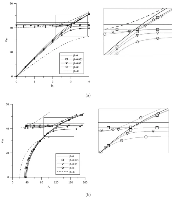
4.3.1. Effects of Inverse of Torsional Spring Coefficient, b on Natural Frequency

pinned-clamped beam or pinned–pinned beam. As can be seen from Figure 6a, the fundamental natural frequency increases with decreasing value of b. However, the second natural frequency essentially does not change for very small values of b, but for large values the frequency es. In the plots of frequency versus axial load (see Figure 6b), the fundamental frequency increas-es with decreasing valuincreas-es of b up to a certain value of the axial load, and then the trend is re-versed for higher axial loads. Nayfeh and Emam (2008) show that there is an intersection point between the first and the second natural frequencies for both clamped-clamped and pinned-pinned beams in contrast to clamped-pinned supports. This intersection point may lead to one-to-one internal resonance. Depending on the b values this intersection point may or may not exist.

0 1 2 3 4

bn

0 20 40 60

m

    

(a)

0 40 80 120 160 200



0 20 40 60

m

    

(b)

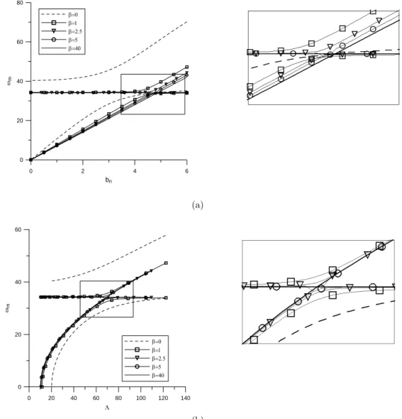
Figure 7 contains plots similar to those in Figure 6, but for pinned-elastically clamped beam. In this case the trends reverse compared to those for the clamped-elastically clamped beam. This is expected because the beam becomes stiffer (and frequencies go up) with decreasing values of b.

0 2 4 6

bn

0 20 40 60 80

m

    

(a)

0 20 40 60 80 100 120 140 

0 20 40 60

m

    

(b)

Figure 7: Effects of b values on natural frequencies (a) versus buckling amplitude (b) versus axial load (U =0.0) for pinned-elastically clamped beams.

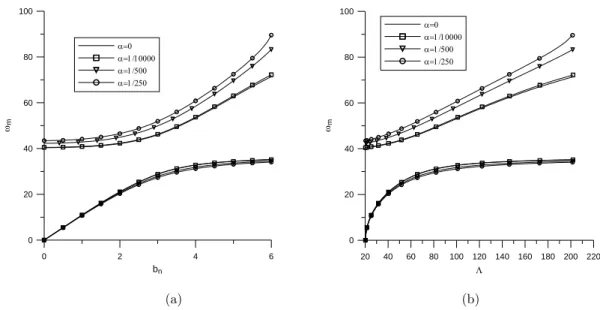
4.3.2. Effects of Inverse of Vertically Spring Coefficient of a on Natural Frequency

Figures 8a and 8b show the natural frequency versus buckling amplitude and natural frequency versus axial load, respectively, for clamped-elastically pinned beams. It can be seen from Figures 8a and 8b, that there are small differences in natural frequencies obtained with different values of

0 2 4 6

bn

0 20 40 60 80 100

m

   

20 40 60 80 100 120 140 160 180 200 220 0

20 40 60 80 100

m

   

(a) (b)

Figure 8: Effects of vertically spring coefficient on the natural frequency (a) versus buckling amplitude (b) versus axial load (U = 0) for clamped-elastically pinned beams.

4.3.3 Effects of Axial Deflection U on the Natural Frequency

The value of U =[ (0, )u t -u l t( , )] /l affects the axial load directly, If the axial deflection is

al-lowed, then lower axial load can be obtained. In Figures 9a-9c, graphs of the natural frequency versus axial load are plotted to show the effect of axial deflection for classical boundary condi-tions (i.e., CC, PP, and PC). For CC and PP boundary condicondi-tions, the natural frequencies of vibration at the second mode are almost constant. Thus, the effect of axial deflection at the sec-ond mode for these boundary csec-onditions disappears in contrast to the PC boundary csec-ondition. However, the effect of the axial deflection on the natural frequency can be seen at first mode vi-bration mode in vicinity of buckled beam.

4.3.4 Effects of Second Mode Buckling on Stability of the Beam

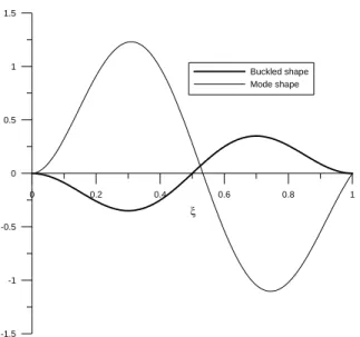
Another interesting case is the vibration about the second buckled configuration. In this case, the beam buckles at the second mode (see Figure 10). When the smallest frequency around the sec-ond buckled mode is calculated, the mode shape of the smallest frequency looks the same as the second mode shape. It is noted that the second mode is physically unstable.

5 SUMMARY AND CONCLUSIONS

are obtained by solving the linear buckling problem analytically after incorporating the nonlinear-ity into a constant. The beam is stable at its original static equilibrium position, up to the first critical load, where it loses stability by a supercritical pitchfork bifurcation. Moreover, natural frequencies are obtained in post-buckling region about buckled configuration. Some interesting results are obtained for variety of non-classical boundary conditions. When the beam is elastically clamped, at certain spring values, the mode number of the calculated natural frequencies is not identifiable. It means that a calculated natural frequency for the spring coefficients may be for either first mode or second mode. The axial deflection and slenderness ratio have meaningful ef-fects on the behavior of buckled beam. Extension of the present study using the Timoshenko beam theory is awaiting attention.

0 40 80 120 160 200

 0

20 40 60

m

U=0.0 U=0.001 U=0.005 U=0.01

0 20 40 60 80 100 120

0 10 20 30 40 50 60

m

U=0.0 U=0.001 U=0.005 U=0.01

(a) (b)

0 20 40 60 80 100

 0

10 20 30 40 50

m

U=0.0 U=0.001 U=0.005 U=0.01

(c)

Figure 9: Effects of axial deflection, U on natural frequency for h =50 when the support is (a) clamped-elastically clamped for b =0 (clamped-clamped) (b) clamped-elastically clamped for b =40 (clamped-pinned)

0 0.2 0.4 0.6 0.8 1



-1.5 -1 -0.5 0 0.5 1 1.5

Buckled shape Mode shape

Figure 10: b=0 (fixed-fixed beam), c_n =1.0 and L =10.23.

Acknowledgements

The first author acknowledges the support by National Science and Technology Foundation of

Turkey (TÜBİTAK) and the second author acknowledges the support by Higher Education

Council of Turkey (YÖK). The last author acknowledges the support of the research reported herein by the National Science Foundation research grants CMMI-1000790 and CMMI-1030836.

References

Arbind, A., Reddy, J.N., Srinivasa, A., (2014). Modified couple stress-based third-order theory for nonlinear anal-ysis of functionally graded beams. Latin American Journal of Solids and Structures 11 (3): 459-487.

Emam, S.A., Nayfeh, A.H., (2009). Post-buckling and free vibrations of composite beams. Composite Structures, 88: 636-642.

Nayfeh, A.H., Emam, S.A., (2008). Exact solution and stability of postbuckling configurations of beams. Nonline-ar Dynamics, 54: 395-408.

Nayfeh, A.H., Pai, P.F., (2004). Linear and Nonlinear Structural Mechanics. Wiley-Interscience, New York. Reddy, J.N., (2004). Mechanics of Laminated Plates and Shells, Theory and Analysis, 2nd ed., CRC Press, Boca Raton, FL.

Reddy, J.N., (2007). Theory and Analysis of Elastic Plates and Shells, 2nd ed., CRC Press, Boca Raton, FL. Reddy, J.N., Mahaffey, P., (2013). Generalized beam theories accounting for von Kármán nonlinear strains with application to buckling. Journal of Coupled Systems and Multiscale Dynamics, 1(1): 120-134.

Shen, H.S., (2011). A novel technique for nonlinear analysis of beams on two-parameter elastic foundation. Inter-national Journal of Structural Stability and Dynamics, 11(6): 999-1014.

Sinir, B.G., (2010). Bifurcation and chaos of slightly curved pipes. Mathematical and Computational Applications, 15(3): 490-502.