Abs tract
The effect of viscoelasticity of epoxy adhesive on creep behavior in the adhesive layer of a double-lap joint is studied in this paper. The joint is comprised of three elastic single isotropic adherend layers joined by an epoxy adhesive that is under shear loading. Prony series is used to modeling the relaxation modulus of epoxy adhesive. The differential equation is derived in Laplace domain, and numerical inversion from the Laplace domain to the time domain is achieved by the Fixed Talbot method. Results show that for an impulse load of 100N, maximum shear stress in the adhesive layer is reduced to 38% of its initial value after almost 12 days and 79% of its initial value over a very long time. The rate of increase in tensile load P has a direct effect on peak shear stress developed in the adhesive layer and holding P0 as a constant, increasing will lower the induced peak shear stress in the joint. Also, an in-crease in the thickness of the adhesive layer reduced the induced peak shear stress and strain in the joint.
K ey words
Adhesive Joint, Double-Lap joint, Epoxy, Inverse Laplace Trans-form, Viscoelasticity, Fixed Talbot Method.
The Effect of Viscoelasticity on Creep Behavior of
Double-Lap Adhesively Bonded Joints
1 INTRODUCTION
The most structurally efficient method of connecting the structures is to use shear joints, which are either adhesively bonded or mechanically fastened. The use of adhesives has many advantages over other methods of fastening. Presenting a smooth exterior, spreading of the load and ease of joining thin or dissimilar materials are all reasons why the use of adhesives for bonding structures is steadi-ly growing and finding new applications (Adams, Comyn and Wake, 1997). Adhesive bonded joints are already playing a significant role in the development and production of various industries. When used to bond polymers or polymer-matrix composites, the adhesives can be selected from the same family of materials to assure good compatibility (de Geramo, Black and Kohser, 1997). However, adhesives are flaw dominated and due to their viscoelastic character, time-dependent failures
prob-A r as h R e za*, Moh am ma d Sh i sh es az an d K h os ro N ad e ra n-Ta han
Department of Mechanical Engineering, Shahid Chamran University of Ahvaz, Iran
Received in 03 Nov 2012 In revised form 11 Apr 2013
Latin American Journal of Solids and Structures 11(2014) 035 - 050
ably occur. Thus, in the design of adhesively bonded joints, to ensure their safety, it is necessary to examine stress distribution developed in the joint. Many of researchers have performed different theoretical analyses for single-lap and double-lap adhesive joints. They provided considerable eluci-dations of the qualitative behavior of joints under load. The theoretical analyses are based on cer-tain simplifications in order to achieve tractable results and the consequent quantitative agreement with experiments.
An extensive literature review on existing analytical models for both single and double-lap joints has been made by Baldan (2004) and da Silva et al. (2009) to assist the designer to choose the right model for a particular application. A simplified one-dimensional approach has been developed by Her (1999) to model the adhesive bonding for single-lap joint and double-lap joint. He obtained good agreement between a simply analytical solution and the two-dimensional finite element results. In his study, the effects of varying parameters such as thickness of adhesive and adherend, modulus of adhesive and adherend have been investigated. Khalili et al. (2008) studied the response of single-lap joints with composite adherends subjected to in-plane as well as out-of-plane normal loads by means of 3D finite element technique using ANSYS software. They showed that changing the orien-tation of fibers in the adhesive region with respect to the global axes influenced the bond strength. Tsai and Morton (2010) investigated the stress distributions and mechanics of the laminated com-posite double-lap joints with unidirectional and quasi-isotropic adherends by experimental, numeri-cal and theoretinumeri-cal analyses. Experimental and finite element results suggest that the laminated composite double-lap joints have significant adherend shear deformations, which have been neglect-ed in the theoretical modeling. Many studies on failure analysis of a family of adhesive single-lap joints have been performed analytically and experimentally by da Costa Mattos et al. (2011 and 2012). da Costa Mattos et al. (2011) proposed a phenomenological framework to perform the failure analysis of adhesive single-lap joints. They considered quasi-brittle behaviour for epoxy/ceramic composite adhesive and highly resistant behaviour for ASTM A36 steel adherends and predicted the rupture force of adhesive joints. da Costa Mattos et al. (2012) proposed a shape factor that allows correlating the static strength of two single-lap joints with different geometries. da Costa Mattos et al. (2012) in the following of their researches, studied failure analysis, rupture forces and lifetimes of composite adhesive single-lap joints.
Latin American Journal of Solids and Structures 11(2014) 035 - 050 the adherend as linearly elastic. The geometric nonlinearity in the single-lap joint was due to finite rotation of the joint. The stress-strain of the adhesive material is modeled by the Ramberg-Osgood equation. Viscoplastic analysis gives the reduced stresses at the end of overlap than the elastic solu-tion.
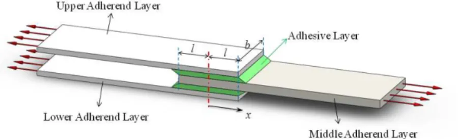
In this paper, the effect of viscoelasticity of an epoxy adhesive on shear stress distribution and creep behavior in the adhesive layer of a double-lap joint is studied. The factors accounted for in this analysis over that published previously, include adhesive viscoelasticity and a semi-analytical solution. The proposed model is consisted of three dissimilar adherend layers joined by an adhesive layer, as shown in Figure 1.
Figure 1 A Double-lap joint under tension.
Each adherend layer is modeled as linear elastic while for adhesive layer, a linear viscoelastic be-havior is assumed. Prony series is usedto modeling the relaxation shear modulus of an epoxy adhe-sive and governing equilibrium equations are derived in the Laplace domain. Because of intricacy of governing equation in the Laplace domain, Fixed Talbot method was used to inverse this equation into time domain.
2 GOVERNING EQUATIONS IN THE ADHESIVE LAYERS
The following assumptions are used for modeling the problem: Stress is applied only in the x direction.
Behavior of adherend layer is assumed to be linear elastic. Linear viscoelastic material is assumed as an adhesive.
The Prony series is used for modeling the shear relaxation behavior of the adhesive. The adhesive does not carry any significant axial force.
Due to the state of plane stress condition, Out-of-plane normal stresses are ignored in both the adhesive and adherend layers (Dillard and Pocius, 2002).
The effect of bending moment developed by the applied forces in the joint is ignored. It is also assumed that the shear stress in the adhesive layer is constant along the joint width. Moreover, it is assumed that ∂v ∂x is negligible compared to ∂u ∂y (v is vertical deformation in adhesive along y direction). Using this assumption along with a linear distribution for axial defor-mation “u” along the adhesive thickness, leads into the fact that shear stress at any section along the thickness of the adhesive layer remains constant (τ
Latin American Journal of Solids and Structures 11(2014) 035 - 050
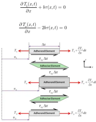
assumption, as shown in Figure 2, a force balance on each adherend layer of the joint, with a length Δx, leads into;
∂T 1(x,t)
∂x +
bτ(x,t)=0 (1a)
∂T o(x,t) ∂x
−2bτ(x,t)=0 (1b)
Figure 2 Force balance on an element of the joint.
In Eq. (1), b refers to the width of the joint (see Figure 1). According to the symmetric model,
T
1(x,s)= T
2(x,s), thus, the relations that imply to the bottom adherend will be neglected. Moreo-ver, assuming linear elasticity, the strain in each adherend layer may be written as;
ε
1(x,t)= ∂u
1(x,t) ∂x
where ε
1(x,t)= T
1(x,t) E
1d1b
(2a)
ε
o(x,t)= ∂u
o(x,t)
∂x
where ε
o(x,t)= T
o(x,t) E
odob
(2b)
Subscripts 0, 1 and 2 refer to the properties associated with the middle, upper and lower ad-herend layers respectively. Geometry of this model is shown in Figure 3. According to Eq. (2), one may write;
∂u 1(x,t)
∂x =
T 1(x,t) E
1d1b
, ∂uo(x,t)
∂x =
T o(x,t) E
odob
Latin American Journal of Solids and Structures 11(2014) 035 - 050 Figure 3 Geometry of the Adhesively Double-Lap joint.
As a first approximation, the adhesive shear strain is taken as;
γ(x,t)= u
o(x,t)−u1(x,t) h
1
(4)
Where, h
1 is the adhesive thickness between top and middle adherends. For epoxy adhesive with viscoelastic properties, the relationship between shear stress and strain is as follows (Drezdov, 1998):
τ(x,t)=
0 t
∫
G(x,ς)∂γ(x,ς) ∂ςdς (5)
In Eq. (5), τ(x,t) is the shear stress, G and γ are the adhesive relaxation shear modulus and
shear strains respectively, and
ς
is the variable of integration. Using the Laplace transform, Eq. (5) may be written as; τ(x,s)=
G∗
(s)γ(x,s)=s
G(s)γ(x,s) (6)
This result of the same form as Hooke’s law for a linear elastic material and is sometimes called Alfrey’s Correspondence Principle (Brinson, 2008). The quantityG∗
(s), in transform space is
analo-gous to the usual Young’s shear modulus for a linear elastic material. Here, the linear differential relation between stress and strain for a viscoelastic polymer has been transformed into a linear elas-tic relation between stress and strain in the transform space. Moreover, in Laplace domain, Eqs. (1) – (4) may be written as;
∂
T
1(x,s) ∂x
+bτ(x,s)=0 (7a)
∂
T
o(x,s)
∂x
−bτ(x,s)=0 (7b)
∂u 1(x,s)
∂x =
T
1(x,s) E
1d1b , ∂
u
o(x,s)
∂x =
T
o(x,s) E
odob
Latin American Journal of Solids and Structures 11(2014) 035 - 050
γ(x,s)=
u
o(x,s)−
u 1(x,s) h
1
(9)
Upon differentiating Eqs. (6) and (7a), one may write;
∂τ(x,s) ∂x
=s
G(s)
h
1
∂u o(x,s) ∂x −
∂u
1(x,s)
∂x ⎛ ⎝ ⎜⎜ ⎜⎜ ⎞ ⎠ ⎟⎟ ⎟⎟ (10) ∂2 T 1(x,s) ∂x2
=−b∂
τ(x,s)
∂x (11)
Substituting Eq. (10) back into (11) we have;
∂2
T
1(x,s)
∂x2
=−s G(s)b
h 1
∂u
o(x,s) ∂x −
∂u 1(x,s)
∂x ⎛ ⎝ ⎜⎜ ⎜⎜ ⎞ ⎠ ⎟⎟ ⎟⎟=− s G(s)b
h 1
T
o(x,s)
E
odob −
T
1(x,s) E
1d1b
⎛ ⎝ ⎜⎜ ⎜⎜ ⎞ ⎠ ⎟⎟ ⎟⎟ (12) Since;
To(x,s)=
P(s)−2
T
1(x,s) (13)
Then, substituting for T
o(x,s) from Eq. (13) back into Eq. (12) gives;
∂2
T 1(x,s) ∂x2 −
s
G(s)
h 1
2 E
odo
+ 1
E 1d1 ⎛ ⎝ ⎜⎜ ⎜⎜ ⎞ ⎠ ⎟⎟ ⎟⎟ T
1(x,s)=− s
G(s)
P(s)
E odoh1
(14)
The following boundary conditions are used to solve Eq. (14).
T
1(l,s)=0 &
T
1(−l,s)=
P(s)
2 (15)
Upon proper application of boundary conditions, one may write;
T
1(x,s)= P(s)
2 −
1 2
sinh(λ(s)x) 2sinh(λ(s)l)
+1
2 E
odo−2E1d1
E
odo +2E1d1
⎛ ⎝ ⎜⎜ ⎜⎜ ⎞ ⎠ ⎟⎟ ⎟⎟ ⎡ ⎣ ⎢ ⎢
cosh(λ(s)x) cosh(λ(s)l)
+ 2
E 1d1 E
odo+2E1d1
⎤ ⎦ ⎥ ⎥ (16a) T
o(x,s)=
P(s) 1+1 2
sinh(λ(s)x)
sinh(λ(s)l) −
1 2
E
odo−2E1d1
E
odo +2E1d1 ⎛ ⎝ ⎜⎜ ⎜⎜ ⎞ ⎠ ⎟⎟ ⎟⎟ ⎡ ⎣ ⎢ ⎢
cosh(λ(s)x)
cosh(λ(s)l)−
2E
1d1
E
odo +2E1d1 ⎤
⎦ ⎥
Latin American Journal of Solids and Structures 11(2014) 035 - 050 Where
λ(s)=c s
G(s) & c = 1
h 1
2 E
odo
+ 1
E 1d1 ⎛
⎝ ⎜⎜ ⎜⎜
⎞
⎠ ⎟⎟
⎟⎟ (17)
With the help of Eq. (1), shear stress in the adhesive layer may be expressed as:
τ(x,s)= P(s)λ(s)
4
cosh(λ(s)x) sinh(λ(s)l) −
E
odo−2E1d1 E
odo +2E1d1 ⎛
⎝ ⎜⎜ ⎜⎜
⎞
⎠ ⎟⎟ ⎟⎟sinh(
λ(s)x)
cosh(λ(s)l) ⎡
⎣ ⎢ ⎢
⎤
⎦ ⎥
⎥, −l <x <l (18)
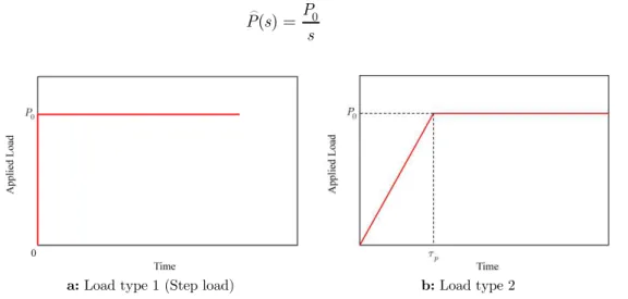
Where at x = +l,−l, τ(x,s)=0. In this study two different type of loading conditions are con-sidered. In the first case, the applied load (see Figure 4a) is expressed as a step function P(t)=P
0, where, in Laplace domain it may be represented by Eq. (19) as;
P(s)= P0
s (19)
a: Load type 1 (Step load) b: Load type 2
Figure 4 Types of loadings applied to the joint. In the second case, the ramp portion of the load occurs at 0≤t ≤τ
p, and afterward it remains constant (see Figure 4b). Here, the applied load in the Laplace domain may be expressed as in Eq. (20).
P(s)= P0 τ
p
1−e−τps
s2 ⎛
⎝ ⎜⎜ ⎜⎜⎜
⎞
⎠ ⎟⎟ ⎟⎟
⎟⎟ (20)
Latin American Journal of Solids and Structures 11(2014) 035 - 050
τ(x,s)= αP(s) s
G(s) cosh c s
G(s)x
(
)
sinh c s
G(s)l
(
)
−βsinh c s
G(s)x
(
)
cosh c s
G(s)l
(
)
⎡ ⎣ ⎢ ⎢ ⎢ ⎢ ⎤ ⎦ ⎥ ⎥ ⎥ ⎥, −l <x <l (21)
In Eq. (21),
a
and b are constants defined as in Eq. (22).α= c
4b, β = E
odo−2E1d1 E
odo +2E1d1
⎛ ⎝ ⎜⎜ ⎜⎜ ⎞ ⎠ ⎟⎟ ⎟⎟ (22)
Now, Eq. (6) is used to calculate the creep response of the adhesive layer. Hence, the shear strain may be written as;
γ(x,s)=
τ(x,s)
s
G(s) (23)
Replacing Eq. (21), in (23), shear strain in the adhesive layer in Laplace domain is equal to;
γ(x,s)= α P(s) s
G(s)
cosh(c s G(s)x)
sinh(c s G(s)l) −
βsinh(c s
G(s)x)
cosh(c s
G(s)l)
⎡ ⎣ ⎢ ⎢ ⎢ ⎤ ⎦ ⎥ ⎥ ⎥ (24)
Taking the inverse Laplace transform of Eq. (24), an expression for creep as a function of time in adhesive layer is obtained. The Prony series with 10 terms is used to model the relaxation modulus of epoxy resin (Wang, 2009). Prony series, as expressed in Eq. (25), is used to represent the viscoe-lastic behavior of the adhesive layer in time domain.
G(t)=G∞ + G
ie −t τ i i 10
∑
(25)For replacing the relaxation shear modulus in Eq. (24), the Prony series must be expressed in the Laplace domain that can be written as;
G(s)=G∞
s +
Giτi
τ
is +1
i
10
∑
(26)Latin American Journal of Solids and Structures 11(2014) 035 - 050 3 INVERSE LAPLACE TRANSFORM BY FIXED TALBOT METHOD
Eq. (24) may be written in time domain as in Eq. (27) that is known as Bromwich integral.
γ(x,t)= 1
2πi
C
∫
estγ(x,s)ds (27)Due to the complexity of the governing relations of the stress and strain in the Laplace domain, using analytical methods of the inverse Laplace transform is not possible. This is one of the usual problems in solving the viscoelastic problems of complex models. By taking viscoelasticity, the stress and strain in the adhesive layer is a function of position and time. According to the presented topics in this study, one can easily obtain stress and strain in the adhesive layer in terms of position and the Laplace variable of s. Therefore, for calculating stress and strain in the adhesive layer in a particular time, the numerical algorithms of inverse Laplace transform are used. General form of the numerical inverse Laplace transform [21] is defined in relation (28).
f(t)≈ fn(t)= 1
t Re
ω k
f(αk
t ) ⎡
⎣ ⎢ ⎢
⎤
⎦ ⎥ ⎥ k=0
n
∑
, t >0 (28)Where,
f(s) is Laplace transformation of f(t) for the real positive values of time t >0 and
f(t) can be obtained by a linear combination of limited terms of transformed function f(s) multi-plying in the inverse of time and also the replacement of αk
t instead of Laplace variable. Thus, to calculate f(t), it is sufficient to obtain the amount of desired function in the Laplace domain at αk
t
fork =0…n. In most of cases, the coefficients of α
k and ωk are a complex number that depends on the amount of n. The accuracy of approximation is depending on the number of applied terms in relation (28). Several algorithms (Montella, 2009) such as Gaver-Stehfest method, Euler method, Fixed Talbot method and Durbin method can be expressed in the mentioned general form in the relation (28). In this study Fixed Talbot method has been used to calculate the inverse of shear stress transformed function in the Laplace domain.
The Fixed Talbot (FT) algorithm has been caused from the Bromwich inverse integral; hence it needs complex computations. Inverse transform in this method is approximated with the help of the following relations.
f(t)≈ fM(t)= 2
5t Re γk
f(δk
t )
⎡
⎣ ⎢ ⎢
⎤
⎦ ⎥ ⎥ k=0
M−1
∑
, t >0 (29)Latin American Journal of Solids and Structures 11(2014) 035 - 050
θk =kπ M,
δ0 =2M 5,
δk =δ0θk⎡⎣cot(θk)+i⎤⎦
γ0 =0.5 exp(δ0),
γk ={1+iθ
k 1+(cot(θk)) 2 ⎡
⎣⎢ ⎤⎦⎥−icot(θk)}exp(δk), 0<k <M
(30)
The Fixed Talbot method is a case of general form of the relation (28), where n =M−1,
α
k =δk and ωk = 2
5γk.
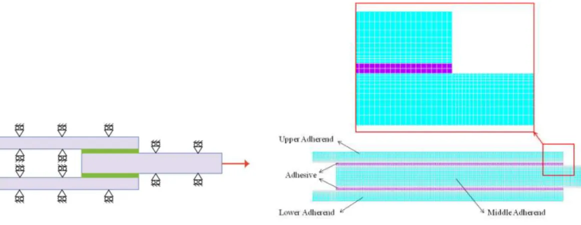
4 FINITE ELEMENT ANALYSIS
Finite element model of the joint was prepared and solved for stress distribution in the adhesive layer using ANSYS v11. Each adherend and adhesive layer was meshed using PLANE183 element. This is an 8-node element and has quadratic displacement behavior and may be used as a plane element in plane stress, plane strain and generalized plane strain conditions. The Prony series in different form as expressed in Eq. (31), is used to apply for implement the viscoelastic properties of the adhesive layer in ANSYS.
G(t)=G0 λ ∞+
j=1 N
∑
λje
−t/τ
j
⎡
⎣ ⎢ ⎢ ⎢
⎤
⎦ ⎥ ⎥
⎥ (31)
The initial shear elastic modulus G0 and λj are defined as
G0 =G∞+
j=1
N
∑
Gj, λ j =Gj
G∞ (32)
λ
Latin American Journal of Solids and Structures 11(2014) 035 - 050
a: Finite element model of the lap joint b: Portion of the meshed model
Figure 6 Finite element model of the joint and its meshed state.
5 RESULTS AND DISCUSSION
The main objective of this work is to determine the shear stress distribution and creep response of epoxy adhesives under shear. As indicated by equilibrium equations, for a double-lap joint under shear, stress distribution in the adhesive is a function of physical and mechanical properties of all constituents. The results in this section are based on an overlap length of 20 mm, with 1 mm thick Aluminum adherend layers glued to 0.01-0.1 mm thick epoxy adhesive. Material properties for each layer are selected according to Table 1 and 2. The applied load is taken to be 100 N.
Table 1 Mechanical and physical properties of adherend and adhesive layers
Material E (GPa) ν Thickness, h (mm) Width, b (mm) Overlap, 2l (mm)
Adherends: Aluminum 69 0.33 1 40 20
Adhesive: Epoxy 3.2 0.4 0.01-0.1 40 20
Latin American Journal of Solids and Structures 11(2014) 035 - 050
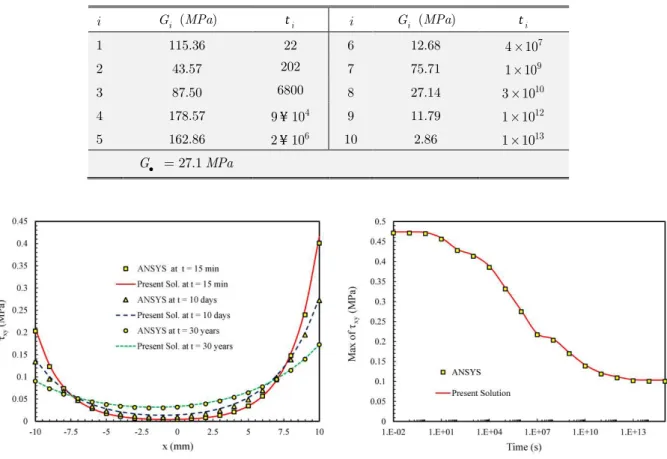
Table 2 The parameters of the Prony series describing the shear relaxation modulus function of epoxy adhesive (Wang, 2009)
i Gi (MPa) ti i Gi (MPa) ti
1 115.36 22 6 12.68 4×10⁷
2 43.57 202 7 75.71 1×10⁹
3 87.50 6800 8 27.14 3×10¹⁰
4 178.57 9 104
¥ 9 11.79 1×10¹²
5 162.86 6
2¥10 10 2.86 1×10¹³
27.1
G MPa • =
Figure 7 Comparison of finite element and present analysis on shear stress in the adhesive layer
Figure 8 Comparison of maximum shear stress vs. time
Figure 9 shows the effect of viscoelasticity of the adhesive layer on shear stress produced along the joint due a step load (type 1) applied to the joint. For further comparison, the results based on elastic behavior of the joint (Her, 1999) are superimposed.
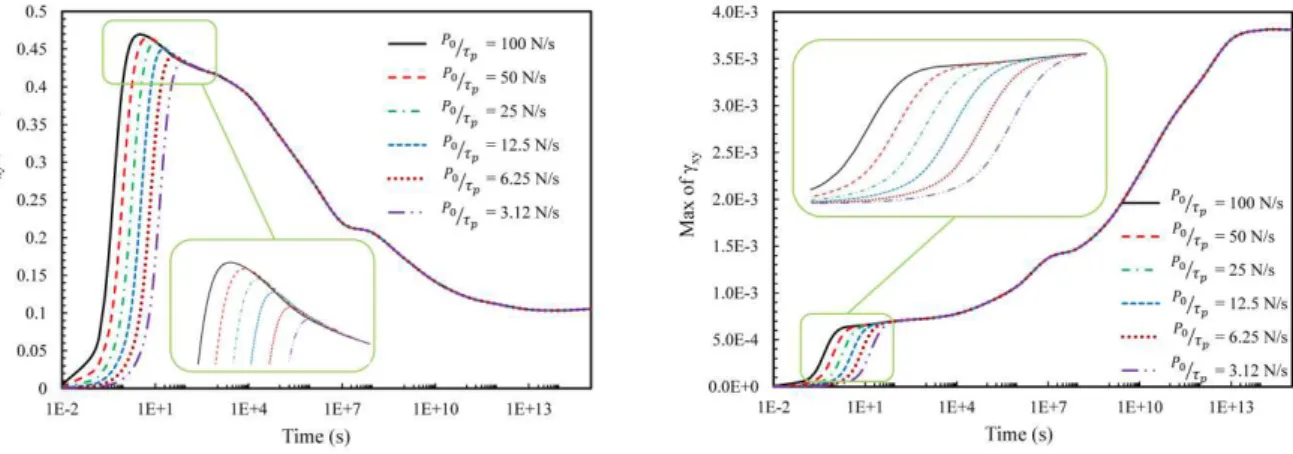
Latin American Journal of Solids and Structures 11(2014) 035 - 050 According to this figure, linear elasticity solution matches those of viscoelastic solution at time equal to zero. For example, as time elapses to almost 12 days, the magnitude of peak shear stress is reduced substantially to about 38% of its initial value, and is reduced to 79% over a very long time. According to Figure 10, the rate of increase in tensile load P has a direct effect on peak shear stress developed in the adhesive layer. For example, increasing the loading rate from 3.12 to 100 N/s will increase the maximum shear stress in the joint by almost 12%. This means that holding P0 as a constant, increasing τ
p will lower the induced peak shear stress in the joint. According to Figure
11, lowering the loading rate will manifest itself in a more gradual rise in the shear strain developed in adhesive layer. But, the loading rate hasn't any effect on the peak shear strain.
Figure 10 The effect of loading rate on the maximum shear stress developed in the adhesive layer
Figure 11 The effect of loading rate on the maximum shear strain developed in the adhesive layer
The adhesive thickness appears to have considerable effect on the shear strain (stress) developed in the adhesive layer. According to Figure 12, increasing the thickness of the adhesive layer from 0.01 to 0.1 mm, lowers the peak shear strain in the joint to almost 31% of its initial value.
a: Left side of the adhesive layer b: Right side of the adhesive layer
Latin American Journal of Solids and Structures 11(2014) 035 - 050
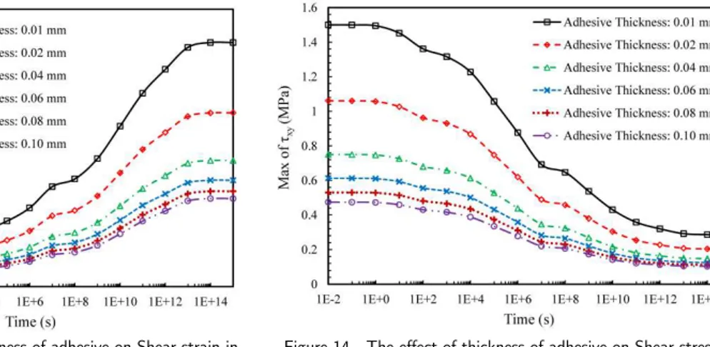
Due to viscoelastic behavior of the adhesive layer, after a certain time period, any elapse in time will cause noticeable rise in the adhesive layer shear strain. This variation is shown in Figure 13 for different adhesive thicknesses.
Figure 13 The effect of thickness of adhesive on Shear strain in the adhesive with respect to time (load type 1)
Figure 14 The effect of thickness of adhesive on Shear stress in the adhesive with respect to time (load type 1)
According to this figure, it appears that the shear strain reaches its steady value over a very long time regardless of the adhesive thickness. For load type 1, any increase in shear strain over time manifests itself to smaller values of shear stress in the joint (see Figure 14). According to this figure, as the adhesive layer is thickened from 0.01 to 0.1 mm, the peak stress developed in the ad-hesive layer is decreased by 67% at time zero and this ratio of decreasing will be constant after ex-tra amount of time. Thus, the effect of glue thickness on the induced shear stress in the adhesive layer is more pronounced at t = 0.
Figure 15 The effect of thickness of adhesive on Shear stress in the adhesive layer with respect to over time
(load type 2 with τ
p = 16s)
Figure 16 The effect of thickness of adhesive on Shear strain in the adhesive layer with respect to over time
(load type 2 with τ p =
16s)
adhe-Latin American Journal of Solids and Structures 11(2014) 035 - 050 sive thickness. Based on the given data in table 1 & 2, the peak shear stress occurs at about t = 100 seconds. The peak values of shear stress for load type 2 seem to be in the same range as those for type 1. Also, according to Figure 16, for load type 2, the peak shear strain in the adhesive layer has a same trend for all values of adhesive thickness.
5 CONCLUSION
This paper presents an analytical study on the shear strain and stress distribution in a viscoelastic adhesive layer of a double-lap joint under tension. The shear-lag model has been used to obtain governing equilibrium equations. The differential equation is derived in Laplace domain, and nu-merical inversion from the Laplace domain to the time domain is achieved by the Fixed Talbot method. At time zero, the results based on elastic analysis of all constituents match those obtained in this work. Also, according to the results, for a step load of P0 = 100 N, the maximum shear stress in the adhesive layer is reduced to 38% of its initial value after almost 12 days and is reduced to 79% of its initial value over a very long time.Moreover, if the applied load is gradually increased to a final value of P0, its rate of increase has a direct effect on the peak shear stress developed in the adhesive layer. For both types of loads, increase in thickness of the adhesive layer from 0.01 to 0.1 mm caused a decreased in the adhesive peak shear stress and strain. According to the results, for both types of loads, the peak values of shear stress and strain seem to be in the same range.
References
Adams, R.D., Comyn, J., Wake, W.C., (1997). Structural Adhesive Joints in Engineering, Chapman Hall (Lon-don).
De Garmo, E.P., Black, J.T., Kohser, R.A., (1997). Materials and Processes in Manufacturing, Prentice-Hall (New York).
Baldan, A., (2004). Review Adhesively-Bonded Joints in Metallic Alloys, Polymers and Composite Materials: Me-chanical and Environmental Durability Performance, Journal of Materials Science 39: 4729–4797.
da Silva, L.F.M., Dasneves, P.J.C., Adams, R.D., Spelt, J.K., (2009). Analytical Models of Adhesively Bonded Joints - Part I: Literature Survey, International Journal of Adhesion & Adhesives 29: 319-330.
Her, S. (1999). Stress Analysis of Adhesively-Bonded Lap Joints, Journal of Composite & Structures 47: 673-678. Khalili, S.M.R., Khalili, S., Pirouzhashemi, M.R., Shokuhfar, A., Mittal, R.K., (2008). Numerical study of lap joints with composite adhesives and composite adherends subjected to in-plane and transverse loads, International Journal of Adhesion & Adhesives 28: 411–418.
Tsai, M.Y., Morton, J., (2010). An investigation into the stresses in double-lap adhesive joints with laminated composite adherends, International Journal of Solids and Structures 47: 3317–3325.
da Costa Mattos, H.S., Sampaio, E.M., Monteiro, A.H., (2011). Static failure analysis of adhesive single lap joints, International Journal of Adhesion & Adhesives 31: 446–454.
da Costa Mattos, H.S., Monteiro, A.H., Palazzetti, R., (2012). Failure analysis of adhesively bonded joints in com-posite materials, J. Material & Design 33: 242–247.
da Costa Mattos, H.S., Sampaio, E.M., Monteiro, A.H., (2012). A simple methodology for the design of metallic lap joints bonded with epoxy/ceramic composites, J. Composites, Part B 43: 1964–1969.
Dillard, D.A., Pocius, A.V., (2002). Adhesion Science and Engineering – I: The Mechanics of Adhesion, Elsevier Science B.V (London).
Latin American Journal of Solids and Structures 11(2014) 035 - 050
Ferry, J.D., (1980). Viscoelastic Properties of Polymers, John Wiley & Sons Inc. (Toronto).
Yadagiri, S., Reddy, C.P., Reddy, T.S., (1987). Viscoelastic Analysis of Adhesively Bonded Joints, J. Composite & Structures 27(4): 445-454.
Groth, H.L., (1990). Viscoelastic and Viscoplastic Stress Analysis of Adhesive Joints, International Journal of Ad-hesion & Adhesives 10(3): 207-213.
Pandey, P.C., Narasimhan, S., (2001). Three-Dimensional Nonlinear Analysis of Adhesively Bonded Lap Joints Considering Viscoplasticity in Adhesives, J. Composite & Structures, 79: 769-783.
Drezdov, A.D., (1998). Mechanics of Viscoelastic Solids, John Wiley & Sons (London).
Brinson, H.F. and Brinson, L.C., (2008). An Introduction to Polymer Engineering Science & Viscoelasticity, Springer (New York).
Wang, Y. (2009). Integrated measurement technique to measure curing process-dependent mechanical and thermal properties of polymeric materials using fiber bragg grating sensors, Ph.D. Thesis, College Park, University of Mary-land, USA.
Montella, C. and Diard, J.P., (2008). New approach of electrochemical systems dynamics in the time-domain under small-signal conditions. I. A family of algorithms based on numerical inversion of Laplace transforms, J. Electroan-alytical Chemistry 623: 29–40.