ISSN 0101-8205 www.scielo.br/cam
Rheodynamic lubrication of a squeeze film bearing
under sinusoidal squeeze motion
A. KANDASAMY∗ and K.P. VISHWANATH∗∗
Department of Mathematical and Computational Sciences
National Institute of Technology Karnataka, Surathkal, Mangalore – 575.025, India
E-mails: [email protected] / [email protected]
Abstract. Lubricants with variable viscosity are assuming importance for their applications in
polymer industry, thermal reactors and in biomechanics. With the bearing operations in machines
being subjected to high speeds, loads, increasing mechanical shearing forces and continually
increasing pressures, there has been an increasing interest to use non-Newtonian fluids
character-ized by an yield value. The most elementary constitutive equation in common use that describes
a material which yields is that of Bingham fluid. In the present work, the problem of a circular
squeeze film bearing lubricated with Bingham fluid under the sinusoidal squeeze motion has been
analyzed. The shape and extent of the core for the case of sinusoidal squeeze motion has been
determined numerically for various values of the Bingham number. Numerical solutions have
been obtained for the bearing performances such as pressure distribution and load capacity for
different values of Bingham number, Reynolds number and for various amplitudes of squeeze
motion. The effects of fluid inertia, non-Newtonian characteristics, and the amplitudes of squeeze
motion on the bearing performances have been discussed.
Mathematical subject classification:76A05, 76D08.
Key words: non-Newtonian fluid, Bingham fluid, yield stress, rheodynamic lubrication,
squeeze film bearing, sinusoidal motion.
#726/07. Received: 01/II/07. Accepted: 24/V/07.
∗Professor and Head
1 Introduction
Recently, it has been emphasized that in order to analyze the performance of bearings adequately, it is necessary to take into account the combined effects of fluid inertia and non-Newtonian characteristics of lubricants. In most squeeze film bearings, the effects of fluid inertia forces become significant with increase in squeeze velocity as well as film thickness.
The effects of fluid inertia forces and non-Newtonian characteristics of lubri-cants in the squeeze film bearings have been examined by several investigators, (Tichy and Winer [8], Covey and Stanmore [2], Gartling and Phan-Thien [4], Donovan and Tanner [7], Huang et al. [6], Usha and Vimala [9]) but there are few papers attempting to describe the combined effects of fluid inertia forces and non-Newtonian characteristics of lubricants (Elkough [3], Batra and Kan-dasamy [1]) . Even these works are without considering the sinusoidal motion of the squeeze film bearing. With sinusoidal squeeze motion, Usha and Vimala [10] have applied the energy integral approach to find the behavior of curved squeeze film bearing using a Newtonian lubricant. Hashimoto and Wada [5] have examined the effects of fluid inertia forces in a squeeze film bearing with sinusoidal motion lubricated using a power law fluid.
2 Mathematical formulation of the problem
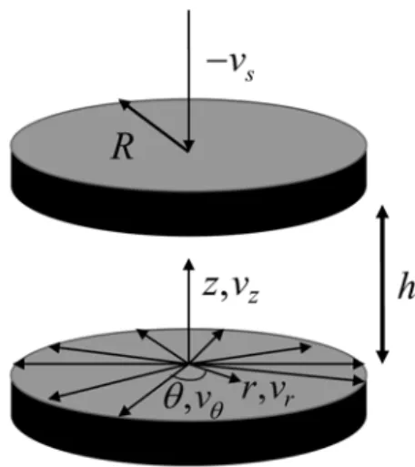
The geometry of the problem is as shown in Fig. 1. We consider an isothermal, incompressible, steady flow of a time independent Bingham fluid squeezed be-tween two circular plates separated by a distanceh. Let 2Rbe the diameter of the bearings approaching each other with a squeeze velocityvs under a normal load
W. We consider cylindrical polar co-ordinates(r, θ,z)with axial symmetry and the origin fixed at the center of the lower plate. Herer represents the distance measured along the radial direction and z along the axis normal to the plates. Letvrandvzrepresent velocity components in the radial (r) and axial directions
(z) respectively. Let pdenote the pressure andρ the density of the fluid. It is assumed that there is no sliding motion of the two plates.
Figure 1 – Geometry of the squeeze film bearing.
The constitutive equation of a Bingham fluid is given by,
τi j =2
η1+ η2 I12
ei j,
1
2τi jτi j ≥η
2 2
(1)
whereτi j are the deviatoric stress components, η1 andη2are constants named
the plastic viscosity and yield value respectively,ei j represents the rate of defor-mation components andI =2ei jei j is strain invariant.
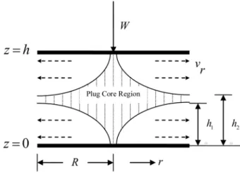
In those regions of the film, where the shear stress is less than the yield value, there will be core formation, which will move with constant velocityvc. Let the
Figure 2 – Shape of the core.
Applying the basic assumptions of lubrication theory for thin films, the gov-erning equations for the above squeeze film system, including inertia forces, is given by:
ρ
vr ∂vr
∂r +vz ∂vr
∂z
= −∂p ∂r +
∂τr z
∂z (2)
∂p
∂z = 0 (3)
1
r ∂(rvr)
∂r + ∂vz
∂z = 0 (4)
τr z = η2+η1
∂vr ∂z
(5)
The above equations (2), (3) and (5) together with the continuity equation (4), are to be solved under the following boundary conditions:
vr = 0 at z = 0,h
vz = −vs at z = h
vz = 0 at z = 0
p = pa at r = R
(6)
vr and ∂v∂zr are continuous at z = h1(r)and z = h2(r). Here pa is the
3 Solution to the problem
The integral form of the continuity equation, also called the equation of squeeze motion is given by,
2πr
h
0
vrd z=πr2vs (7)
Averaging the inertia terms in the momentum equation (2) by assuming it to be a constant over the film thickness (Hashimoto and Wada [5]), and performing integration by parts in the resulting equation using the continuity equation (4) and boundary conditions, we get,
ρ h r 2 ∂vs ∂t + ∂ ∂r h 0
vr2d z+1 r
h
0 vr2d z
+d p dr =
∂τr z
∂z (8)
Here, we introduce the following modified pressure gradient:
f ≡ ρ h r 2 ∂vs ∂t + ∂ ∂r h 0
vr2d z+1 r
h
0 vr2d z
+d p
dr (9)
Hence, from equations (8) and (9), we have,
∂τr z
∂z = f (10)
As the modified pressure gradient is independent of the coordinate z, equa-tion (10) can be integrated as follows:
τr z = f z+c1 (11)
Substitutingτr zfrom equation (11) into equation (5) and integrating the result-ing equations usresult-ing the boundary conditions (6), we get the velocity distribution in the two flow regions separating the core region as,
vr = f η1
z2
2 −h1z
in 0≤z≤h1(r) (12)
vr = f η1
z2
2 −
h2
2 −h2z+h2h
in h2(r)≤z ≤h (13)
and the core velocity as,
vr =vc = − f η1
h21
2
= − f η1
(h−h2)2
2
From equation (14), we have,
h1(r)=h−h2(r) (15)
Considering the equilibrium of an element of the core in the fluid, we get,
f = −2η2
H (16)
where
H = H(r)=h2(r)−h1(r) (17)
represents the thickness of the core.
Using the velocity equations (12), (13), (14) and the equation of squeeze mo-tion (7), we get,
f = − 12rη1vs
H3−3h2H +2h3 (18)
Eliminating f from equations (16) and (18), we get an algebraic equation for determining the thickness of the core as,
H3−3
h2−2rη1vs η2
H+2h3=0 (19)
Further, Substituting for f from equation (18) in the velocity equations (12), (13) and (14), we get,
vr =
6rvs(h−H −z)z
(h−H)2(2h+H) in 0≤z ≤h1(r) (20) vr =
3rvs
2(2h+H) in h1(r)≤z ≤h2(r) (21)
vr =
6rvs(h−z)(−H+z)
(h−H)2(2h+H) in h2(r)≤z ≤h (22)
Substitutingvr from equations (12), (13) and (14) into equation (9), we obtain the following equation for pressure gradient:
d p
dr = f − ρr
2h
∂vs ∂t
−63H
2+198H h+144h2−21r H H′−6r h H′ 20(H+2h)3)
ρvs2r h
where
H′= d H dr =
dh2 dr −
dh1
dr (24)
Let us introduce the sinusoidal squeeze motion on the film thickness as
h =h0+acos(wft) (25)
whereh0 is the mean film thickness, a is amplitude of oscillation, wf is the
frequency andtis time of oscillation.
Then, the squeeze velocity and squeeze acceleration are given respectively, as,
vs = − ∂h
∂t =awf sin(wft) (26)
and
∂vs ∂t =aw
2
f cos(wft) (27)
The following non-dimensional quantities are introduced:
A= a h0, z
∗
= z h0, h
∗
= h h0, r
∗
= r R, v
∗
r = vr Rwf
,
H∗= H h0, V
∗
s = vs h0wf
, T =wft, B = η2h0 Rwfη1
,
P = h 2 0p η1wfR2
, Pa= h 2 0pa η1wfR2
, ℜ = ρh 2 0wf η1
,
(28)
whereBis called the Bingham number of the fluid andℜis the Reynolds num-ber for the squeeze film.
Using the non-dimensional quantities stated above in the equations (25), (26) and (27), we get
h∗=1+AcosT =⇒Vs∗= −∂h
∗
∂T = AsinT =⇒ ∂V∗
s
∂T =AcosT (29)
Then, the non-dimensional form of equation (19) can be expressed as
(H∗)3−3
(1+AcosT)2+2AsinT r
∗
B
H∗+2(1+AcosT)3=0 (30) The core thickness is determined from the above algebraic equation. The root
material for a given Bingham number can be obtained for various values ofr∗,
AandT using any numerical iterative technique.
Further, non-dimensional forms of velocity equations (20), (21) and (22) are given as follows:
v∗r = 6r
∗V∗
s (h
∗−H∗−z∗)z∗
(h∗−H∗)2(2h∗+H∗) in 0≤z ∗≤ (h
∗−H∗
)
2 (31)
v∗r = 3r
∗V∗
s
2(2h∗+H∗) in
(h∗−H∗
)
2 ≤z
∗≤ (h ∗+H∗
)
2 (32)
v∗r = 6r
∗V∗
s (h
∗−z∗)(−H∗+z∗
) (h∗−H∗)2(2h∗+H∗) in
(h∗+H∗
)
2 ≤z
∗≤
h∗ (33)
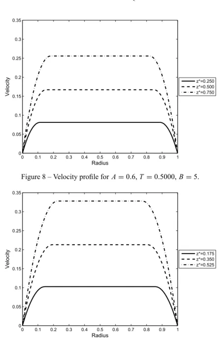
The velocity profiles along radial direction can be obtained by substituting the values ofr∗,h∗,z∗,A,T in the above equations.
Non-dimensionalising equation (23), and integrating it using the boundary conditions, we obtain the following expression for pressure distribution:
P−Pa =
r∗
1
−
12r∗AsinT
(H∗)3−3(1+AcosT)2H∗+2(1+AcosT)3
dr∗ − r∗ 1 ℜ
r∗AcosT
2(1+AcosT)
dr∗−
r∗
1
ℜ
r∗(AsinT)2
20(1+AcosT)
Ŵdr∗
(34)
where
Ŵ≡Ŵ(H∗,H∗′,A,T,r∗)
=
63H∗2+198(1+AcosT)H∗+144(1+AcosT)2−21r∗H∗H∗′−6r∗(1+AcosT)H∗′
(H∗+2(1+AcosT))3
(35)
and
H∗′= 2AsinT H
∗
B
(H∗)2− (1+AcosT)2+2r∗AsinT
B
(36)
The pressure distribution of the squeeze film bearing can be determined for different values of Bingham number, squeeze Reynolds number, amplitude and time by integrating equation (34) numerically.
The load capacity of the circular squeeze film bearing is then given by,
W =
1
0
The integral in equation (37) can be evaluated numerically, for various values of squeeze Reynolds number, amplitude, time and for materials with different values of Bingham number.
4 Results and Discussion
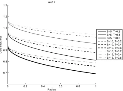
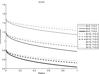
The behavior of core thickness (H∗) for various values of amplitude (A), time (T) and non-Newtonian characteristics (B) at every point of radius (r∗) is computed and the results are given in Figs. 3-6. The core thickness is maximum at the center of the plates and decreases towards the periphery. The core formation decreases with the increase of time for a constant Bingham number and amplitude. Further, it has been found that the thickness of the core increases when the Bingham number increases for a constant time value and amplitude.
0 0.2 0.4 0.6 0.8 1
0.7 0.8 0.9 1 1.1 1.2 1.3
Radius
C
o
re
t
h
ickn
e
ss
A=0.2
B=5, T=0.2 B=5, T=0.4 B=5, T=0.6 B=10, T=0.2 B=10, T=0.4 B=10, T=0.6 B=15, T=0.2 B=15, T=0.4 B=15, T=0.6
Figure 3 – Core thickness variation along the radius for A=0.2.
The velocity profiles along the radial direction(r∗)have been plotted for var-ious values along the axial direction(z∗
0 0.2 0.4 0.6 0.8 1 0.5
0.6 0.7 0.8 0.9 1 1.1 1.2 1.3 1.4
Radius
C
o
re
t
h
ickn
e
ss
A=0.4
B=5, T=0.2 B=5, T=0.4 B=5, T=0.6 B=10, T=0.2 B=10, T=0.4 B=10, T=0.6 B=15, T=0.2 B=15, T=0.4 B=15, T=0.6
Figure 4 – Core thickness variation along the radius for A=0.4.
0 0.2 0.4 0.6 0.8 1
0.4 0.6 0.8 1 1.2 1.4 1.6 1.8
Radius
C
o
re
t
h
ickn
e
ss
A=0.6
B=5, T=0.2 B=5, T=0.4 B=5, T=0.6 B=10, T=0.2 B=10, T=0.4 B=10, T=0.6 B=15, T=0.2 B=15, T=0.4 B=15, T=0.6
Figure 5 – Core thickness variation along the radius for A=0.6.
0 0.2 0.4 0.6 0.8 1 0.2
0.4 0.6 0.8 1 1.2 1.4 1.6 1.8
Radius
C
o
re
t
h
ickn
e
ss
A=0.8
B=5, T=0.2 B=5, T=0.4 B=5, T=0.6 B=10, T=0.2 B=10, T=0.4 B=10, T=0.6 B=15, T=0.2 B=15, T=0.4 B=15, T=0.6
Figure 6 – Core thickness variation along the radius for A=0.8.
0 0.1 0.2 0.3 0.4 0.5 0.6 0.7 0.8 0.9 1 0
0.02 0.04 0.06 0.08 0.1 0.12 0.14 0.16 0.18
Radius
Ve
lo
ci
ty z*=0.325
z*=0.650 z*=0.975
Figure 7 – Velocity profile forA=0.6,T =0.3333,B=5.
0 0.1 0.2 0.3 0.4 0.5 0.6 0.7 0.8 0.9 1 0
0.05 0.1 0.15 0.2 0.25 0.3 0.35
Radius
Ve
lo
ci
ty z*=0.250
z*=0.500 z*=0.750
Figure 8 – Velocity profile forA=0.6,T =0.5000,B=5.
0 0.1 0.2 0.3 0.4 0.5 0.6 0.7 0.8 0.9 1 0
0.05 0.1 0.15 0.2 0.25 0.3 0.35
Radius
Ve
lo
ci
ty z*=0.175
z*=0.350 z*=0.525
Figure 9 – Velocity profile forA=0.6,T =0.6667,B=5.
0 0.1 0.2 0.3 0.4 0.5 0.6 0.7 0.8 0.9 1 0
0.05 0.1 0.15 0.2 0.25 0.3 0.35
Radius
Ve
lo
ci
ty z*=0.175
z*=0.350 z*=0.525
Figure 10 – Velocity profile for A=0.6,T =0.6667,B=10.
0 0.1 0.2 0.3 0.4 0.5 0.6 0.7 0.8 0.9 1 0
0.05 0.1 0.15 0.2 0.25 0.3 0.35
Radius
Ve
lo
ci
ty z*=0.175
z*=0.350 z*=0.525
Figure 11 – Velocity profile for A=0.6,T =0.6667,B=15.
charac-0 0.2 0.4 0.6 0.8 1 1
2 3 4 5 6 7 8
B=5, Re=0 B=10, Re=0 B=15, Re=0 B=5, Re=10 B=10, Re=10 B=15, Re=10 B=5, Re=20 B=10, Re=20 B=15, Re=20
Figure 12 – Load capacity variation with time forA=0.2.
0 0.2 0.4 0.6 0.8 1
1 2 3 4 5 6 7 8 9 10 11
B=5, Re=0 B=10, Re=0 B=15, Re=0 B=5, Re=10 B=10, Re=10 B=15, Re=10 B=5, Re=20 B=10, Re=20 B=15, Re=20
Figure 13 – Load capacity variation with time forA=0.4.
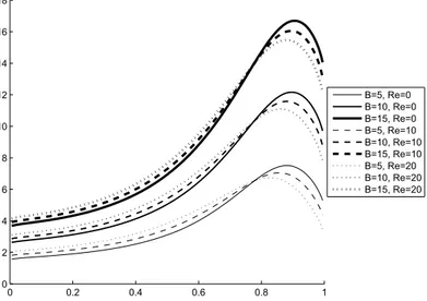
teristics on the load capacity are more significant as the amplitude of the squeeze motion increases.
0 0.2 0.4 0.6 0.8 1 0
2 4 6 8 10 12 14 16 18
B=5, Re=0 B=10, Re=0 B=15, Re=0 B=5, Re=10 B=10, Re=10 B=15, Re=10 B=5, Re=20 B=10, Re=20 B=15, Re=20
Figure 14 – Load capacity variation with time forA=0.6.
0 0.2 0.4 0.6 0.8 1
0 5 10 15 20 25 30 35 40 45
B=5, Re=0 B=10, Re=0 B=15, Re=0 B=5, Re=10 B=10, Re=10 B=15, Re=10 B=5, Re=20 B=10, Re=20 B=15, Re=20
Figure 15 – Load capacity variation with time forA=0.8.
Acknowledgement. The authors would like to thank the reviewers for their valuable comments.
REFERENCES
[2] G.H. Covey and B.R. Stanmore,Use of parallel-plate plastomer for the characterization of viscous study with a yield stress. J. Non-Newtonian Fluid Mech.,8(1981), 249–260.
[3] A.F. Elkouh,Fluid inertia effects in non-Newtonian squeeze films. ASME Trans. J. Lub. Tech.,98(1976), 409–411.
[4] D.K. Gartling and N. Phan-Thien,A numerical simulation of a plastic flow fluid in a parallel plate plastomer. J. Non-Newtonian Fluid Mech.,14(1984), 347–360.
[5] H. Hashimoto and S. Wada,The effects of Fluid Inertia Forces in Squeeze Film Bearings Lubricated with Pseudo-plastic Fluids. Bulletin of JSME,29(1986), 1913–1918.
[6] D.C. Huang, B.C. Liu and T.Q. Jiang,An analytical solution of radial flow of a Bingham fluid between two fixed circular disks. J. Non-Newtonian Fluid Mech.,26(1987), 143–148.
[7] E.J. O’Donovan and R.I. Tanner,Numerical study of the Bingham Squeeze film problem. J. Non-Newtonian Fluid Mech.,15(1984), 75–83.
[8] J.A. Tichy and W.O. Winer,Inertial considerations in parallel circular Squeeze film bearings. ASME Trans. J. Lub. Tech.,92(4) (1970), 588–592.
[9] R. Usha and P. Vimala,Inertia effects in circular squeeze films containing a central air bubble. Fluid Dynamics Research,26(2000), 149–155.