Atmos. Chem. Phys., 12, 3761–3782, 2012 www.atmos-chem-phys.net/12/3761/2012/ doi:10.5194/acp-12-3761-2012
© Author(s) 2012. CC Attribution 3.0 License.
Atmospheric
Chemistry
and Physics
Variability of aerosol, gaseous pollutants and meteorological
characteristics associated with changes in air mass origin at
the SW Atlantic coast of Iberia
J.-M. Diesch1, F. Drewnick1, S. R. Zorn1,*, S.-L. von der Weiden-Reinm ¨uller1, M. Martinez2, and S. Borrmann1,3
1Particle Chemistry Department, Max Planck Institute for Chemistry, Mainz, Germany 2Atmospheric Chemistry Department, Max Planck Institute for Chemistry, Mainz, Germany 3Institute for Atmospheric Physics, Johannes Gutenberg University Mainz, Mainz, Germany *now at: AeroMegt GmbH, Hilden, Germany
Correspondence to:J.-M. Diesch (j.diesch@mpic.de), F. Drewnick (frank.drewnick@mpic.de) Received: 28 September 2011 – Published in Atmos. Chem. Phys. Discuss.: 2 December 2011 Revised: 24 February 2012 – Accepted: 29 March 2012 – Published: 25 April 2012
Abstract. Measurements of the ambient aerosol were per-formed at the Southern coast of Spain, within the frame-work of the DOMINO (DielOxidant MechanismsIn rela-tion toNitrogenOxides) project. The field campaign took place from 20 November until 9 December 2008 at the at-mospheric research station “El Arenosillo” (37◦5′47.76′′N, 6◦44′6.94′′W). As the monitoring station is located at the interface between a natural park, industrial cities (Huelva, Seville) and the Atlantic Ocean, a variety of physical and chemical parameters of aerosols and gas phase could be char-acterized in dependency on the origin of air masses. Back-wards trajectories were examined and compared with local meteorology to classify characteristic air mass types for sev-eral source regions. Aerosol number and mass as well as polycyclic aromatic hydrocarbons and black carbon concen-trations were measured in PM1 and size distributions were
registered covering a size range from 7 nm up to 32 µm. The chemical composition of the non-refractory submicron aerosol (NR-PM1) was measured by means of an Aerosol
Mass Spectrometer (Aerodyne HR-ToF-AMS). Gas phase analyzers monitored various trace gases (O3, SO2, NO, NO2,
CO2) and a weather station provided meteorological
param-eters.
Lowest average submicron particle mass and number con-centrations were found in air masses arriving from the At-lantic Ocean with values around 2 µg m−3 and 1000 cm−3.
These mass concentrations were about two to four times lower than the values recorded in air masses of continental
and urban origins. For some species PM1-fractions in marine
air were significantly larger than in air masses originating from Huelva, a closely located city with extensive industrial activities. The largest fraction of sulfate (54 %) was detected in marine air masses and was to a high degree not neutral-ized. In addition, small concentrations of methanesulfonic acid (MSA), a product of biogenic dimethyl sulfate (DMS) emissions, could be identified in the particle phase.
In all air masses passing the continent the organic aerosol fraction dominated the total NR-PM1. For this reason,
using Positive Matrix Factorization (PMF) four organic aerosol (OA) classes that can be associated with various aerosol sources and components were identified: a highly-oxygenated OA is the major component (43 % OA) while semi-volatile OA accounts for 23 %. A hydrocarbon-like OA mainly resulting from industries, traffic and shipping emis-sions as well as particles from wood burning emisemis-sions also contribute to total OA and depend on the air mass origin.
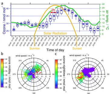
A significant variability of ozone was observed that de-pends on the impact of different air mass types and solar ra-diation.
1 Introduction
Studying tropospheric aerosols is becoming increasingly im-portant as they influence the Earth’s climate (IPCC, 2007), continental, urban and marine ecosystems and visibility
3762 J.-M. Diesch et al.: Variability of aerosol, gaseous pollutants and meteorological characteristics
(Querol et al., 2009). In addition they can have a significant influence on human health (Pope and Dockery, 2006). To study the influence of natural and anthropogenic pollutants emitted by local and regional sources, measurement cam-paigns at remote sites are required where the complex mix-ture of components in the atmosphere can be observed. This mixture depends on the various source regions influencing the measurement site as well as their distance, since chem-ical and physchem-ical processing takes place in an air mass dur-ing transport. In addition, particularly in Southern Europe, the season plays an important role. In the summer months African dust outbreaks, re-circulation of air masses, strong photochemistry and long range transport from NW Europe or Western Iberia (Sanchez de la Campa et al., 2007; Pey et al., 2008) affect the atmospheric composition and levels. The SW of Spain lies next to the Atlantic Ocean and the Strait of Gibraltar, a major ship route. There are several large towns and cities, the largest of them Seville, important ports like the one of Huelva, as well as large agricultural plantations and forests.
The air quality close to the heavily industrialized area around the city of Huelva is significantly degraded at times. Epidemiological studies (CSIC, 2002) as well as the distri-bution of cancer incidents in Spain (Benach et al., 2003) sug-gest that certain kinds of cancers (e.g. lung cancer) occur in this region at an elevated rate. Therefore, a number of stud-ies were performed, mainly in and around Huelva to evaluate the impact of industrial emissions and their characterization in terms of the chemical composition and potential origin (Fern´andez-Camacho et al., 2010b; de la Rosa et al., 2010; Perez-Lopez et al., 2010; de la Campa et al., 2011; Toledano et al., 2009). In addition, the interaction of high solar ra-diation levels as they occur in Andalusia together with ele-vated anthropogenic and natural ozone precursor emissions lead to enhanced photochemical ozone production that can be measured downwind of industrialized regions, where the ozone precursor substances are emitted (Adame et al., 2008, 2010a, b).
So far no comprehensive studies investigating the chem-ical composition of aerosol particles in conjunction with measurements of a variety of trace gases were conducted in Southern Spain. The aim of this study is to present a detailed investigation of the variability of aerosol, trace gas character-istics and meteorological conditions depending on continen-tal, urban and marine sources surrounding the measurement site in “El Arenosillo”. Backwards trajectories were calcu-lated and compared to local meteorology to classify different air mass categories. The non-refractory submicron aerosol composition was determined depending on the air mass cat-egories. The sulfate fraction was further investigated regard-ing aerosol acidity for the individual air mass types. A focus is also on organic components of the aerosol, their sources and variations. Furthermore, the dependence of the diurnal ozone variation associated with meteorological conditions and different air masses was analyzed.
Atlantic
Ocean
Doñana National Park
El
Arenosillo
Seville
Huelva
N
6°W
37°N
0 10 20 km A-494
E-1
A-483 N-435
i
P
o
rtugal
Spain
Morocco
35°N40°N 45°N
8°W 4°W
El Arenosillo
0 2 4 6 8
2 4 6 8
N
E
S W
SE SW
NW NE
a
c
b
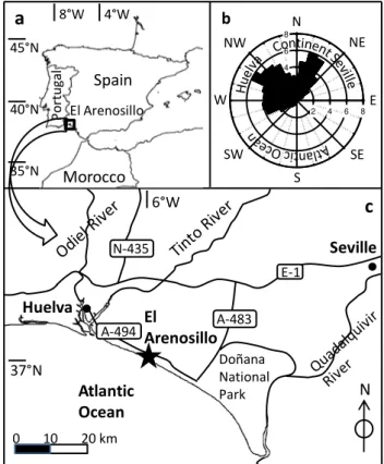
Fig. 1.Map of Spain(a)showing the location of the field measure-ments(c)and an angular histogram of the wind directions recorded during the campaign(b).
2 Overview of the 2008 DOMINO campaign
The 2008 DOMINO (Diel Oxidant Mechanisms In rela-tion toNitrogenOxides) research campaign took place from 20 November until 9 December at the atmospheric research station “El Arenosillo” (37◦5′47.76′′N, 6◦44′6.94′′W) in the southwest of Spain (Fig. 1a), operated by the INTA (Na-tional Institute for Aerospace Technology). The main ob-jective of the campaign was to characterize the oxidative ca-pacity of the troposphere. For this reason, the focus was to study the atmospheric oxidation chemistry, to compare the radical and nighttime chemistry and to characterize the self-cleaning efficiency of the atmosphere in different air mass types. Our contribution to this project was the investigation of the aerosol particle chemistry, composition, formation and transformation processes. Therefore, we measured a large number of atmospheric parameters simultaneously.
The “El Arenosillo” research station lies within a Pro-tected Natural Area in between 3 very different source re-gions: the Atlantic Ocean, the town of Huelva (20 km dis-tance) and the nearby National Park of Do˜nana. The At-lantic Ocean itself has relatively low levels of pollutants, however there are shipping emissions from heavy ship traf-fic in the Strait of Gibraltar (Pey et al., 2008). Huelva is a highly industrialized town with three large chemical estates
J.-M. Diesch et al.: Variability of aerosol, gaseous pollutants and meteorological characteristics 3763
where fertilizer production industries, petrochemical indus-tries, ammonia and urea industries as well as paper produc-tion industries are situated (Carretero et al., 2005; Alastuey et al., 2006; Querol et al., 2002, 2004; Fern´andez-Camacho et al., 2010a). The nearby National Park of Do˜nana on the other hand is a Nature Preserve Park with a large variety of ecosystems and a unique biodiversity (de la Campa et al., 2009). Situated in the west of the Guadalquivir River, it is a UNESCO Biosphere Reserve and Heritage of Mankind consisting of marshlands, pine forests, preserves and mov-ing sand dunes. Beyond it at 70 km distance from the site lies the city of Seville, the capital of Andalusia (population: 704 000). However it is less industrialized than Huelva (pop-ulation: 149 000) which is located at the southwestern end of the Andalusian region and is surrounded by the rivers Odiel and Tinto and the Atlantic Ocean (Fig. 1c). The predomi-nant wind directions at the station during the time the study took place were WSW, NW and NNE transporting air from Seville, Huelva, the Continent and the Atlantic Ocean to the measurement site (Fig. 1b).
In order to study the variability of the particle loading, composition, size distributions as well as trace gas and mete-orological parameters in different types of air masses whose origin is well defined, the campaign was conducted in winter. This offers the advantage to achieve a better understanding of the characteristics, sources and processes, as typical sum-mer features in this part of Southern Europe are reduced: en-hanced photochemistry or recirculation periods that typically occur in spring and summer seasons in this part of Southern Europe (Pey et al., 2008) would contribute to a more complex study scenario.
In the beginning of the campaign from 20 November un-til 3 December fair weather conditions with sunny days and clear skies prevailed. Therefore, a stable nocturnal boundary layer existed and low altitude emissions for example from Huelva were accumulated and measured at elevated concen-trations. Only on two nights (28–29 and 29–30 November) short precipitation periods occurred which did not change the atmospheric composition significantly as the wind originated from the marine source region and concentrations remained as low as before. During the last 6 days of the campaign (3–9 December), it was cloudy with nearly constant temperature, relative humidity and air pressure near ground.
2.1 Setup for ground based measurements of aerosol, gas phase species and meteorology
2.1.1 Key instrumentation
Measurements of the ambient aerosol and several trace gas concentrations were performed using MoLa, a mobile plat-form for aerosol research (Drewnick et al., 2012). During this campaign physical aerosol particle properties in PM1
were detected by the ultrafine water-based Condensation Par-ticle Counter in the 5 nm to 3 µm size range (CPC 3786, TSI,
Inc.) as well as the Filter Dynamics Measurement System Tapered Element Oscillating Microbalance (FDMS-TEOM, Rupprecht & Patashnick Co., Inc.) (see Table 1). For par-ticle size information, a Fast Mobility Parpar-ticle Sizer (FMPS 3091, TSI, Inc.), an Aerodynamic Particle Sizer (APS 3321, TSI, Inc.) as well as an Optical Particle Counter (OPC 1.109, Grimm) were used to cover a particle size range from 7 nm until 32 µm. The chemical composition of the non-refractory (NR) aerosol in the submicron range was measured by means of a High-Resolution Time-of-Flight Aerosol Mass Spectrometer using the “V-mode” (HR-ToF-AMS, Aerodyne Res., Inc.). The black carbon concentration in PM1was determined by a Multi Angle Absorption
Pho-tometer (MAAP, Thermo E.C.) and polycyclic aromatic hy-drocarbons on particles were appointed by the PAH-Monitor (PAS 2000, EcoChem. Analytics). MoLa is also equipped with two instruments to detect various trace gases. An Air-pointer (Recordum GmbH) measures the gas phase species SO2, CO, NO, NO2 and O3. CO2 and H2O were
moni-tored using a LICOR 840 gas analyzer (LI-COR, Inc.). A weather station (WXT 510, Vaisala) provided the most im-portant weather parameters, such as ambient temperature, relative humidity, air pressure, wind speed, wind direction and rain intensity.
2.1.2 Sampling setup
During the field campaign the roof inlet of MoLa, which is normally available for stationary measurements, was used. Next to the roof inlet an extendable mast with the meteo-rological station was fixed, both for measurements in 10 m height. Short branches were used to connect several instru-ments with the main inlet system. The sampling line is op-timized for a flow rate of about 90 l min−1and therefore a pump with flow control was used for regulating this flow in-dependent of the set of instruments operating. The inlet was optimized and characterized for transport losses and sam-pling artifacts (von der Weiden et al., 2009). One of the main characteristics is the occurring aerosol particle loss. Table 1 contains particle loss information for all instruments calcu-lated using theParticle Loss Calculator(von der Weiden et al., 2009). While particle losses have a maximum of 45 % for 20 µm particles for the APS, for all other instruments used during the campaign maximum particle losses are be-low 25 %. The respective losses are relatively small in the size range where the majority of relevant data for this work is collected: in the size range from 30 nm to 2 µm calculated particle losses are below 8 % (without regarding the AMS:
<3 %). Therefore the occurring particle loss can be neglected since they do not influence the measurement results signifi-cantly and the ambient aerosol was measured mostly unbi-ased in this range.
Transport times through the sampling line differ slightly for the individual instruments, so the sampling and measure-ment times are not identical. Therefore the time stamp for
3764 J.-M. Diesch et al.: Variability of aerosol, gaseous pollutants and meteorological characteristics
Table 1. Summary of measured quantities, size ranges and the corresponding particle losses, sampling time delays and detection limits for the instruments implemented in the mobile laboratory (MoLa). Particle losses within the given size range boundaries are lower than those provided here; therefore the given losses are upper limits.
Measurement Instrument
Measured Quantity Size Range/
(Particle losses)
Sampling Delay
Detection Limits/ Accuracy
AMS
Aerosol Mass Spectrometer
size-resolved Aerosol Chemical Composition
40 nm (6 %)– 600 nm (2 %) (vacuum aerodynamic diameter)
43 s sulfate: 0.04 µg m−3 nitrate: 0.02 µg m−3 ammonium: 0.05 µg m−3 chloride: 0.02 µg m−3 organics: 0.09 µg m−3
MAAP
Multi Angle Absorp-tion Photometer
Black Carbon Particle Mass Concentration
10 nm (4 %)– 1 µm (0.2 %)
7 s 0.1 µg m−3
PAH-Sensor
Polycyclic Aromatic Hydrocarbons Sensor
total PAH
Mass Concentration
10 nm (11 %)– 1 µm (0.3 %)
8 s 1 ng m−3
CPC
Condensation Particle Counter
Particle
Number Concentration
5 nm (25 %)– 3 µm (0.8)
7 s N/A
TEOM
Tapered Element Oscillating Microbalance
Particle
Mass Concentration (PM1)
<1 µm (0.5–9 %) 9 s 2.5 µg m−3
FMPS
Fast Mobility Particle Sizer
Particle Size Distribution based on Electrical Mobility
7 nm (9 %)– 523 nm (0.1 %) (Dmob)
7 s N/A
APS
Aerodynamic Particle Sizer
Particle Size Distribution based on Aerodynamic Sizing
0.37 µm (0.1 %)– 20 µm (45 %) (Daero)
7 s N/A
OPC
Optical Particle Counter
Particle Size Distribution based on Light Scattering Cross Section
0.25 µm (0.05 %)– 32 µm (0.002 %) (Dopt)
8 s N/A
Airpointer
O3, SO2, CO and NO, NO2 Mixing Ratio
N/A 6 s O3:<1.0 nmol mol−1
SO2:<1.0 nmol mol−1
CO:<0.08 µmol mol−1
NOx:<2.0 nmol mol−1
LICOR LI840
CO2and H2O Mixing Ratio
N/A 8 s CO2: 1 µmol mol−1
(accuracy)
H2O: 0.01 pmol mol−1
Met. Station
Wind speed and Direction, Temperature, RH, Rain Intensity, Pressure
N/A 0 s N/A
J.-M. Diesch et al.: Variability of aerosol, gaseous pollutants and meteorological characteristics 3765
each instrument has to be corrected depending on the res-idence time of the aerosol in the tube system. The calcu-lated delays for all instruments were subtracted from the time stamps to get the correct sampling time. The sampling delays for the individual instruments are also presented in Table 1. The time resolution used for this analysis was 1 min for all instruments beside the TEOM which generated 15 min data. 2.1.3 Quality assurance for aerosol chemical
composition measurements
For data quality assurance a variety of calibrations of the AMS were performed before and during the campaign. A particle Time-of-Flight calibration was accomplished prior to the campaign, used to convert particle flight times into the corresponding particle diameters. For determination of the instrument background and several distinct instrument pa-rameters, measurements using a high-efficiency particulate air (HEPA) filter as well as a calibration of the Ionization ef-ficiency (IE) of the ion source were conducted once a week. The sensitivity of the detector was monitored permanently and calibrated frequently as well.
A collection efficiency (CE) factor (Huffman et al., 2005) has to be determined to account for the fraction of particles that are not detected as they bounce off the vaporizer be-fore evaporation and to correct for incomplete transmission of particles through the inlet of the instrument. Usually this factor is determined by comparing AMS measurements with results from other instruments or filter measurements. This factor usually ranges between 0.5 (for 50 % particle loss) and 1 (no bounce) and depends mainly on the measurement con-ditions, for example, relative humidity or particle composi-tion. For the DOMINO campaign, a CE factor of 0.5 for the AMS mass concentrations (organics, sulfate, nitrate, ammo-nium and chloride) was used. When using this typical CE factor, the time series of the ToF-AMS mass concentrations summed with the MAAP black carbon mass concentrations show a good agreement with TEOM PM1 mass
concentra-tions (ratio PMAMS+MAAP/PMTEOM=0.97,R2=0.6).
During normal operation, the AMS collected averaged high resolution mass spectra and species-resolved size distri-butions by alternating through the related operation modes, spending 50 % of the sampling time in each mode. The de-tection limits (LOD, Table 1) for each species were evalu-ated on the basis of the method described by Drewnick et al. (2009). They are defined as
LOD=3·√2·σ (I ) (1)
withσ (I )the standard deviation of the background signals
of the respective species.
2.2 Back trajectories and air mass classification
To classify different source regions that are reflected in the aerosol and trace gas composition of the air arriving at
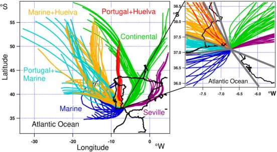
the measurement site, 48 h back trajectories at 10 m arrival height above ground level were calculated for every 2 h dur-ing the whole campaign usdur-ing the HYSPLIT (HYbridSingle Particle Lagrangian Integrated Trajectory) model (Draxler and Rolph, 2003). To analyze the measured data of chemical and physical aerosol particle properties as well as gas phase parameters that are associated with different source regions, the whole dataset was divided according to back trajectories that correspond to similar air mass histories. For this assign-ment we assume that the respective data, one hour before the arrival time and one hour thereafter, “belong” to each tra-jectory and associate these data in the further analysis with the source region defined by the trajectory. Figure 2 shows a map including back trajectories classified into 6 air mass categories based on air mass origins and pathways. The re-sulting air mass categories with the corresponding angles of the limiting trajectory arrival directions as well as the mea-surement time in percent of the entire meamea-surement period are:
– “Seville” (65–82◦, 6 %)
– “Continental” (340–65◦, 15 %) – “Portugal + Huelva” (310–328◦, 3 %) – “Marine + Huelva” (285–310◦, 18 %) – “Portugal + Marine” (265–285◦, 15 %) – “Marine” (140–265◦, 6 %).
To be classified as “Seville”, calculated back trajectories had to cross Seville (latitude and longitude for “Seville” cat-egory borders: 37◦16′11′′N, 5◦54′33′′W and 37◦24′55′′N,
6◦5′1′′W) before approaching the measurement site. Air
masses labeled as “Continental” contain air transported from Spanish inland areas over pine and eucalyptus forests to the station. While “Portugal + Huelva” trajectories mainly travel over Portugal before passing Huelva and then the site; trajectories corresponding to “Marine + Huelva” firstly travelled over the Atlantic Ocean (Huelva category borders: 37◦19′1′′N, 6◦50′36′′W and the coastline). In contrast to “Portugal + Huelva” air masses with trajectories spreading preferentially over the northern part of Huelva city, “Ma-rine + Huelva” trajectories extend over the whole area of the city. Finally, the fifth (“Portugal + Marine”) and sixth (“Ma-rine”) category include marine influenced air masses with the difference that “Portugal + Marine” trajectories also passed Portugal. For each air mass type aerosol as well as gas phase and meteorological parameters were analyzed separately. In total, 63 % of the measured data were considered in our ex-aminations. The remaining data are associated with trajec-tories that passed along the boundaries of the categories and cannot reliably be associated with any of the six categories.
HYSPLIT is intended for transport processes on larger spatial scales due to its relatively low grid resolution. Es-pecially for lower trajectory altitudes, the model suffers
3766 J.-M. Diesch et al.: Variability of aerosol, gaseous pollutants and meteorological characteristics
55
50
45
40
35
-30 -20 -10 0
Seville Continental Portugal+Huelva
Marine+Huelva
Portugal+ Marine
Marine
Atlantic Ocean
Lati
tude
Longitude °S
°W 38.5
38.0
37.5
37.0
36.5
36.0 °S
-7.5 -7.0 -6.5 -6.0 °W
Atlantic Ocean
Fig. 2. On the left side, a map of the Iberian Peninsula is shown including 48 h backwards trajectories calculated for every 2 h using HYSPLIT. The zoom-in at the right shows the transport direction of the classified air mass types at the measurement site. 6 air mass categories corresponding to different source regions were separated: “Seville” (purple), “Continental” (green), “Portugal + Huelva” (red), “Marine + Huelva” (orange), “Portugal + Marine” (light blue), “Marine” (blue).
from severe limitations. Therefore, under the influence of mesoscale processes, HYSPLIT is not able to reproduce lo-cal meteorology adequately. However, during the DOMINO campaign synoptic conditions dominated also regional trans-port which can therefore be reproduced sufficiently accurate down to the lower boundary layer by HYSPLIT calculations as was shown by thorough sensitivity analyses and compar-ison to measurement data (J. A. Adame Carnero, personal communication, 2012).
As a second approach for the identification of the air mass origin, local meteorology was used and measured at the sam-pling site. Here the whole measured data set was divided into different sectors according to the wind direction registered by the meteorological station in 10 m height. In order to avoid associating stagnant air masses with potential contamination from local sources with individual source sectors, all data measured during times with wind speeds below 1 m s−1were not used for further processing. Hereafter, 3 different source regions associated with individual wind directions were iden-tified, called “Continental”, “Urban” and “Marine”.
In Fig. 3 locally measured wind direction data were com-pared for both classification methods. The three differ-ent wind direction ranges of the “Contindiffer-ental” (340–110◦),
“Urban” (285–330◦) and “Marine” (140–265◦) sectors are
shown as grey shaded areas. Red colored box plots reflect the local wind directions measured during the arrival times of the back trajectories associated with various air mass cat-egories. For the “Seville”, “Continental”, “Marine + Huelva” and “Marine” air mass categories, the measured wind direc-tions agree quite well with the wind sectors associated with the same source regions. Contrary, measured wind
direc-350
300
250
200
150
100
50
0
-50
-100
wind direction in degrees
Seville Continental P+Huelva M+Huelva P+Marine Marine
Urban Marine
Continental
Fig. 3.Comparison of wind directions associated with the classified air mass categories (HYSPLIT) with wind direction ranges used for the identification of the three sectors. The wind directions associ-ated with the HYSPLIT air mass categories are presented as box plots (blue marker: mean, box: 25–75 % percentiles with median, whiskers: 5 % and 95 % percentiles) while the wind direction ranges are shown as grey shaded area.
tions of the “Portugal + Marine” air masses are not located within any of the wind direction ranges, because this air mass type could not be separated using the wind direction method, since a gap had to be selected between land (Huelva) and marine influenced air masses. For the “Portugal + Huelva” and “Marine + Huelva” air mass categories the directions of the trajectories differ slightly but systematically from locally measured wind directions, because registered wind direc-tions are influenced by the land-sea-circulation. This effect results in wind directions measured at the site, which was lo-cated directly at the shore, oriented further south – compared to the direction of the trajectories – during daytime while during the night they are rotated more towards the north.
J.-M. Diesch et al.: Variability of aerosol, gaseous pollutants and meteorological characteristics 3767
300
200
100
0
wi
nd dir. / °
-1
21.11.2008 25.11.2008 29.11.2008 03.12.2008 07.12.2008 Date&Time [UTC]
150x103
100
50
0
numbe
r
c
o
n
c
. /
c
m
-3
3.0 2.0 1.0 0.0
BC / µ
g m
-3
20 15
10 5 0
PM
1 /
µ
g
m
-3
50 40 30 20 10 0
o
z
one
/ pp
bv
-1 20
15 10 5 0
SO
2 / ppbv
20 15 10 5 0
NO
x
/ pp
bv
15 10 5 0
m
a
ss c
onc.
/ µ
g m
-3
6 4 2 0
mass conc
.
/
µ
g
m
-3
organics sulfate nitrate
ammonium
chloride
OOAI OOAII
WBOA
HOA
Sev ille
Con tinen
tal
P+H uelv
a
M+H uelv
a
P+M arin
e
Mar ine
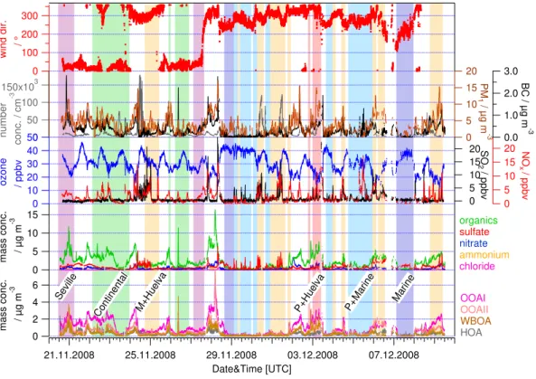
Fig. 4.Time series of several parameters (wind direction (red), number (grey) and PM1mass (brown) concentrations, black carbon (black),
ozone (blue), sulfur dioxide (SO2, black), nitrogen oxide (NOx, red), AMS species (organics (green), sulfate (red), nitrate (blue), ammonium
(orange), chloride (purple), OOAI (purple), OOAII (salmon), WBOA (brown), HOA (grey)) measured during the DOMINO campaign and discussed in the paper. The classified air mass categories are indicated as shaded areas behind the traces (“Seville” (purple), “Continental” (green), “Portugal + Huelva” (red), “Marine + Huelva” (orange), “Portugal + Marine” (light blue), “Marine” (blue)).
In summary, the classification of air mass types made on the basis of back trajectories is more robust than that based on wind directions. HYSPLIT enables a more exact appor-tionment of air masses as it considers not only local condi-tions but also regional and long-range transport influences. However, both methods of associating measurement data to source regions provide similar results when regarding both “Huelva”-related air mass categories as “Urban” and the “Seville” and “Continental” air mass categories as “Conti-nental”. Although very similar results are obtained with both methods, the use of HYSPLIT to identify air masses gives the possibility to separate the data into additional air mass types that cannot be identified on the basis of wind directions alone (e.g. “Seville”).
In Fig. 4 time series for several of the measured parame-ters that are discussed below are shown for the whole cam-paign. The time intervals associated with the classified air mass categories are indicated as shaded areas in different colors. As shown in this figure, for the “Continental”, “Ma-rine + Huelva” and “Portugal + Ma“Ma-rine” air mass categories the air mass origin persisted over relatively long periods on several days. Therefore, the influx from other source regions into these air masses is very unlikely. On the other hand, the “Portugal + Huelva” category was registered only for short
time intervals and only on a single day. Therefore, for this air mass category, influx from other source regions by re-circulation of air masses in varying wind fields cannot be ex-cluded, even though the back trajectories do not show any evidence for this effect. The “Seville” category was mea-sured during two approximately half-day long periods on two different days. Significant differences in the measured pa-rameters have been found for the two time intervals because different phases of new particle formation events have been probed during these times. However, even though mixing with “Continental” air masses is likely, the increased con-centrations measured during these two periods, compared to typical “Continental” concentrations, suggest that actual air masses that at least partially passed Seville have been probed here. Generally both “Marine” periods show very similar evolution of the measured time series, characterized by low concentrations over extended time intervals. During the early phase of the first period, increased concentrations of some aerosol parameters could be an indication of re-circulation of continentally influenced air masses. However, also ship emissions could be the cause of these elevated concentra-tions. Land-sea breeze has been identified to slightly twist locally measured wind directions when air is flowing along the coastline. However, its effect seems to be sufficiently
3768 J.-M. Diesch et al.: Variability of aerosol, gaseous pollutants and meteorological characteristics
Table 2.Averaged submicron mass concentrations and fractions of total PM1for the common HR-ToF-AMS species and black carbon within
the categorized air masses. For each category the total time of measurements is listed that are used for the evaluation. For each species, standard deviations are listed as an estimate for the inner-category variability.
Seville Continental P + Huelva M + Huelva P + Marine Marine
26 h 60 h 11 h 75 h 59 h 26 h
AMS-Org µg m−3 3.2±2.2 2.5±1.7 4.2±1.5 1.8±1.3 0.78±0.63 0.46±0.42
% 58 64 61 45 46 27
AMS-SO4 µg m−3 0.88±0.29 0.49±0.27 0.62±0.33 1.1±0.81 0.50±0.44 0.91±0.43
% 16 13 9.0 28 29 54
AMS-NH4 µg m−3 0.35±0.12 0.22±0.11 0.45±0.38 0.43±0.33 0.17±0.15 0.15±0.089
% 6.4 5.6 6.5 11 10 8.8
AMS-NO3 µg m−3 0.46±0.22 0.29±0.18 0.88±0.50 0.38±0.36 0.094±0.078 0.080±0.054
% 8.4 7.4 13 9.5 5.5 4.7
AMS-Chl µg m−3 0.020±0.020 0.016±0.047 0.25±0.55 0.062±0.060 0.023±0.027 0.022±0.024
% 0.36 0.41 3.6 1.6 1.4 1.3
BC µg m−3 0.54±0.43 0.35±0.24 0.5±0.14 0.29±0.23 0.17±0.17 0.050±0.082
% 9.8 9.0 7.2 7.3 10 2.9
Total Conc. µg m−3 5.5±3.3 3.9±2.6 6.9±3.4 4.0±3.1 1.7±1.5 1.7±1.1 TEOM Conc. µg m−3 4.4±2.8 3.3±2.5 6.4±3.6 4.2±2.8 2.1±1.4 2.2±1.4
small to prevent significant mixing of marine and continen-tally influenced air masses in the identified source categories. As also shown in Fig. 4, the highest concentrations observed on 28 November 2011 were not considered in the study due to an air mass change occurring during this time. Trajectories for this time period show a complex path and a trend, mov-ing further to the West from hour to hour. Therefore, they were not classified into one of the categories. A more in-depth analysis of the influence of topography and transport height on trajectory calculations was performed by scientists of INTA (National Institute for Aerospace Technology) and will be published elsewhere.
3 Results
3.1 Aerosol composition of selected air mass categories
3.1.1 PM1concentrations
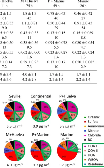
The chemical composition of the submicron aerosol, di-vided into the most common AMS species (organics, sul-fate, nitrate, ammonium, chloride) and black carbon (BC) is presented for each of the air masses in Table 2 and in the pie charts of Fig. 5. Here the total PM1 mass
concen-trations are defined as the sum of all AMS and BC mass concentrations. The lowest average PM1 mass
concentra-tion was found in air masses transported over the Atlantic Ocean (1.7±1.1 µg m−3) (see Table 2). This value was about two to four times lower than the values recorded in air masses of “Continental” (3.9±2.6 µg m−3) and urban (“Huelva”/”Seville”, 4.0±3.1 and 6.9±3.4 µg m−3) ori-gins. Even though the difference in PM1concentrations are
M+Huelva P+Marine Marine
4.0 μg -3 1.7 μg -3 1.7 μg -3
Organic Sulfate Ammonium Nitrate Chloride BC OOA I OOA II HOA WBOA Residuum 24%
14% 11% 10% 16% 8%
6% 0.4%
10%
32%
15% 9% 9% 13% 7%
6% 0.4% 9%
28% 14% 4% 15% 9% 13% 7%
4%7%
19% 14% 6% 6% 28% 10%
11%
2%7%
16% 11% 10% 6% 3% 29% 6%
10%
1%10%
13% 4% 7%
2% 2% 54%
5%9%
1% 3% Seville Continental P+Huelva
5.5 μg -3 3.9 μg -3 6.9 μg -3
Fig. 5.Pie charts of the submicron aerosol composition of the PM1
for each air mass type consisting of organics (green), sulfate (red), ammonium (orange), nitrate (blue), chloride (purple) and black car-bon (black). Organic material was further separated into OOA I (dark purple), OOA II (salmon), HOA (grey) and WBOA (brown) using PMF. The residuum (light blue) cannot be associated with any of these sources or components.
not significant within the one standard deviation boundaries, the trend is clearly evident. Despite the large variability within each category, the values for the air from the Atlantic Ocean largely differ from those of the other two categories. Regarding the whole campaign, total PM1average mass
con-centrations were 4.0±2.5 µg m−3 while black carbon con-tributes 7.9 % (0.32 µg m−3)to this value.
J.-M. Diesch et al.: Variability of aerosol, gaseous pollutants and meteorological characteristics 3769
3.1.2 Particulate organics
Firstly, we note that the organics, sulfate and nitrate NR-PM1
(non-refractory particulate matter with dp≤1 µm) aerosol
concentrations show the most significant levels and also the most contrasting variations dependent on air mass origin. Therefore, they largely determine the chemical character of the aerosol. The highest organic matter fraction (64 %) was measured in the “Continental” air mass category. Biogenic precursor emissions in addition to emissions from frequent biomass burning activities originating from the surrounding pine and eucalyptus forests and the agricultural fields were transported downwind towards the coastal measurement site and generate secondary organic aerosol mass. In addition, anthropogenic sources also result in the generation of organic particulate matter. While the consistently high organic con-tent is the dominant fraction in all air masses that passed the continent, in the “Marine” category sulfate plays the major role. To distinguish between different types of organics and to gain further insights into sources and processes affecting the organic composition results of a factor analysis study are presented in Sect. 3.4.
3.1.3 Non-sea-salt particulate sulfate
Generally, sulfate is a more regionally influenced compo-nent. While in “Continental” influenced air masses 13 % (0.49±0.27 µg m−3) of PM1 consists of “sulfate”, in the
“Marine + Huelva” air mass category a fraction of 28 % (1.1±0.81 µg m−3)was registered. In the marine boundary
layer (MBL) sulfur compounds are quite common (Charlson et al., 1987; Zorn et al., 2008) as the ocean is a large source for atmospheric sulfur (Barnes et al., 2006). In addition, shipping emissions of marine transport in the Strait of Gibral-tar play an important role as reported by Pey et al. (2008). Therefore, “sulfate” is the most abundant species of the “Ma-rine” submicron non-refractory aerosol with a fraction of 54 % (0.91±0.43 µg m−3). The “sulfate” aerosol is further characterized (see Sect. 3.3) by analyzing the acidity since it affects aerosol hygroscopic growth, toxicity and heteroge-neous reactions (Sun et al., 2010).
3.1.4 Particulate nitrate
As a result of a wide variety of industrial and traffic emis-sion sources located in Huelva, nitrate formed by pho-tochemical oxidation of nitrous oxides is the major inor-ganic fraction of the aerosol composition in the “Portu-gal + Huelva” (13 %, 0.88±0.50 µg m−3)air mass category. While in “Marine + Huelva” (9.5 %, 0.38±0.36 µg m−3)and “Seville” (8.4 %, 0.46±0.22 µg m−3)air masses nitrate oc-curs as second most abundant inorganic fraction. It is well known that nitrate is a major content in fine particles from cities, urban and industrial regions (Takami et al., 2005). In addition, source apportionment studies conducted in the
An-dalusian region showed higher average nitrate values in sta-tions with a high traffic influence (de la Rosa et al., 2010). However, ammonium nitrate is volatile and reacts quickly during transport (Takami et al., 2005). The large variabil-ity of concentrations within the air mass categories is caused by the different kinds of emissions from short distances and changing wind directions.
3.1.5 Particulate ammonium
As a major fraction of total inorganic species, nitrate is fol-lowed by ammonium in all air mass types except both “Ma-rine” categories where even less nitrate than ammonium was observed. Nevertheless, ammonium precursor sources in the marine boundary layer (Jickells et al., 2003) are not suffi-ciently abundant to neutralize the present sulfate. For the continentally influenced air masses instead, sources of am-monium include agricultural activities, manures, biomass burning or soils (Bouwman et al., 1997; Hock et al., 2008). The fertilizer production industries in Huelva (Perez-Lopez et al., 2010) provide an increased delivery of ammonia (Car-retero et al., 2005) resulting in highest ammonium concentra-tions in “Portugal + Huelva” (0.45±0.38 µg m−3)and “Ma-rine + Huelva” (0.43±0.33 µg m−3)air masses.
3.1.6 Particulate chloride
The measured chloride content is in the order of 0.4 to 3.6 % within all air masses. However, average chloride val-ues are not dominant in the “Marine” air mass categories as the ToF-AMS cannot measure sea salt (sodium chloride) with significant efficiency (Zorn et al., 2008). In contrast, both “Portugal + Huelva” (3.6 %; 0.25±0.55 µg m−3) and
“Marine + Huelva” (1.6 %, 0.062±0.060 µg m−3)air masses are influenced by industrial emissions (e.g. organic chlo-ride species) likely responsible for up to nine times en-hanced PM1chloride concentrations compared to
“Continen-tal” (0.41 %; 0.016±0.047 µg m−3)air mass types. Low-est chloride values were registered in the “Seville” cate-gory (0.36 %, 0.020±0.020 µg m−3). Since the measured chloride concentrations are either below the detection limit (0.02 µg m−3) or the resulting mass concentrations show large variability, we cannot identify clear differences within the individual source categories for this species.
3.1.7 Black carbon
The influence of air mass histories is also evident in average black carbon (BC) mass concentrations. Enhanced average BC fractions were measured in polluted Huelva (7 %) and “Continental” (9 %) air masses (see Table 2) while lowest BC mass fractions occur in the “Marine” (3 %) influenced air mass category, being typically below the detection limit (0.1 µg m−3). Therefore, an air mass history change leads to a change in measured BC mass concentrations at the site as well.
3770 J.-M. Diesch et al.: Variability of aerosol, gaseous pollutants and meteorological characteristics
40x103
30
20
10
0
number c
onc. / cm
-3
16
12
8
4
0
PM
1
mass conc.
/ µ
g m
-3
Seville Continental P+Huelva M+Huelva P+Marine Marine
AMS+MAAP TEOM
2
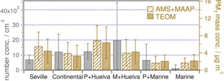
Fig. 6.Averaged particle number (grey) and mass (brown) concen-trations for the individual air mass categories. While hatched brown bars represent averaged submicron PM1mass concentrations
deter-mined by adding HR-ToF-AMS species and black carbon concen-trations, brown filled bars show PM1mass concentrations measured
using the TEOM. Standard deviations show the variability for the mentioned parameters within each air mass category.
3.1.8 Aerosol mass concentrations
Figure 6 illustrates the dependence of average mass con-centrations measured with the TEOM (filled brown) and AMS+MAAP (hatched brown) in PM1 as well as
aver-aged aerosol number concentrations (CPC, grey) on air mass types. Although both mass concentrations are character-ized by large variability (in terms of standard deviations), it is obvious that for all marine influenced source regions TEOM slightly exceeds AMS+MAAP mass concentrations. This is likely due to sea spray which is the major source of particulate matter within the marine boundary layer, consisting of sodium chloride aerosol particles (Warneck, 1988), which cannot be measured efficiently with the AMS. For the “Seville”, “Continental” and “Portugal + Huelva” air mass categories AMS+MAAP concentrations are larger than TEOM mass concentrations. This could be due to volatile substances that are potentially not completely registered us-ing the TEOM.
3.1.9 Particle number concentrations
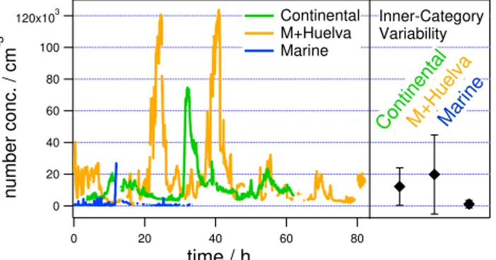
The number concentration levels within the “Continental”, “Marine + Huelva”, “Portugal + Marine” and “Marine” air mass categories show significant variability, reflected in large standard deviations. For the first two of these source sectors the large variability is caused by the frequent occurrence of particle nucleation events. For the “Portugal + Marine” cat-egory particle nucleation is also possible, however, we can neither clearly identify nor exclude such events unambigu-ously. Another potential cause is the inhomogeneous mix-ture of polluted continental air with clean marine air, and for the “Marine” category the generally low values are associ-ated with significant variability, potentially caused by indi-vidual ship emission plumes. Despite the strong variations in number concentrations, a general trend is clearly visible and major differences occur between the group of “Continen-tal”, “Marine + Huelva” and “Portugal + Marine” air masses
compared to the group of “Seville”, “Portugal + Huelva” and “Marine” air masses: the ratios of particle number to particle mass concentration bar heights in Fig. 6 differ significantly between these two groups of air masses. While the brown colored bars corresponding to PM1mass concentrations
re-ferred to the grey ones representing number concentrations are approximately four times as high for the “Marine” cat-egory and 2 times as high for “Seville”, almost the same bar heights were obtained for the “Continental” and “Portu-gal + Marine” air mass categories. The presence of freshly produced aerosol originating from nearby particle sources in “Marine + Huelva” air mass types affect both physical aerosol concentrations in a way that large particle number concentrations associated with lower aerosol mass concen-trations were measured, compared to the other air mass types. On the other hand, the aging of the aerosol during regional transport of urban emissions, like it is the case for “Seville” or aged “Marine” aerosol, is expressed in lower number but enhanced particle mass concentrations. Due to the fact that “Marine + Huelva” air mass trajectories extend over the whole area of Huelva city compared to “Portugal + Huelva”, crossing mainly the north of the city, related concentrations behave differently. Typically, the relation of the particle mass and number concentration shows low correlation (Buonanno et al., 2010). Similar information is provided by the follow-ing particle size distributions with additional details.
3.2 Variability of particle size distributions
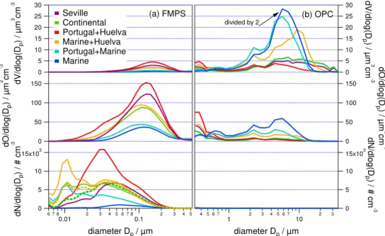
Figure 7 shows the size distributions of averaged number, surface and volume concentrations measured for the different air mass categories using the FMPS (a) and the OPC (b). The FMPS covers the particle size range 7–523 nm (a), whereas the OPC particle size range is from 320 nm until 32 µm (b). The FMPS registers the mobility diameter of the aerosol par-ticles while the OPC measures the optical particle diameter. Since the optical properties of the measured particles are not known well enough, no attempt was made to convert these different particle diameters into a common type of particle diameter. Therefore, both size distributions are shown in sep-arate panels and each mode will be discussed sepsep-arately.
Aging of aerosol particles is often associated with coagu-lation of small particles with each other or onto larger pre-existing particles, and with condensational growth of vapors onto available particle surfaces; resulting in an increase of particle size with time, in a decrease of number concentra-tions and in a change of the particle composition as well. Un-der the condition that particles are larger than 40 nm several hours after particle formation started, e.g. during the growth phase of a nucleation event, changes in particle composition can be investigated using the AMS. However, this topic will be the focus of a future publication.
Within the measured FMPS mobility diameter size range, modes in the averaged number distributions were found in the nuclei mode nearly without exception within all
J.-M. Diesch et al.: Variability of aerosol, gaseous pollutants and meteorological characteristics 3771
Fig.
7
15x103
10
5
0
dN/dl
og(
Dp
) / #
cm
-3
6 7 8 0.01
2 3 4 5 6 7 8
0.1
2 3 4 5
diameter Dp / µm
150
100
50
0
dO
/dlog(D
p
) / µ
m
2 cm
-3
30
25
20 15
10
5
0
dV/dlog(D
p
) /
µ
m
3 cm
-3
Seville Continental Portugal+Huelva Marine+Huelva Portugal+Marine Marine
(a) FMPS
15x103
10
5
0
dN/dlog(D
p) /
#
c
m
-3
4 5 6 7 1
2 3 4 5 6 7
10
2 3
diameter Dp / µm
150
100
50
0
dO/dl
og(
D
p) / µ
m
2
cm
-3
30
25
20 15
10
5
0
dV/dlog(D
p) / µ
m
3
cm
-3
divided by 2 (b) OPC
Fig. 7. Averaged particle size distributions in the size range of 7 nm until 32 µm for all air mass types using the FMPS(a)and OPC(b) data. The FMPS registers particle diameters in a size range of 7–523 nm (Dmob)while the OPC covers the particle size range 320 nm until
32 µm (Dopt). Dotted lines in the number distribution show averaged concentrations without considering new particle formation events for
the “Marine + Huelva” and the “Continental” categories. The observed discrepancies could be due to the fact that both instruments base on different measurement methods and both reach their limits regarding the smallest and largest channels.
continental and Huelva influenced air mass categories. FMPS number size distributions are clearly influenced by frequently occurring particle formation events within these air mass categories. This impact is shown in Fig. 7a using solid and dotted lines of the same color for data where all measurements are considered or where nucleation periods are excluded for the “Continental” and “Marine + Huelva” air mass categories. For the “Portugal + Marine” category we also measured a mode around 10 nm but we can neither identify nor exclude unambiguously new particle formation events for this source category. The significant urban pol-lution in Huelva causes the highest particle number concen-trations for “Portugal + Huelva” including particles in a wide size range with a mode diameter around 30 nm. In Huelva-related air masses, new particles are also formed by nucle-ation. In addition, industrial exhaust gases condense onto pre-existing particles. Nevertheless, as new particle forma-tion will be dealt within a future paper, we will not go further into details here. For the “Marine” air mass category, the monomodal number size distribution with low total number concentrations indicates processed aerosol.
The surface area size distributions (Fig. 7) with accu-mulation mode diameters around 150 nm have a similar monomodal shape for each category except for the “Portu-gal + Huelva” air masses which are five times as high as those from “Marine” air mass types. The extreme urban pollu-tion in Huelva with maximum number concentrapollu-tions in the 30 nm size range result in maximum surface area
concentra-tions and in a fronting of the particle surface area distribution as well.
The volume size distributions measured primarily using the OPC (Fig. 7b) show interesting features in the coarse mode up to 2 µm optical particle diameter. Volume con-centrations of all marine influenced air masses are higher than those originating from “Continental” or urban source regions. While the averaged volume size distributions for “Marine” and “Portugal + Marine” air masses both have their maxima at 5.7 µm and also a similar shape, the “Ma-rine + Huelva” size distribution is clearly shifted towards larger diameters and therefore has its dominant mode around 10 µm. The major particle source in marine enviroments is sea spray therefore sodium chloride particles contribute sig-nificantly to the volume size distributions in “Marine” and “Portugal + Marine” air masses. The “Marine + Huelva” size distribution is affected by both, sea salt particles and parti-cles originating from Huelva’s industries. “Continental” and “Seville” categories have nearly the same volume concentra-tions and shape, but compared to all marine influenced air masses they are shifted towards larger optical particle sizes.
3.3 Variation of the acidity of the submicron aerosol
The aerosol variability between different air mass types was further characterized by analyzing the contributors that in-fluence the aerosols’ acidity, since it has an important im-pact on both, aerosol hygroscopic growth, toxicity as well as
3772 J.-M. Diesch et al.: Variability of aerosol, gaseous pollutants and meteorological characteristics
a
b
0.12
0.10
0.08
0.06
0.04
0.02
0.00
2*su
lfa
te+nitrat
e+ch
lo
ride
/
µ
mo
l m
-3
0.12 0.10 0.08 0.06 0.04 0.02 0.00
ammonium / µmol m-3
acidic
neutralized
alkaline
Seville Continental P+Huelva M+Huelva P+Marine Marine
50x10-3
40
30
20
10
0
H
+ (2
*s
u
lfa
te
+
n
it
ra
te
+
c
hl
or
id
e-a
m
m
o
n
ium
)
/ µ
mol
m
-3
50x10-3
40 30 20 10 0
sulfate / µmol m-3
fully neutralized - (NH4)2SO4
50% (NH4)2SO4
50% NH4HSO4
SO4
2-
as NH4HSO4
SO42- as H2SO4
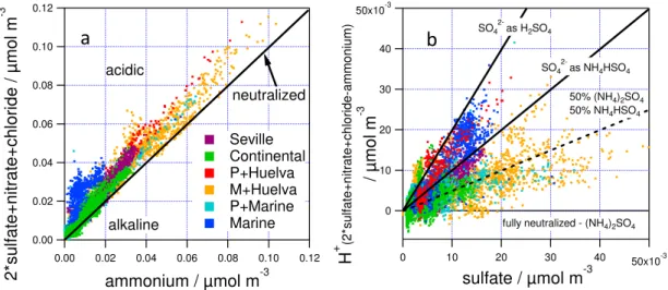
Fig. 8. Correlations illustrating the difference of the ion balance(a)dependent on the air mass origin. The scatter plot(b)serves for the identification of the sulfur species ammonium sulfate ((NH4)2SO4), ammonium bisulfate (NH4HSO4)and sulfuric acid (H2SO4)within the
different aerosols. Points represent 2 min average values.
heterogeneous reactions (Sun et al., 2010). In this context we examined the relative abundance of the inorganic ToF-AMS species sulfate, ammonium and nitrate in the submicron PM1
aerosol, particularly with regard to the differences in the ion balance in dependence of the air mass types.
A scatter plot of the sum of molar sulfate, nitrate and chloride versus molar ammonium is shown in Fig. 8a to il-lustrate the degree of neutralization for the individual air mass classes. Sulfate was multiplied by a factor of 2 to reflect the molar ratio of sulfate versus ammonium in am-monium sulfate. The black line (1:1) indicates fully neu-tralized aerosol. Data points below this line are associ-ated with alkaline aerosol, as ammonium concentrations are higher than needed to neutralize the anions while points lying above this line are associated with acidic aerosol. For most of the points, primarily in “Seville”, “Continental”, “Ma-rine + Huelva” and “Portugal + Ma“Ma-rine” air masses, the cor-relation of measured ammonium versus inorganic anions in-dicates that a major fraction of PM1submicron aerosol was
slightly acidic for most of the time while also neutralized aerosols occur. In “Portugal + Huelva” air masses, the sum of all inorganic AMS anionic compounds (sulfate, nitrate, chlo-ride) exceeds ammonium which implies an acidic aerosol. As mentioned before, acidic sulfate originating from “Marine” air masses measured at this coastal site is due to negligible contribution of ammonium in this region. As shown in the studies of Jickells et al. (2003), ammonium sources are not very abundant in the MBL therefore particulate ammonium concentrations are much smaller than the concentration nec-essary for the neutralization of sulfate and nitrate (Coe et al., 2006; Allan et al., 2004, 2008). Although sodium chloride is the most abundant species in the marine boundary layer, the AMS only measures the NR-PM1aerosol fraction and
there-fore does not measure sodium chloride with significant
effi-ciency (Zorn et al., 2008). For this reason we assume mea-sured chloride is mostly present as ammonium chloride if it is neutralized, hence, it is included in the calculations of the ion balance. Regarding all air mass categories the averaged equivalent ratio is larger than one (see Fig. 8a), indicating that the aerosol at the measurement site was generally rather acidic.
Another focus was put on speciation of sulfur compounds expected to be found in the aerosol from the different source regions. While previous studies in Pittsburgh identified a sul-fur mixture of ammonium sulfate ((NH4)2SO4), ammonium
bisulfate (NH4HSO4)and also small amounts of sulfuric acid
(H2SO4)(Zhang et al., 2007), Zorn et al. (2008) included
the identification and quantification of methanesulfonic acid (MSA) in the analysis, which can be found ubiquitously in marine environments. Figure 8b shows a scatter plot of acid-related hydrogen (H+)present in the particle phase versus
the molar sulfate concentration in the submicron particles. The H+ molar concentration was estimated by subtracting the ammonium (NH+4)molar concentration from the molar concentrations of the anions sulfate (SO24−), nitrate (NO−3)
and chloride (Cl−)(Zhang et al., 2007):
[H+]=2· [SO24−] + [NO−3] + [Cl−]−[NH+4]. (2)
The black lines in Fig. 8b indicate the molar ratios that would correspond to (NH4)2SO4, NH4HSO4 and H2SO4,
the dashed line agrees with 50 % (NH4)2SO4 and 50 %
NH4HSO4. To quantify the various “sulfate” aerosol
compo-nents for the different air mass types in Table 3 the percent-age of ammonium sulfate ((NH4)2SO4), ammonium
bisul-fate (NH4HSO4), sulfuric acid (H2SO4) and
methanesul-fonic acid (MSA) were calculated as follows:
J.-M. Diesch et al.: Variability of aerosol, gaseous pollutants and meteorological characteristics 3773
Table 3. Percentage contribution of ammonium sulfate ((NH4)2SO4), ammonium bisulfate (NH4HSO4), sulfuric acid (H2SO4) and
methanesulfonic acid (MSA) to the species class “sulfate” for the selected air mass categories.
ammonium ammonium sulfuric methanesulfonic
sulfate bisulfate acid acid
% ((NH4)2SO4) (NH4HSO4) (H2SO4) (MSA)
Seville 28 72 0 below LOD
Continental 50 50 0 below LOD
Portugal + Huelva 0 72 28 below LOD
Marine + Huelva 32 68 0 below LOD
Portugal + Marine 26 74 0 below LOD
Marine 0 74 26 1
NH+4excess(mol)= NH+4(mol)−NO−3(mol)−Cl−(mol) (3) SO24−excess(mol)= SO24−(mol)−NH+4excess(mol)/2 (4) %H2SO4= SO24−excess(mol)/SO24−total(mol)·100 (5)
%MSA = MSA(mol)/SO24−total(mol)·100 (6) %(NH4)2SO4= 100−%H2SO4−%MSA. (7)
The fraction of NH4HSO4 for each category can be
cal-culated stoichiometrically based on the molar ratios of (NH4)2SO4and H2SO4.
The “sulfate” classes (NH4)2SO4, NH4HSO4and H2SO4
were distinguished on the basis of the presence of the poten-tial counter ions as we cannot separate the different sulfate species directly in our measurements. Therefore, we assume that ammonium first reacts with nitrate and chloride in the particles and chemical equilibrium exists. Likewise, excess ammonium reacts with sulfate to form ammonium sulfate in an equilibrium reaction. Finally, sulfate that could not be neutralized by ammonium has to be present as ammonium bisulfate or sulfuric acid. In Table 3 the relative contributions of the species (NH4)2SO4, NH4HSO4 and H2SO4 to total
“sulfate” are presented. For calculating MSA concentrations thePeak Integration by Key Analysissoftware (PIKA, http: //cires.colorado.edu/jimenez-group/ToFAMSResources, De-Carlo et al., 2006) was used to deconvolve them/z79 sig-nal into three peaks: Bromine, a MSA fraction, and an or-ganic fragment (C6H+7)as described in Zorn et al. (2008). As
shown in Table 3, the analysis indicates that MSA accounts for only a minor degree (1 %) of the total “sulfate” compo-nent class when “Marine” air masses arrive at the measure-ment site, while MSA concentrations in the other categories are below the detection limit (6 ng m−3).
Unlike in the studies of Zorn et al. (2008) a major frac-tion of the “sulfate” class in the “Marine” air mass category is contributed by ammonium bisulfate (74 %) while sulfuric acid (26 %) is the second major contributor (Fig. 8b). While sulfuric acid is produced from dimethyl sulfide (DMS) orig-inating from phytoplankton or anaerobe bacteria (Charlson et al., 1987) and from sulfur dioxide (SO2)from shipping
emissions (Zorn et al., 2008), ammonium bisulfate is the re-sult of the neutralization reaction between sulfuric acid and
ammonia. In comparison, “Portugal + Huelva” air masses are influenced by nitrate precursor emission sources in Southern Huelva, causing the binding of a significant fraction of the available ammonium. This results in an ammonium bisul-fate (72 %) to sulfuric acid (28 %) ratio that is even more acidic than those within the “Marine” air mass category (Ta-ble 3). On the contrary, ammonia is mostly present in the ter-restrial boundary layer hence sulfurous aerosols are mostly composed of ammonium bisulfate and ammonium sulfate in the “Seville”, “Marine + Huelva” and “Portugal + Marine” air mass types. For the “Continental” air mass category the ammonium sulfate to ammonium bisulfate ratio is balanced. This can also be seen in Fig. 8b based on the corresponding data points reflecting the 50 % (NH4)2SO4/50 % NH4HSO4
line. Similar results were found during the OOMPH cam-paign: Zorn et al. (2008) found only a minor fraction (20– 50 %) of neutralized aerosol during pristine marine domi-nated periods while continentally influenced air masses are often neutralized.
3.4 Factor analysis of the organic aerosol using Positive Matrix Factorization (PMF)
Another major objective of this study is to identify the main components and sources of the submicron organic aerosol. For this purpose positive matrix factorization (PMF) (Paatero, 1997; Paatero and Tapper, 1994) was used to an-alyze the AMS organics information using the evaluation tool developed by Ulbrich et al. (2009). Results of this analysis for the whole campaign period show four “fac-tors”, representing different aerosol types that explain an av-erage of 97 % of the total organic mass and can be associ-ated with aerosol sources and components. Oxygenassoci-ated or-ganic aerosol (OOA I) was the major component that con-tributes on average 43 % of the particulate organic mass dur-ing the whole measurement period. While OOA I, a highly-oxygenated OA, mostly represents secondary organic aerosol (SOA); OOA II, accounting for additional 23 % of the or-ganic mass, represents a less-oxygenated/processed, semi-volatile OA (Ulbrich et al., 2009). A hydrocarbon-like or-ganic aerosol type (HOA, 16 %) as well as aerosol from
3774 J.-M. Diesch et al.: Variability of aerosol, gaseous pollutants and meteorological characteristics O HO H H HO H H OH O
a
b
c
1
2
3
4
1
2
3
4
1
2
3
4
OOA
I
OOA
II
HOA
WBOA
0.20 0.15 0.10 0.05 0.00 OO AI / µ
g m -3 100 90 80 70 60 50 40 30 20 m/z 0.25 0.20 0.15 0.10 0.05 0.00 OO A II / µ g m -3 100 90 80 70 60 50 40 30 20 m/z 0.14 0.12 0.10 0.08 0.06 0.04 0.02 0.00 HO A / µ g m -3 100 90 80 70 60 50 40 30 20 m/z 0.10 0.08 0.06 0.04 0.02 0.00 WBO A / µ g m -3 140 120 100 80 60 40 20 m/z 3.5 3.0 2.5 2.0 1.5 1.0 0.5 0.0 OO A
I / µ
g m -3 4 3 2 1 0 SO4
/ µg m-3
3.5 3.0 2.5 2.0 1.5 1.0 0.5 0.0 OOA
I / µ
g m -3 10 8 6 4 2 0
SO2 / ppbv
3.0 2.5 2.0 1.5 1.0 0.5 0.0 O O AI
I / µ
g m -3 1.5 1.0 0.5 0.0
NO3- / µg m-3
3.0 2.5 2.0 1.5 1.0 0.5 0.0 OO
AII / µ
g m -3 3.60x10⁻³ 3.55 3.50 3.45 3.40
air temp.-1 / k
2.0 1.5 1.0 0.5 0.0 HOA / µ g m -3 1.2 0.8 0.4 0.0
BC / µg m-3
2.0 1.5 1.0 0.5 0.0 HO
A / µ
g m -3 12 10 8 6 4 2 0
NOx / ppb
Seville Continental P+Huelva M+Huelva P+Marine Marine 2.5 2.0 1.5 1.0 0.5 0.0 W B O A / µ g m -3 80x10-3 60 40 20 0
LG m/z 60 / µg m-3
4 3 2 1 0 WB OA / µ g m -3 1.2 0.8 0.4 0.0
BC / µg m-3
3.0 2.5 2.0 1.5 1.0 0.5 0.0
OOAI / µ
g
m
-3
00 01
01 02
02 03
03 04 04
05 05
06 06
07 07
08 08
09 09
10 10
11 11
12 12
13 13
14 14
15 15
16 16
17 17
18 18
19 19
20 20
21 21
22 22
23 23
24
Time of day / UTC
2.0 1.5 1.0 0.5 0.0 OO AI
I / µ
g
m
-3
00 01
01 02
02 03 03
04 04
05 05
06 06
07 07
08 08
09 09
10 10
11 11
12 12
13 13
14 14
15 15
16 16
17 17
18 18
19 19
20 20
21 21
22 22
23 23
24
Time of day / UTC
14 12 10 8 a ir te mp . / ° C 1.2 1.0 0.8 0.6 0.4 0.2 0.0 WB O A / µ g m -3
00 01 01
02 02
03 03
04 04
05 05
06 06
07 07
08 08
09 09
10 10
11 11
12 12
13 13
14 14
15 15
16 16
17 17
18 18
19 19
20 20
21 21
22 22
23 23
24
Time of day / UTC 0.8 0.6 0.4 0.2 0.0 HO A / µ g m -3
00 01
01 02 02
- 03 03
04 04
05 05 - 06
06 - 07
07 08 08
09 09 - 10
10 11
11 12 12
- 13 13 - 14
14 15
15 16 16
- 17 17
18 18
19 19 - 20
20 - 21
21 22 22
23 23 - 24
Time of day / UTC
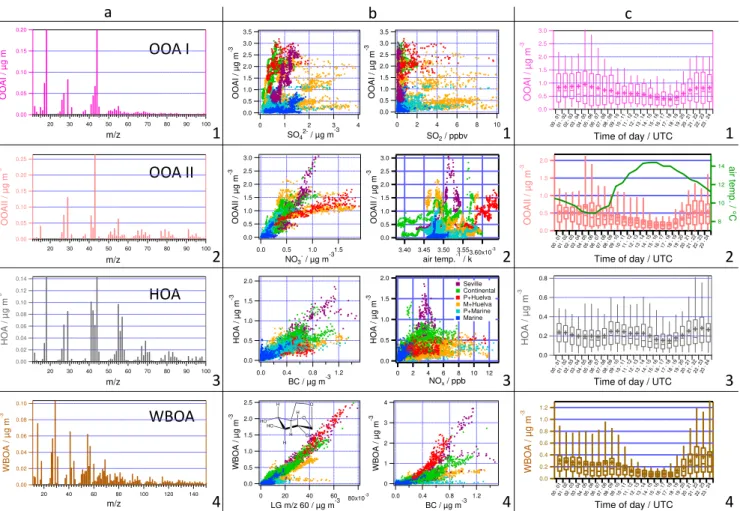
Fig. 9.Mass spectra(a), correlations(b)and diurnal variation box plots(c)of OOA I (dark purple, 1), OOA II (salmon, 2), HOA (grey, 3) and WBOA (brown, 4) organic aerosol types. Mass spectral markers were compared to reference spectra (not shown). The four factors were correlated with aerosol species (sulfate, nitrate,m/z60 as levoglucosan tracer, black carbon), trace gases (nitrogen oxide, sulfur dioxide) and meteorological parameters (air temperature)(b). Box plots of the diurnal variation for the whole campaign(c)show the median, mean and the 25/75 % percentiles. The whiskers indicate the 5/95 % interquartile span. Points in the correlations(b)represent 2 min average values.
wood burning emissions (WBOA, 15 %) were identified in this study by comparing the mass spectra of the PMF factors to measured ambient reference spectra (http://cires.colorado. edu/jimenez-group/AMSsd/).
3.4.1 Comparison of mass spectra with reference spectra
In Fig. 9a calculated average mass spectra of all four PMF factors (OOA I, OOA II, HOA, WBOA) are shown. Sig-nificant mass fragments for highly-aged OOA I (Fig. 9a/1) are m/z 18, 27, 41, 43, 44, 55, 69 while marker peaks at
m/z 27, 29, 41, 43, 55, 67, 79 are characteristic for OOA II (Fig. 9a/2). Both factors correlate well with reference spectra shown in Lanz et al. (2007) (R2=0.96 for OOA I;R2=0.90 for OOA II). Unlike in the studies of Lanz et al. (2007), Zhang et al. (2005) and Ulbrich et al. (2009), the HOA mass spectrum found in this work (Fig. 9a/3) is dom-inated bym/z 44 and thereforem/z 18 and 17 mass
frag-ments are enhanced as well, because their calculation was bound tom/z 44 in the analysis. Apart from this, the typ-ical characteristic peaks for hydrocarbons (m/z 41, 43, 55, 57, 69, 81, 95) exist. Therefore, we assume this factor rep-resents a “slightly oxidized HOA”. For this reason, the HOA reference spectrum (Zhang et al., 2005) does not correlate very well (R2=0.58) with our HOA spectrum. Moreover, regarding the high resolution mass spectra at m/z 44, the C3H+8 peak (m/z44.06) overlaps the CO+2 peak (m/z43.99)
and could not be separated with the AMS as the mass res-olution was too low. Therefore, this could also be a reason for the enhancedm/z44 signal which is not associated with oxidized organic aerosol. In addition a spectral pattern was determined in the fourth factor in this study which is similar to the wood burning reference spectrum in Lanz et al. (2007) (R2=0.83), containing prominent peaks atm/z15, 29, 41, 55, 60, 69, 73, 91 (WBOA, Fig. 9a/4).