HESSD
8, 4789–4811, 2011Effects of seasonality on the distributions
of hydrological extremes
P. Allamano et al.
Title Page
Abstract Introduction
Conclusions References
Tables Figures
◭ ◮
◭ ◮
Back Close
Full Screen / Esc
Printer-friendly Version
Interactive Discussion
Discussion
P
a
per
|
Dis
cussion
P
a
per
|
Discussion
P
a
per
|
Discussio
n
P
a
per
|
Hydrol. Earth Syst. Sci. Discuss., 8, 4789–4811, 2011 www.hydrol-earth-syst-sci-discuss.net/8/4789/2011/ doi:10.5194/hessd-8-4789-2011
© Author(s) 2011. CC Attribution 3.0 License.
Hydrology and Earth System Sciences Discussions
This discussion paper is/has been under review for the journal Hydrology and Earth System Sciences (HESS). Please refer to the corresponding final paper in HESS if available.
E
ff
ects of seasonality on the distribution
of hydrological extremes
P. Allamano, F. Laio, and P. Claps
Politecnico di Torino, Corso Duca degli Abruzzi 24, 10123 Torino, Italy
Received: 10 May 2011 – Accepted: 11 May 2011 – Published: 13 May 2011 Correspondence to: P. Allamano ([email protected])
HESSD
8, 4789–4811, 2011Effects of seasonality on the distributions
of hydrological extremes
P. Allamano et al.
Title Page
Abstract Introduction
Conclusions References
Tables Figures
◭ ◮
◭ ◮
Back Close
Full Screen / Esc
Printer-friendly Version
Interactive Discussion
Discussion
P
a
per
|
Dis
cussion
P
a
per
|
Discussion
P
a
per
|
Discussio
n
P
a
per
|
Abstract
This paper focuses on the seasonality of hydroclimatic extremes and on the problem of accounting for their non-homogeneous character in determining the design value. To this aim we devise a simple stochastic world in which extremes are produced by a non-homogeneous extreme value generation process. The design values are estimated 5
in closed analytical form both in a peak over threshold framework and by using the standard annual maxima approach. In this completely controlled world of generated hydrological extremes, a statistical measure of the error associated to the adoption of a homogeneous model is introduced. The sensitivity of this measure, assumed in terms of return period ratio, to the typology and strength of seasonality is investigated. 10
We find that seasonality induces a downward bias in design value estimators. The magnitude of the bias may be large when the peak over threshold approach is adopted, while the return period distortion is limited when the annual maxima are considered. An application to a prealpine to alpine transition region located in North-Western Italy is presented to better clarify the effects of disregarding seasonality in a real case.
15
1 Introduction
Hydrological variables, like precipitation depth and river discharge, often exhibit marked periodic variability on annual time scales (Black and Werritty, 1996; Sivapalan et al., 2005; Rust et al., 2009; Viglione et al., 2010; Villarini et al., 2011). As a conse-quence, also the corresponding extreme values, i.e. the precipitation or discharge 20
values associated to relevant and unfrequent events, will likely be dependent on the non-homogeneity of their respective date of occurrence. The seasonal variability of ex-treme events represents an issue for the standard applications of the frequency anal-ysis, because in the presence of seasonality the sample values available for design value estimation could belong to different populations. The manner how these
date-25
HESSD
8, 4789–4811, 2011Effects of seasonality on the distributions
of hydrological extremes
P. Allamano et al.
Title Page
Abstract Introduction
Conclusions References
Tables Figures
◭ ◮
◭ ◮
Back Close
Full Screen / Esc
Printer-friendly Version
Interactive Discussion
Discussion
P
a
per
|
Dis
cussion
P
a
per
|
Discussion
P
a
per
|
Discussio
n
P
a
per
|
The standard procedures for design value estimation are based on the analysis of series of annual maxima (AM). Estimation of the distribution of annual maxima from data with seasonal variability has received attention in the literature. Attempts to obtain the annual maximum distribution by fitting different distributions to the maxima in
sepa-rate seasons – and to derive the expressions for the bias and variance of the resulting 5
annual quantile estimators – were done by Lamberti and Pilati (1985) and Buishand and Demar ´e (1990). The basic idea is to have, in each season, random variables that satisfy the “identically distributed” hypothesis, which is essential in standard statisti-cal inference. The use of monthly maxima has also been advocated (e.g., Carter and Challenor, 1981; Ettrick et al., 1987; Rust et al., 2009) because the hypothesis of iden-10
tically distributed random variables in classical extreme-value theory is better satisfied for monthly than for annual maxima. The problem with these approaches is that the number of parameters to be estimated increases, which in turn inflates the estimation uncertainty of design values. Moreover, the application of these methods requires non-standard data (maxima in separate seasons) which are seldom available for long time 15
periods.
An alternative is offered by the peak over threshold (POT) or partial duration series
approach. This approach considers several over-threshold values instead of a unique extreme value per year (Madsen et al., 1997; Lang et al., 1999; Claps and Laio, 2003). The strongest motivation for adopting the POT approach is that monthly or seasonal 20
maxima constitute precious additional information about the upper tail of the distribu-tion, which is very important in hydrological applications (Revfeim, 1991; Katz et al., 2002). The POT approach naturally lends itself to being used with a rate of occurrence of the exceedances (λ) and an exceedances distribution having an annual cycle (Todor-ovic and Zelenhasic, 1970). However, standard applications of the POT approach do 25
not consider time-dependent parameters (e.g., Madsen et al., 1997; Claps and Laio, 2003). The aim of this paper is to provide indications about the effects of neglecting
HESSD
8, 4789–4811, 2011Effects of seasonality on the distributions
of hydrological extremes
P. Allamano et al.
Title Page
Abstract Introduction
Conclusions References
Tables Figures
◭ ◮
◭ ◮
Back Close
Full Screen / Esc
Printer-friendly Version
Interactive Discussion
Discussion
P
a
per
|
Dis
cussion
P
a
per
|
Discussion
P
a
per
|
Discussio
n
P
a
per
|
2 A “toy-model” for understanding seasonality effects on the distributions of
extremes
A simplified analytical model of the distribution of precipitation extremes is devised, in which precipitation is assumed to follow a non-homogeneous Poisson process of storm arrivals in time with rateλ, the depthxof each storm being distributed according to an 5
exponential function
F(x|t)=1−exp[−x/α(t)] (1)
where the meanα(t) of the distribution is dependent on time. Despite its simplicity, the model is widely adopted in hydrology, as demonstrated by the numerous applications that can be found in the literature (e.g., Eagleson, 1978; Rodriguez Iturbe et al., 1987; 10
Rasmussen and Rosbjerg, 1989; Laio et al., 2001). To mimic the effects of seasonality
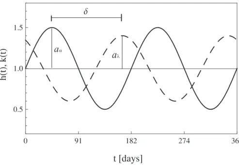
on the precipitation regime, a sinusoidal (time-dependent) variation is imposed on the parameters of the Poisson process. We writeα(t) andλ(t) as
α(t)=α0 1+aαsin 2π
365nt
=
α0·h(t),
λ(t)=λ0 1+aλsin 2π
365nt+δ
=
λ0·k(t),
(2)
where α0 and λ0 are the average rainfall intensity and rainfall rate values; t is time 15
in days (t∈[0;365]); nis the number of peaks per year; h(t) is the non-dimensional
α regime and k(t) the non-dimensional λ regime; aα and aλ are, respectively, the amplitudes of the sinusoids h(t) and k(t); and δ is the temporal shift between the two. Note that, to constrainh(t) andk(t) above zero,aα andaλ can vary in the range
(0,1). Observe also that the initial timet=0 is taken at any point whereα(t)=α0and
20
dα(t)/dt >0. An example for theh(t) andk(t) curves is reported in Fig. 1.
The distribution in Eq. (1) is the conditioned distributionF(x|t) of the rainfall depths
x on the date of occurrencet. The marginal distribution of precipitation exceedances
HESSD
8, 4789–4811, 2011Effects of seasonality on the distributions
of hydrological extremes
P. Allamano et al.
Title Page
Abstract Introduction
Conclusions References
Tables Figures
◭ ◮
◭ ◮
Back Close
Full Screen / Esc
Printer-friendly Version
Interactive Discussion
Discussion
P
a
per
|
Dis
cussion
P
a
per
|
Discussion
P
a
per
|
Discussio
n
P
a
per
|
some further manipulation of Eq. (1) is needed. To this end we approximateF(x|t) in Eq. (1) by
F′(x|t)=1−exp[−x·α′(t)] (3)
withα′(t)=α′
0·h′(t)=α′0(1−a′αsin(nt)). The minus sign before the sine assures that
the maxima and minima ofα0′ anda′α are in phase. The values of the parametersα0′ 5
and a′α should be found which minimize the distance between F′(x|t) and F(x|t). A possible strategy could be to calculate the total squared distance
TSD(α0′,a′α)=
Z365
0
[F(x|t)−F′(x|t)]2dt=
Z365
0
e−2x/α(t)h1−e−x(α′(t)−1/α(t))i2dt (4)
and to find the values ofα0′ and a′α which minimize TSD(α′0,a′α). The solution to this
equation does not provide an analytical result, but one can observe that the integral 10
on the right hand side of Eq. (4) can be seen as a weighted average of the distance between the curves, where the weighting factor isw(t)=e−2x/α(t). It is clear that this
weighting factor is maximum where α(t) is largest, i.e. in t′=365(π/2n+2π/n)/2π
and minimum in t′′=365(3π/2n+2π/n)/2π. The ratio between the minimum and
maximum weighting factors reads 15
r=e
−α0(12x−aα)
e−α0(12x+aα)
=e−
4xaα
α0(1−a2α) (5)
and rapidly converges to zero for large values ofx, which are those of interest in this paper. The differences betweenF′(x|t) andF(x|t) are therefore negligible whenα(t) is
small, and it is sensible to determineα0′ anda′0whenα(t) attains its maximum, i.e. in
t′. By settingt′fort inF(x|t) andF′(x|t) and equating the two expressions one easily 20
obtainsα0′=1/α0anda′α=aα/(1+aα).
HESSD
8, 4789–4811, 2011Effects of seasonality on the distributions
of hydrological extremes
P. Allamano et al.
Title Page Abstract Introduction Conclusions References Tables Figures ◭ ◮ ◭ ◮ Back Close
Full Screen / Esc
Printer-friendly Version Interactive Discussion Discussion P a per | Dis cussion P a per | Discussion P a per | Discussio n P a per | form:
F(x)=
Z365
0
F′(x|t)k(t)dt=1−e−α0x
Φ
0, aα α0(1+aα)x
+aλΦ
1, aα α0(1+aα)x
cos(δ)
(6)
whereΦ[·] is the modified Bessel function of the first kind (Abramowitz and Stegun,
1965, ch.9) and k(t) is as defined in Eq. (2). An important property of F(x) is that its expression does not change by changing the oscillation frequency (parameternin 5
Eq. (2)). Observe also that the mean ofF(x) can be expressed analytically as
µx= α0
aα−(1+aα)
r
1+2aα (1+aα)2−1
aλcos(δ)
aα r
1+2aα
(1+aα)2
. (7)
Moreover, the distribution in Eq. (6) tends to an exponential distribution (also called “base POT distribution”) in the homogeneous case, i.e. whenaα=aλ=0.
The distribution of exceedances Eq. (6) can then be transposed into the correspon-10
dent annual maximum distribution. In fact, despite the non-homogeneity of the process, the standard relationFAM(x)=e−
λ0(1−F(x))
(relating the distribution of exceedances to the distribution of annual maxima, FAM(x)) still holds (e.g., Coles, 2001, p. 131). On this premise, the following expression for the distribution of annual maxima is obtained
FAM(x)=exp
−exp
−αx 0 λ0 Φ
0, aαx α0(1+aα)
+aλΦ
1, aαx α0(1+aα)
cos(δ)
(8) 15
in which α0 plays the role of the scale parameter. Observe that the distribution of maxima becomes a Gumbel distribution (also called “base AM distribution”) whenaα= aλ=0 in Eq. (2). Observe also that for Eq. (8) the mean and standard deviation of the
HESSD
8, 4789–4811, 2011Effects of seasonality on the distributions
of hydrological extremes
P. Allamano et al.
Title Page
Abstract Introduction
Conclusions References
Tables Figures
◭ ◮
◭ ◮
Back Close
Full Screen / Esc
Printer-friendly Version
Interactive Discussion
Discussion
P
a
per
|
Dis
cussion
P
a
per
|
Discussion
P
a
per
|
Discussio
n
P
a
per
|
3 Model application
Ignoring the possible effects of seasonality when adapting a distribution to a set of data
is a rather common simplification, especially when few observations are available. In the following we explore the consequences of such a simplification, as they could affect
the return period estimation both for the distribution of exceedances and the distribution 5
of maxima.
To quantify the error associated to the selection of the wrong (non-seasonal) dis-tribution, we consider theT-year event with the base (non-seasonal) distribution and compute the corresponding return period, T∗, with the correct seasonal distribution. The return period ratio
10
RT= T
T∗ (9)
provides an indication of the magnitude of the underestimation (overestimation) in de-sign values related to neglecting seasonality. In particular, ifRT>1 the adoption of the base distribution corresponds to an underestimation of the real design value.
3.1 Peak over threshold
15
Consider precipitation exceedances to follow the distribution in Eq. (6), having mean
µx as defined by Eq. (7). As anticipated, in the homogeneous caseaα=aλ=0, and
the distribution of exceedances becomes an exponential distribution, called base dis-tribution. The design eventxT(POT)with the base distribution is determined as
xT(POT)=−µxlog
1
λ0T
. (10)
20
Using the seasonal distribution Eq. (6) one finds that the same event xT(POT) has a return period T∗, obtained by setting Eq. (10) for x in Eq. (6), and considering that
λ0T∗=1/(1−F(x (POT)
HESSD
8, 4789–4811, 2011Effects of seasonality on the distributions
of hydrological extremes
P. Allamano et al.
Title Page
Abstract Introduction
Conclusions References
Tables Figures
◭ ◮
◭ ◮
Back Close
Full Screen / Esc
Printer-friendly Version
Interactive Discussion
Discussion
P
a
per
|
Dis
cussion
P
a
per
|
Discussion
P
a
per
|
Discussio
n
P
a
per
|
Given the simplicity of the model the return period ratio is obtained in analytical form, and reads
RT(POT)=λ0T
1
λ0T
z(1 +aα)
aα
Φ
0,zlog
1
λ0T
−aλΦ
1,zlog
1
λ0T
cos(δ)
(11)
withz=[aα−(1+aα)(
q
(1+2aα)/(1+aα)2−1)a
λcos(δ)]/ p
1+2aα. Note that Eq. (11)
is independent of the mean rainfall intensityα0 because α0 is a scale parameter for 5
both the base and the seasonal distribution.
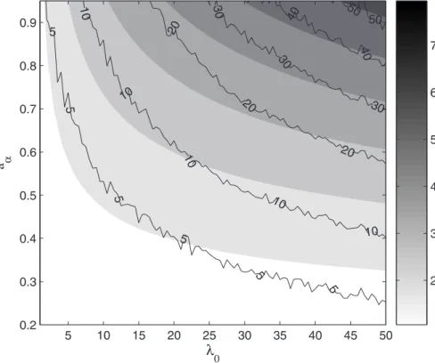
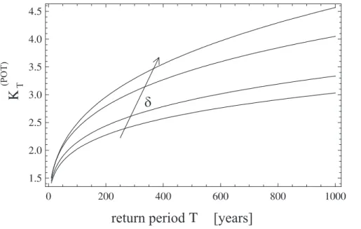
The sensitivity of the return period ratio to the parameters of Eq. (6) is explored in Fig. 2 (gray-shaded contour areas). The results are obtained by varying two param-eters at a time and by fixing the other paramparam-eters. In particular, in Fig. 2,λ0 and aα
are assumed to vary. In each point of the plane the intensity of the grey-shade is pro-10
portional to the value of the return period ratio, with large values of the return period ratio RT(POT) corresponding to precipitation events RT(POT) times more frequent in the “seasonal reality” than if the exponential distribution was adopted. We find a strong sensitivity of the return period ratio to large values ofaα and λ0 (with values that can be as large as 7). The sensitivity ofRT(POT)to the variation of the two other parameters 15
T and δ is shown in Fig. 3: it emerges that RT(POT) significantly increases both with the return periodT and the phase shiftδ. From Fig. 3 it can be deduced thatRT(POT)
assumes slightly lower values when the regimes are in phase, as in the case illustrated in Sect. 4.
One could argue that the difference between the two distributions would be
recog-20
nized if the data were closely scrutinized. This is verified by applying a goodness of fit test for exponentiality to the samples generated by the seasonal model. In details, 1000 samples of lengthN′, generated from the distribution Eq. (6) under different
pa-rameterizations, are tested with the Anderson-Darling test (see Laio, 2004) against the hypothesis of exponential distribution. In Fig. 2, black labelled contour lines show 25
HESSD
8, 4789–4811, 2011Effects of seasonality on the distributions
of hydrological extremes
P. Allamano et al.
Title Page
Abstract Introduction
Conclusions References
Tables Figures
◭ ◮
◭ ◮
Back Close
Full Screen / Esc
Printer-friendly Version
Interactive Discussion
Discussion
P
a
per
|
Dis
cussion
P
a
per
|
Discussion
P
a
per
|
Discussio
n
P
a
per
|
(at a 5% level) for the case of N=20 yr (which entails a sample length of N′=λ0N)
and for the same parameter set that was used before. It is observed that, for small
aα values, the percentages in the graph are very close to the significance level of the test, meaning that the distribution in this region is substantially undistinguishable from an exponential distribution. The percentage of cases recognized as non-exponential 5
increases up to 50% for larger values ofaα(i.e. for very peaky seasonal regimes) and
λ0.
By comparing the two sets of curves (gray-shaded areas and countours) we observe that the pattern of theRT(POT) values and of the test performances (as functions ofλ0 and aα) are rather similar: low efficiencies of the Anderson-Darling test emerge in
10
correspondence of lowRT(POT) values, whereas better performances are found where
RT(POT) is high. However, it is clear that the power of the test remains rather low even when theRT(POT) values are large, with a 70% probability of not being able to recognize a 5-fold increase in return period, with possible serious detrimental consequences in design-value estimation.
15
3.2 Annual maxima
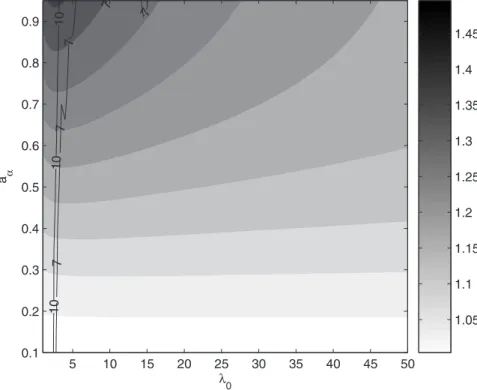
Suppose that a sample of annual maxima follows the distribution function in Eq. (8), which is described by the five parametersα0,λ0,aα,aλandδ. The Gumbel distribution
(which is characterized by two parameters, called α0(AM) and λ(AM)0 in the following) is the form that Eq. (8) would assume foraα=aλ=0, i.e. in the absence of seasonality.
20
An analysis of the error that would derive from the adoption of a Gumbel distribution in the presence of seasonal maxima is provided in the following.
HESSD
8, 4789–4811, 2011Effects of seasonality on the distributions
of hydrological extremes
P. Allamano et al.
Title Page
Abstract Introduction
Conclusions References
Tables Figures
◭ ◮
◭ ◮
Back Close
Full Screen / Esc
Printer-friendly Version
Interactive Discussion
Discussion
P
a
per
|
Dis
cussion
P
a
per
|
Discussion
P
a
per
|
Discussio
n
P
a
per
|
α0(AM)=
√ 6σAM
π ,
λ(AM)0 =exphµAM
α0 −γE i
,
(12)
where µAM is the mean and σAM the standard deviation of the samples taken from the distribution in (8) and γE is the Euler constant. We then define x
(AM)
T =
α0log[−1/λ0log[1−1/T]] as the designT-year event with the Gumbel distribution. The same event would be characterized by a return periodT∗with the seasonal distribution 5
(8). The return period ratio RT(AM) is defined by Eq. (9) as the ratio of the reference return periodT to the return periodT∗ of thexT(AM) event. In this case the relation be-tween the return period ratio and the distribution parameters cannot be expressed in closed analytical form. The ratio is computed several times by varying the parameters of Eq. (8). The values assumed byRT(AM), after considering the variation of λ0 andaα
10
and by keeping the other parameters constant, are shown in Fig. 4 (shaded areas). It can be observed thatRT(AM) assumes values up to 1.45, for high values of aα and low λ0, whereas R
(AM)
T is unaffected by the variation of the scale parameter α0 (not shown). This implies that the assumption of a Gumbel model leads to less relevant overestimation of the return period of the design event than in the POT case.
15
To check if these errors would be detectable we apply the same testing procedure as for the POT case. The application demonstrates that the test is unable, for sample dimensionsN≤50 yr, to discern between a sample generated from (8) and a Gumbel-distributed sample. In Fig. 4 the percentage of cases recognized as non-Gumbel by the Anderson-Darling test (at a 5% level) is shown by the black contour lines, for variable 20
HESSD
8, 4789–4811, 2011Effects of seasonality on the distributions
of hydrological extremes
P. Allamano et al.
Title Page
Abstract Introduction
Conclusions References
Tables Figures
◭ ◮
◭ ◮
Back Close
Full Screen / Esc
Printer-friendly Version
Interactive Discussion
Discussion
P
a
per
|
Dis
cussion
P
a
per
|
Discussion
P
a
per
|
Discussio
n
P
a
per
|
4 Case study
In this Section 294 rainfall stations located in the North-West of Italy are examined, with the aim of demonstrating the importance of precipitation seasonality in the area of study. Daily totals of precipitation depths are available between year 1913 and 1986. The peak over threshold series are extracted by imposing a threshold value of 20 mm 5
on the precipitation depths. The threshold corresponds to about λ=20 events per
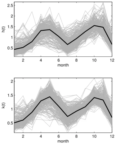
year over the whole data set, which seems a reasonable approximation for the aver-age number of significant rain events in a year. The site-specific regime curves are obtained by aggregating the exceedance amounts and the occurrence rates at the monthly timescale and by subsequently averaging the results for each station. A repre-10
sentation of the at-site regimesh(t) andk(t) (respectively, the amount and occurrence regimes divided by their mean, see Eq. (2)) is given in Fig. 5 for all the stations in the region (grey lines).
A marked seasonal behavior in both the amount and occurrence rate of the regimes emerges: in particular most of the curves are characterized by a double peak. The 15
two curves also appear to have approximately the same oscillation period and to be in phase. The time shift (δ=1÷12 months) between the two curves is determined
by varying the value of δ and evaluating, for each station, a distance measure (D) between the site-specific regimes. D is defined as the average of the absolute dif-ferences between the 12 monthly values ofh(t) andk(t). The minimumD is found in 20
correspondence ofδ=0 for 291 (out of 294) stations. The global regimes (black curves
in Fig. 5) of the mean precipitation intensity and rainfall rate, derived by averaging the station-specific curves, are then assumed to be in phase for the whole region of study. The parameters α0 and λ0 are estimated in each station as the average (over-threshold) rainfall intensity and rainfall rate. aα and aλ are estimated as functions of
25
the coefficients of variation (CV) ofα(t) andλ(t). The reasoning to find the relation
HESSD
8, 4789–4811, 2011Effects of seasonality on the distributions
of hydrological extremes
P. Allamano et al.
Title Page
Abstract Introduction
Conclusions References
Tables Figures
◭ ◮
◭ ◮
Back Close
Full Screen / Esc
Printer-friendly Version
Interactive Discussion
Discussion
P
a
per
|
Dis
cussion
P
a
per
|
Discussion
P
a
per
|
Discussio
n
P
a
per
|
Under the hypothesis of poissonianity, the cumulative distribution ofλ,FΛ(λ), can be
obtained as a derived distribution of the times of occurrence, provided that the relation
λ(t) is monotonic. To meet this condition, we restrict the domain of λ(t) to the interval [π/2n;3π/2n] (which should be multiplied by 365/2π to be expressed in days). The distribution of λ is unaffected by this assumption, due to the periodicity of the λ(t)
5
function. On this domain, the cumulative distribution of timesFT(t) is uniform, Equation (2) relatesλtot, and the cumulative distribution function ofλreads
FΛ(λ)=
1
πarcsin λ
0−λ
aλλ0
−1
2, (13)
which is valid in the domain [λ0(1−aλ);λ0(1+aλ)]. The mean and standard deviation
are respectively µλ=λ0 and σλ=aλλ0/√2 and the relation between CVλ and aλ is
10
found accordingly asaλ=√2·CVλ. Analogously, one obtainsaα=√2·CVα.
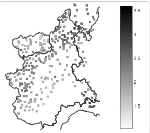
RT(POT) values are then obtained from Eq. (11) for each station, as shown in Fig. 6. Rather large values are found, pointing out the risk to significantly underestimate the design values if seasonality is neglected. When the annual maxima are considered,
RT(AM)varies between 1 and 1.45 (not shown), demonstrating that in this case the errors 15
induced by neglecting seasonality are not extremely relevant.
5 Discussion and conclusions
The effects of disregarding seasonality of extremes when evaluating the return period
of a design event are investigated. Two very simple examples are illustrated: (1) the case of using an exponential distribution to describe POT values derived from a non-20
homogeneous Poisson process (Sect. 3.1); and (2) the case of using a Gumbel distri-bution for AM values extracted from a seasonal (i.e., with time dependent parameters) distribution (Sect. 3.2). The entity of the return period overestimation (i.e., apparently less frequent extreme events) when seasonality is not accounted for is quantified by a coefficientRT. It is found that, when seasonality is ignored and threshold exceedances
HESSD
8, 4789–4811, 2011Effects of seasonality on the distributions
of hydrological extremes
P. Allamano et al.
Title Page
Abstract Introduction
Conclusions References
Tables Figures
◭ ◮
◭ ◮
Back Close
Full Screen / Esc
Printer-friendly Version
Interactive Discussion
Discussion
P
a
per
|
Dis
cussion
P
a
per
|
Discussion
P
a
per
|
Discussio
n
P
a
per
|
(POT) are analyzed, the return period of an event can be overestimated up to 7 times. Neglecting seasonality therefore corresponds to significantly underestimating the de-sign values; moreover, standard goodness-of-fit techniques are not very efficient at
recognizing the unsuitability of the non-seasonal distribution.
Resorting to peak over threshold analysis is, nevertheless, an advantageous tech-5
nique, especially in the presence of few years of observation, as acknowledged by numerous works (see e.g. Wilks, 1993; Lang et al., 1999). This allows, in fact, to capture more accurately the upper tail of the distribution, increasing at the same time the sample dimension. In this sense, the difficulties pointed out by this study in
ana-lyzing seasonal POT values should not discourage the adoption of an over-threshold 10
modelling, but rather reassert the need for accurate preliminary analyses of the data based on visual inspection of the regimes or, possibly, on unsupervised testing tech-niques (e.g., “analysis of variance” or ANOVA techtech-niques, see e.g., Salas et al., 1980; Kottegoda and Rosso, 1998).
Less relevant errors are associated to the use of the annual maximum distribution, 15
even if seasonality still induces a systematic downward bias in design value estimators. In particular, the Gumbel distribution is found to represent an acceptable choice to de-scribe the annual maxima generated by a Poisson exponential process with seasonally varying parameters. The reason behind this better performance probably lies in the greater flexibility of the Gumbel distribution (compared to the exponential).
20
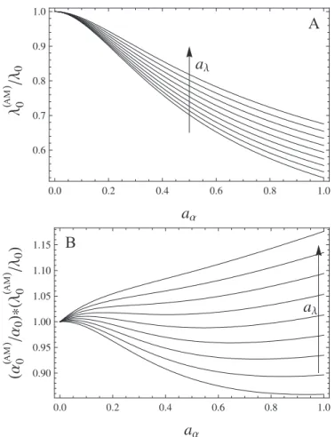
However, while the Gumbel distribution generally performs well, it is of interest to note that, in the presence of seasonality, the estimated α0(AM) and λ(AM)0 values (see Eq. (12)) lose (some of) their physical significance. In fact,α0(AM) andλ(AM)0 do not cor-respond to the average rainfall intensity and average rainfall rate,α0andλ0. In Fig. 7A the relative variations of the λ(AM)0 to λ0 ratio are shown for varying aα and aλ. It is
25
HESSD
8, 4789–4811, 2011Effects of seasonality on the distributions
of hydrological extremes
P. Allamano et al.
Title Page
Abstract Introduction
Conclusions References
Tables Figures
◭ ◮
◭ ◮
Back Close
Full Screen / Esc
Printer-friendly Version
Interactive Discussion
Discussion
P
a
per
|
Dis
cussion
P
a
per
|
Discussion
P
a
per
|
Discussio
n
P
a
per
|
parameter range. One can observe that the product values are fan-shaped around the unit value, with greater differences corresponding to higheraαvalues. This entails that
in the parameters estimation process the total amount of “over-threshold precipitation”
λ(AM)0 ·α0(AM) tends to remain constant, with lower values assumed byλbeing compen-sated by an increase in the estimated α. This systematic underestimation of λ and 5
overestimation ofα should be accounted for when the parametersλ(AM)0 andα(AM)0 are used to infer the statistical properties of the extreme-value process in the area.
In conclusion, the message we want to convey with this work is about the need of accounting for seasonality when dealing with hydro-climatic extreme values. We show that disregarding their non-homogeneity may have detrimental consequences in design 10
value estimation. Moreover, the errors may be difficult to detect by means of standard
goodness of fit testing techniques. Future work will focus on the formulation of ad-hoc metrics to identify and quantify the seasonality in hydrological extremes.
Acknowledgements. The work was funded by the Italian Ministry of Education (grants
2007HBTS85 and 2008KXN4K8).
15
References
Abramowitz, M. and Stegun, I.: Handbook of Mathematical Functions, Applied Math. Series 55, Dover Publications, 1965. 4794
Black, A. and Werritty, A.: Seasonality of flooding: a case study of North Britain, J. Hydrol., 195, 1–25, 1996. 4790
20
Buishand, T. and Demar ´e, G.: Estimation of the annual maximum distribution from samples of maxima in separate seasons, Stochastic Hydrol. Hydraul., 4, 89–103, 1990. 4791
Carter, D. and Challenor, P.: Estimating return values of environmental parameters, Quart. J. Roy. Meteor. Soc, 107, 256–266, 1981. 4791
Claps, P. and Laio, F.: Can continuous streamflow data support flood frequency analysis? An
25
HESSD
8, 4789–4811, 2011Effects of seasonality on the distributions
of hydrological extremes
P. Allamano et al.
Title Page
Abstract Introduction
Conclusions References
Tables Figures
◭ ◮
◭ ◮
Back Close
Full Screen / Esc
Printer-friendly Version
Interactive Discussion
Discussion
P
a
per
|
Dis
cussion
P
a
per
|
Discussion
P
a
per
|
Discussio
n
P
a
per
|
Coles, S.: An introduction to statistical modeling of extreme values, Springer Series in Statistics, Springer-Verlag London limited, 2001. 4794
Eagleson, P.: Climate, soil, and vegetation 1. Introduction to water balance dynamics, Water Resour. Res., 14, 705–712, 1978. 4792
Ettrick, T., Mawdlsey, J., and Metcalfe, A.: The influence of antecedent catchment conditions
5
on seasonal flood risk, Water Resour. Res., 23, 481–488, 1987. 4791
Katz, R., Parlange, M., and Naveau, P.: Statistics of extremes in hydrology, Adv. Water Resour., 25, 1287–1304, 2002. 4791
Kottegoda, N. and Rosso, R.: Statistics, probability, and reliability for civil and environmental engineers, McGraw-Hill, International Edition, 1998. 4801
10
Laio, F.: Cramer-von Mises and Anderson-Darling goodness of fit tests for extreme value distributions with unknown parameters, Water Resour. Res., 40, W09308, doi:10.1029/2004WR003204, 2004. 4796
Laio, F., Porporato, A., Ridolfi, L., and Rodriguez Iturbe, I.: Plants in water-controlles ecosys-tems: active role in hydrologic processes and response to water stress II. Probabilistic soil
15
moisture dynamics, Adv. Water Resour., 24, 707–723, 2001. 4792
Lamberti, P. and Pilati, S.: Probability distributions of annual maxima of seasonal hydrological variables, Hydrolog. Sci. J., 30, 111–135, 1985. 4791
Lang, M., Ouarda, T., and Bob ´ee, B.: Towards operational guidelines for over-threshold model-ing, J. Hydrol., 225, 103–117, 1999. 4791, 4801
20
Madsen, H., Rasmussen, P., and Rosbjerg, D.: Comparison of annual maximum series and partial duration series methods for modeling extreme hydrologic events. 1. At-site modeling, Water Resour. Res., 33, 747–757, 1997. 4791
Rasmussen, P. and Rosbjerg, D.: Risk estimation in partial duration series, Water Resour. Res., 25, 2319–2330, 1989. 4792
25
Revfeim, K.: Annual maxima and totals of seasonally varying processes, Stochastic Hydrol. Hydraul., 5, 147–153, 1991. 4791
Rodriguez Iturbe, I., Cox, D., and Isham, V.: Some models for rainfall based on stachastic point-processes, Proceedings of the Royal Society of London Series A, 410, 269–288, 1987. 4792
30
Rust, H., Maraun, D., and Osborn, T.: Modelling seasonality in extreme precipitation, Eur. Phys. J. Special Topics, 174, 2009. 4790, 4791
HESSD
8, 4789–4811, 2011Effects of seasonality on the distributions
of hydrological extremes
P. Allamano et al.
Title Page
Abstract Introduction
Conclusions References
Tables Figures
◭ ◮
◭ ◮
Back Close
Full Screen / Esc
Printer-friendly Version
Interactive Discussion
Discussion
P
a
per
|
Dis
cussion
P
a
per
|
Discussion
P
a
per
|
Discussio
n
P
a
per
|
Water Resources Publications, Littleton, Colorado, 1980. 4801
Sivapalan, M., Bl ¨oschl, G., Merz, R., and Gutknecht, D.: Linking flood frequency to long-term water balance: Incorporating effects of seasonality, Water Resour. Res., 41, W06012, doi:10.1029/2004WR003439, 2005. 4790
Todorovic, P. and Zelenhasic, E.: A stochastic model for flood analysis, Water Resour. Res., 6,
5
211–222, 1970. 4791
Viglione, A., Chirico, G., Komma, J., Woods, R., Borga, M., and Bl ¨oschl, G.: Quantifying space-time dynamics of flood event types, J. Hydrol., 394, 213–229, 2010. 4790
Villarini, G., Smith, J., Serinaldi, F., and Ntelekos, A.: Analyses of seasonal and annual maxi-mum daily discharge records for central Europe, J. Hydrol., 399, 299–312, 2011. 4790
10
HESSD
8, 4789–4811, 2011Effects of seasonality on the distributions
of hydrological extremes
P. Allamano et al.
Title Page
Abstract Introduction
Conclusions References
Tables Figures
◭ ◮
◭ ◮
Back Close
Full Screen / Esc
Printer-friendly Version
Interactive Discussion
Discussion
P
a
per
|
Dis
cussion
P
a
per
|
Discussion
P
a
per
|
Discussio
n
P
a
per
|
a
aa
lFig. 1. Example of theh(t) (solid) andk(t) (dashed) curves, see Eq. (2). The temporal shiftδ
between the seasonal peaks is indicated, as well as their amplitudes,aα andaλ. In this case
HESSD
8, 4789–4811, 2011Effects of seasonality on the distributions
of hydrological extremes
P. Allamano et al.
Title Page
Abstract Introduction
Conclusions References
Tables Figures
◭ ◮
◭ ◮
Back Close
Full Screen / Esc
Printer-friendly Version
Interactive Discussion
Discussion
P
a
per
|
Dis
cussion
P
a
per
|
Discussion
P
a
per
|
Discussio
n
P
a
per
|
Fig. 2. Sensitivity of the return periodRT(POT) to variations ofλ0andaα, withT=100 yr,δ=π,
HESSD
8, 4789–4811, 2011Effects of seasonality on the distributions
of hydrological extremes
P. Allamano et al.
Title Page
Abstract Introduction
Conclusions References
Tables Figures
◭ ◮
◭ ◮
Back Close
Full Screen / Esc
Printer-friendly Version
Interactive Discussion
Discussion
P
a
per
|
Dis
cussion
P
a
per
|
Discussion
P
a
per
|
Discussio
n
P
a
per
|
d
return period
[years]
T
(P
O
T
)
Fig. 3. Relation between the return period ratio RT(POT) and T for increasing values of δ
HESSD
8, 4789–4811, 2011Effects of seasonality on the distributions
of hydrological extremes
P. Allamano et al.
Title Page
Abstract Introduction
Conclusions References
Tables Figures
◭ ◮
◭ ◮
Back Close
Full Screen / Esc
Printer-friendly Version
Interactive Discussion
Discussion
P
a
per
|
Dis
cussion
P
a
per
|
Discussion
P
a
per
|
Discussio
n
P
a
per
|
Fig. 4.Sensitivity of the return period ratioRT(AM)to variations ofλ0andaα, withT=100 yr,n=1,
HESSD
8, 4789–4811, 2011Effects of seasonality on the distributions
of hydrological extremes
P. Allamano et al.
Title Page
Abstract Introduction
Conclusions References
Tables Figures
◭ ◮
◭ ◮
Back Close
Full Screen / Esc
Printer-friendly Version
Interactive Discussion
Discussion
P
a
per
|
Dis
cussion
P
a
per
|
Discussion
P
a
per
|
Discussio
n
P
a
per
|
2 4 6 8 10 12
0.5 1 1.5 2 2.5
month
h(t)
2 4 6 8 10 12
0.5 1 1.5 2
month
k(t)
HESSD
8, 4789–4811, 2011Effects of seasonality on the distributions
of hydrological extremes
P. Allamano et al.
Title Page
Abstract Introduction
Conclusions References
Tables Figures
◭ ◮
◭ ◮
Back Close
Full Screen / Esc
Printer-friendly Version
Interactive Discussion
Discussion
P
a
per
|
Dis
cussion
P
a
per
|
Discussion
P
a
per
|
Discussio
n
P
a
per
|
A
B
AM
AM
AM
Fig. 7. Panel A: sensitivity of theλ(AM)0 to λ0 ratio to varyingaα andaλ values (withT=100
yr,δ=0,n=1 and λ0=20 events/year). Panel B: Sensitivity of the non-dimensional product