Estimation and testing for two-dimensional diffusions in finance: exploring a semiparametric proposal

;' V

FUNDAÇÃO

GETULIO

VARGAS

ESTIMATION AND TESTING

FOR

TWO-DIMENSIONAL DIFFUSIONS IN FINANCE;

EXPLORING

A

SEMIPARAMETRIC

PROPOSAL

DISSERTAÇÃO

SUBMETIDA

À CONGREGAÇÃO

DA

ESCOLA

DE

PÓS-GRADUAÇÃO

EM

ECONOMIA

(EPGE)

PARA

OBTENÇÃO

DO

GRAU

DE

MESTRE EM ECONOMIA

POR

CRISTIAN

HUSE

RIO DE JANEIRO, RJ

Für meine Gro Peitem,

ACKNOWLEDGEMENTS

I have no words to thank Renato Flores for accepting me as a pupil in a moment

of difficulty and disbelief concerning academic life. With his help and influence, I have

chosen my professional option, besides getting conscious not of the inexistence, but of

the negligibility, of certain aspects of the career. His courses, his orientation, our

conversations and his very particular way of viewing the field of study were

fundamental to my background. Needless to say, the remainig errors that might appear

in this work should not be blamed on him, being solely mine.

I would also like to thank those teachers whose influence, if not explicitly

mentioned, is clearly reflected in the way I face life and, of course, in the following

pages. I hope this influence remains in the many I intend to write.

I would also like to thank Irina Potapenko, Mihail Lermontov and Luis

Laurencel for computational support and exchange of ideas during this work.

Financial support from CNPq/Brasil is also gratefully acknowledged.

Finally, I cannot forget to thank my family and friends for ali support. In fact, it

1.

Introduction

Derivatives are assets whose value depends on other variables. These underlying

variables can also be assets, though not necessarily, as in the case of interest rates. Futures,

forwards, swaps, caps, floors, options on stocks, or on bills, indexes, currencies, futures and

interest rates are examples of derivatives. They can be traded both in exchanges or over the

counter, and their volume is, in general, much larger than that of the underlying assets.

Fundamental landmarks in the pricing of derivatives are the Black and Scholes (1973)

and Merton (1973) papers, developed in continuous-time and using arbitrage arguments,

which pioneered a path followed by Vasicek (1977), Cox, Ingersoll and Ross (1985a, b) and

Hull and White (1987), among others. Though the pricing framework in continuous time is

generally much more tractable and elegant than the alternative discrete approximations, the

empirical literature did not follow its theoretical counterpart. Typically, the estimation of

derivative pricing models abandons the continuous time environment, restricting itself to the

data available, which are in discrete time.

Let {xt , t > 0}, the underlying process of the price of a given asset, be a diffusion

represented by the Itô stochastic differential equation

(1.1)

where

{Wt,

t > 0}

is

a standard

Brownian

motion.

The

functions

//(.)

and

o^(.)

are,

respectively, the drift (instantaneous mean) and the volatility (instantaneous variance) of the

process.

Various specifications for the drift and volatility of diffusions in finance have been

proposed. Vasicek (1977) models interest rates, r, using an Ornstein-Uhlenbeck process,

where (ju(r),o(r)) = (J3(a-r), d), a drift with the mean-reversion property and a constant

instantaneous variance. Cox, Ingersoll and Ross (1985) develop a general equilibrium model

resulting

in a process

where

(jÁf),

a{r))

= (fi(a-r),

<j rV2),

a drift

with

the

mean-reversion

property and an instantaneous variance as a linear function of the short term interest rate.

With discrete data, Lo (1988), in a pioneering paper, proposed an estimation approach

based on the method of maximum-likelihood, whose drawback is, except for very particular

cases, to require the numerical solution of a partial differential equation for each

maximum-likelihood iteration. Nelson (1990) analysed the behavior of discrete approximations when the

interval between the observations goes to zero. Duffie and Singleton (1993) and Gourieroux,

Monfort and Renault (1993) proposed the estimation of diffusions by simulation - given

parameter values, sample paths are simulated, and their moments should be as close as

possible to the sample moments. Finally, a commonly used method consists in parametrizing

the

functions

(j.(.)

and

a2(.)

and

then

discretize

the

model

before

estimating

it.

The approach proposed by Ait-Sahalia (1996) seeks to reconcile both the theoretical

and empirical literature in option pricing. Although the data are discrete, it does not resort to

discretizations of the model. Firstly, one parametrizes the drift, for instance, which guarantees

the identification of the model and makes it possible not to restrict the volatility in any way.

After imposing the parametrization, one proceeds to the following steps:

1. Estimate the drift of the diffusion, using Ordinary Least Squares (OLS);

2. Estimate nonparametrically the marginal density of the process, using kernel smoothers;

3. Given the estimated values of the drift and the marginal density function of the process,

obtain the nonparametric estimator of the volatility as a solution to the Kolmogorov

forward equation;

4. Using the volatility estimates as input, reestimate (i) the drift parameters using Feasible

Aít-Sahalia enumerates three reasons which make his approach attractive:

(i) The importance of the volatility in derivatives pricing;

(ii) The difficulty of forming an a priori idea of the functional form of the instantaneous

volatility, as it is not observed;

(iii) The availability of long time-series of daily data of spot interest rates.

The purpose of this thesis is to explore the possibilities of bivanate extensions of

Aít-Sahalia (1996)'s framework. Bivanate diffusions appear in two-factor models and are many

times treated independently. It would be interesting to have a powerful estimating method

which would allow for investigating, and testing, different relationships among the two

univariate processes.

The essay is organized as follows. Section 2 briefly recovers Ait-Sahalia's univariate

approach, while the foliowing section analyses the bivariate case. Section 4 proposes several

semiparametric estimators for the covariance between the processes. The next section applies

the bivariate approach to a pair of assets: the main stock indexes of Brazil and Argentina.

Section 6 concludes.

The main message of this thesis is that extending Aít-Sahalia (1996)'s framework to a

multivariate setting is by no means straightforward. First, the Itô's and Fokker-Planck's

frameworks do not coincide in higher dimensions, as opposed to the univariate case. As a

matter of fact, the Fokker-Planck equation turns out to be more adequate in the bivariate case

than the Itô representation. Second, even when imposing sensible assumptions on the drift and

volatility functions, one cannot obtain a direct generalization of the univariate method. In

spite of these issues, the method might be interesting as an exploratory technique for

uncovering certain relationships between the two processes, without imposing a fully

asymptotic properties of the various possible estimators, as well as to acquire a better grasp of

relevant potential applications.

2.

Univariate

Semiparametric

Estimation

of

Diffusions

Ait-Sahalia (1996) considers the univariate Kolmogorov Forward Equation (Karlin

and Taylor (1981), p. 219), or the Fokker-Planck (FP) equation, which describes the transition

densities of continuous-time Markov processes without jump:

(2.1)

f(x,t,y,n-^(ju(x)f(x,t;y,n)+^

õt õx 2 õx

where:

f(x,t;y,f) := transition density from point (y,t') to (x,t);

ju(x) := drift of the process;

cr2(x)

:= volatility

of the

process.

A first assumption concerns the drift, parametrized as in Vasicek (1977), inspired in

the Ornstein-Uhlenbeck process, which has the mean-reverting property. Parametrization of

the

drift

is fundamental

to the

identification

of

the

pair

(ju,<t2):

imposing

no

restriction

on

the

pair

makes

it impossible

to distinguish

it from

the

pair

(aju,aa2),

where

a is a constant,

when considering a discrete sample with fixed time-intervals. Supposing a general

St ôx 2 õx~

The second assumption is the stationarity of the process - or rather, that it has

converged to a steady state i.e. to a stationary distribution - which implies f{x,t;y,f) = 0

ôt

and tt(x, t) - x(x), where #() is the marginal density of the process. Multiplying both sides

of (2.2) by 7t{y) and integrating with respect to y, one obtains,

(2.3)

Using again the assumption of stationarity, it is possible to rewrite (2.3) as

(2-4)

- ' '

_2dx2

Xdl

Integrating (2.4) one obtains

(2-5)

M(x,

0Mx)

= ^

and integrating again with respect to x and using the boundary condition ;r(0) = 0

It is then possible to write the volatility as an explicit function (p(0 ;n(x)) of the marginal

density and the parameter vector characterizing the drift. If these two objects are estimated, a

semiparametric estimate of the volatility function can be obtained as:

(2.7)

Ait-Sahalia (1996) shows that the diffusion function can be identified from the

marginal density of the process at stake and from the vector parameter estimated by OLS.

Moreover, the estimator is shown to be pointwise consistent and asymptotically normal.

3.

A

Bivariate

Generalization

3.1 The Bivariate Fokker-Planck Equation

Consider now the bivariate Fokker-Planck equation, already with a parametrization on

the drift:

(3.1)

^f(xj-y^)

= -j^±(MX

where

f(x,t;y,t') := transition density from point (y,t') to (x,t);

by(x), i, j - 1,2 :- volatilities of the Fokker-Planck representation.

First, it is worth to stress the correspondence, at least locally, between the Itô

representation and the Fokker-Planck equation (Gardiner (1990), chapter 3). The bivariate

version of the Itô stochastic differential equation is:

(3.2) dxh

dx., dt

<ju(x{,x2) an(xl,x2)

(72l(Xl,X2) <T22(X,,X2)

dWu

dW. ₂₁

where x = (xj , xi), and {(Wit)i=l2, t > 0} is a standard two-dimensional Brownian motion.

The

functions

ju\(.)

and

oíí2(.),

i = 1,2

are,

respectively,

the

drift

and

the

"volatility"

of each

process, and cijj(.), i, j = 1,2, i^j are instantaneous "covariances" between the processes.

The relation between the volatilities in both representations is B = X E , where B is

the FP volatility matrix, and 2"is the Itô volatility matrix. Thus the relation between (3.1) and

(3.2), i.e. the two-dimensional case, is

(3.3) bn(x) =b2l(x) = an(x)a2l(x) + al2(x)a22(x)

To obtain an analytical solution for the bivariate version of the FP equation in the

spirit of Ait-Sahalia (1996), one needs some assumptions that make the analysis more than a

simple extension of the earlier method. First of ali, we assume stationarity of the process, and

We then introduce the following additional hypothesis: each drift depends only on its

underlying process, which means,

(3.4)

Multiplying both sides of (3.1) by the joint density jiy\ , y>2) s My), recalling that the

stationarity assumption makes the left side of (3.1) equal to zero and integratmg with respect

toy one obtains:

(3.5)

X A (//,. (x,;&)*{x))

= i 2^r(bu

(xMx))

+ -^

(bi2 (xM

Integrating now with respect to x\ and xi.

(3.6)

where ali integration constants were set to zero. In fixed-income analysis, it is quite natural to

assume ^i(O) = 7^(0) = 0. Intuitively, this means assigning a probability zero to the event

{nominal interest rate = 0}. When considering stock returns, for example, the integration

interval

considered

is [xjmin

, x"]

and

an analogous

hypothesis

is ^i(ximin)

= ^2(x2min)

= 0.

Then one obtains integration constants equal to zero once again.

If, in addition, each "variance" of the FP representation depends only on its own

(3.7)

then it is possible to write the FP "covariance" explicitly:

(3.8) bu(x) =

n(x) 1=1

i,(*,,6)

Uxyixj

-1X

A6,.(x,.)W/(x,.)

2 ,=i oxi

However, it is still necessary to identify the system (3.3), relating the FP and the Itô

volatilities.

3.2 Parametrizing Itô Volatilities

3.2.1 A General Setting

The correspondence between the FP and Itô representations, concerning their

volatilities, is much simpler in the univariate case than in the bivariate one. While the FP

equation is more convenient in operational terms when developing our estimation procedure,

the Itô representation has an intuitive appeal, especially when considering a continuous-time

counterpart of a covariance matrix. The aim of this section is to analyse (3.6) and (3.8),

according to various assumptions imposed on the perhaps most natural Itô representation

(3.2).

The most commonly used univariate volatility parametrizations in finance nowadays

are

those

of Vasicek

(1977)

and

Cox-Ingersoll-Ross

(1985),

CIR,

given

by,

respectively,

<?{x)

= c? and

o*(x)

= c?x.

These

volatilities

could

be

incorporated

into

the

model

when

passing

from the FP to the Itô representation. We must however, as said before, identify the system

(3.3). One possibility is to assume that <Ji\ = 0, what gives:

V " / 12 V / 21 V * 12 > / 22 V. f

b22

(x)

= o\2

(x)

If, for instance, (3.7) is also imposed, this would additionally imply that

cr 22(x) = cr 22{x2)

(3.10)

a?{ (x)

+ o\2

(x)

is independent

of x2.

One simple way of fulfilling this second condition (i.e. (3.10)) is to make:

(3.11) o\\(x) = o\\(xi) and an(x) = <Jl2(xi).

As it will be shown below, (3.10) and (3.11) are somewhat stringent conditions and

make the procedure more useful for a testing rather than an estimation purpose.

Another idea would be to solve system (3.9) for the cfs, obtaining:

(T2(x)

= b (x)

b*2^

= bl' ^ bl2^

~ ^ ^

b22(x) b22(x)

h (y\

(3.12) crX2{x)-.

b22 (x)

Now, again, (3.7) may be imposed but the above system shows clearly that, in

principie, both <xH (jc) and an (x) will depend on the two components of vector x.

Ali the above assumptions are not, however, sufficient to obtain an analytical solution

for either (3.6) or (3.8). As a consequence, compared to the univariate case, one needs

additional parametric assumptions. One interesting parametrization, which has also an

intuitive appeal, consists in imposing functional forms on the variances of the Itô

representation, i.e., on the diagonal terms of the instantaneous covariance matrix of the Itô

representation. In particular, consider those variances taking the functional forms of the

volatilities of the Vasicek and CIR models; this will make it possible to write explicitly the

covariance of the Itô representation as a function of the drifts and variances of both processes,

of the joint density of the process and of the marginal density of each process. We shall now

explore many forms of this specification.

3.2.2 The Double Vasicek Model

Consider the volatilities of the Itô representation. Assume, besides the identification

condition oi\ 0, that they are parametrized as constants, such as in the Vasicek model

(3.13) M*,) = Q

(722(X2) = C2

These assumptions, together with (3.10), allow us to rewrite (3.9) as

i Oi)

= <?n Oi)

+ <4 Oi)

= Ci + °n Oi

(3.14) bl2(x) = al2{xx)cr22{x2) =

Inserting (3.14) in (3.8), one obtains a nonlinear differential equation (NDE) with variable

coefficients

(3.15)

A1(T12(x1)

+ A2an(xi)a12'(xl)

+ Aicr22(xl)

+ A4

=0

where

(3.16)

(3.17)

(3.18)

(3.19)

A=c2

A2 =nx

1

3

2

(*)

dn,(xt)

ctxl

i=i dX: ,=]

In spite of the fact that the equation above shows that, once obtained the vector parameter 9,

and constants Ci and C2 it is possible to identify the covariance between the processes from

the joint density n{.,.) and the marginal densities K\{.) and ^O» by hypothesis, the solution to

(3.15) should be a function of x\ only. Nevertheless, inspection of (3.16) and (3.19) shows

that these elements are functions of the whole vector x, nothing a priori guaranteeing that the

solution, in a given case, will be independent of the X2 values. This fact makes this

specification, within the context of our proposal, more suitable for a testing procedure rather

than for estimation purposes.

3.2.3 The Double Cox-Ingersoll-Ross Model

In spite of its popularity, the Vasicek model has some undesirable features, like the

ocurrence of processes with negative interest rates. The CIR model overcomes this problem

by the convenient specification of the volatility function.

Consider once again equations (3.9). Assume, besides the identification condition cr21

= 0, that the volatilities are parametrized such as in the CIR model:

(3.20) au(xl) = Ci

a22 (x2) = C2

These assumptions, together with (3.10), allow us to rewrite (3.9) as

^11 (*1 ) = OÍl Oi ) + <?n (*1 ) = C\X

(3.21)

bn (x)

= cjn

(x, )a22

(x2)

= C2 ^au

Inserting (3.21) into (3.8), one obtains a NDE with variable coefficients formally similar to

(3.15):

(3.22) 51cr12(^1) + 52cr12(x1)íJ12'(x1) + 53cr122(x1) + 54 =0

where

(3.23) Bx=C

(3.24) 52 =*,(*,)

(3.25)

*S=I

2

(3.26)

The equations above bear the same attributes and the same problem of those from the

previous specification, so that the same comment applies.

3.3

Parametrizing

FP

Volatilities

We explore now the combination of (3.12) with (3.7). The diffusion coefficients £(.),

i=l,2, could, for instance, be specified in a "CIR fashion" as:

(3.27) bii(yi) = kiyi,i=l,2

Alternatively, one could specify them in a "Vasicek fashion" as:

(3.28) bu =£,,i = l,2

After imposing these parametrized volatilities, one may obtain a semiparametric

estimate of the FP covariance bi2(.) from (3.8). Constants h, i=l,2, must then be obtained

beforehand.

The fact that c2i = O implies that the second process will be a true CIR or Vasicek one,

so that ki may be obtained via standard methods.

A natural way to obtain an estimator of the constant in bn(.) is, first, to consider the

kernel estimator of the conditional density using its defmition:

(3-29)

4

7t

with x = (xi, x2) and y = (yi, y2), so that the numerator of the right-hand side of (3.29) is the

joint density of two observations at the time distance x = (f + At) - t' = At, which is the

interval between observations, and the denominator is the corresponding marginal density.

The (product) kernel estimators of the joint and marginal densities are given by, respectively,

and

where the kernel K{.) is a univariate function such that

(Kl)

(K2)

Jw K(u)du

= 0

(K3)ju2K(u)du=s2<<x>

and the parameter h, assumed to be the same for every kernel, is the bandwidth, or smoothing

parameter.

The marginal fx(xx \ y) of the bivariate conditional f (x \ y) will be:

(3-32)

7t(y)

By defming u = fa - X2i)/h, integrating (3.32) with respect to u, and using property (Kl) of

the kernel function, one obtains

0.33)

flMy).r

y»,>

Kh

1=1

One should now use (3.33) to compute the marginal variances for selected^ = (yij, y2j). By

defming v-(xi- xn)/h, integrating with respect to v, and using properties (Kl) and (K2) of

the kernel function, one obtains for the marginal mean:

(3.34)

and for the marginal variance

(3.35) bn = m

Fitting a Une through the points y>j = (yij, bu (yf)) plus the origin will produce an estimate for

kj.

Another idea for the estimation of k\ may be more demanding and depend on

approximations. One may recall that, for small displacements x = t - t', if the derivatives of

the FP drifts and volatilities are negligible compared of those of the transition density, the

equation to be solved is, approximately:

(3.36) f(x,t\y,f) =

-ot ,=i

subject to the initial condition

(3.37)

the solution to the FP equation will be a bivariate normal distribution whose covariance

matrix coincides with that of the FP 6's (see Gardiner (1997), section 3.5):

(3.38)

f(x,t

\y,f)

= {2n)-Nn

{dett^.í1)]}1'2

(t-t'Y

Q]T

exp^ [x-y-M(y,t';0)(t-Q]

where

B(y,t') = bn(y,t')

The equation above represents a Gaussian distribution with covariance matrix BiyJ") and

mean y + ju(y, t';9)(t-tr).

Recalling that the left hand side of (3.38) is estimable - assuming stationarity - using

(3.29)-(3.31), this opens a wide range of possibilities both for estimation and testing. With the

parametrizations at stake - in a "CIR / Vasicek fashion" - the parameter k\ is not known but, if

one estimates parameter &2 (eg. by GMM) and takes (3.8) into account, inserting it into (3.38),

b\2Íy) is eliminated and there is only one unknown in this equation - k\. One interesting

possibility is to choose a k\ which minimizes the Kullback-Leibler discrepancy measure

between the associated bivariate normal density and the one estimated nonparametncally.

Once this parameter is obtained, one gets bniy) in a straightforward manner.

If one considers the assumptions leading to (3.38) reasonable, it is even possible to test

a variety of hypotheses comparing the densities f(x, t \ y, f) resulting from the two

alternatives. For instance, one could compare a variety of parametrizations concerning both

the drifts and volatilities of the bivariate process.

4.

The

Semiparametric

Procedure

In order to implement the procedure developed in section 3.2, conceming

parametrizations on the diagonal terms of the Itô volatility matrix, we propose to replace the

drift

parameter

vector

6, the

densities

n{.,.),

m{.)

and

dnjdxi,

i=l,2,

and

the

parameters

C,,

i=l,2 by consistent estimators. The densities are estimated using kemel smoothers (see

Silverman (1986) for an introduction and Scott (1992) for an advanced treatment), while

GMM estimation after discretization of each process yields 9 and C,, i=l,2. The only

parameter to be estimated is then <j n(.), the solution of either (3.15) or (3.22) depending on

the assumptions conceming the diagonal terms of the Itô volatility matrix.

If instead one considers the implementation of the procedure suggested in section 3.3,

conceming parametrizations on the FP volatilities, we propose to estimate the drift parameter

vector 9 and the parameter &? of the FP volatility of the second process using GMM. The

densities /(. |.), /(.,.), tt(.) and fx{. |.) should be estimated using kemel smoothers. The

fírst approach suggested conceming the estimation of parameter kj could be accomphshed

using OLS estimation. The altemative, based on the density (3.38) deserves more study but,

as mentioned before, one interesting possibility could be to choose a k\ which minimizes the

Kullback-Leibler discrepancy measure between its associated normal density and the one

estimated nonparametrically. Once k\ is obtained, computation of bniy) is straightforward.

Various regularity conditions on (i) the time series dependence in the data, (ii) the

kemel actually used and (iii) the bandwidths, are needed, if asymptotic results are desired for

the estimators.

5.

An

Application

to

the Brazilian

and

Argentinian

Stock

Markets

5.1

The

Data

To illustrate our approach, we use daily (logarithmic) retums of the Ibovespa and the

Merval, which are, respectively, the main Brazilian and Argentinian stock indexes. The

sample is from October 19, 1989 to March 16, 1999, and we considered the index on market

closure. It was assumed that Fridays are followed by Mondays, with no adjustment for

weekend effects.

Although the series are clearly nonstationary in leveis (see figures 1 and 2 in Appendix

1), the returns seem to be stationary (see figures 3 and 4). An interesting feature of the returns

is the ocurrence of outliers, especially in the Brazilian series, a characteristic of emerging

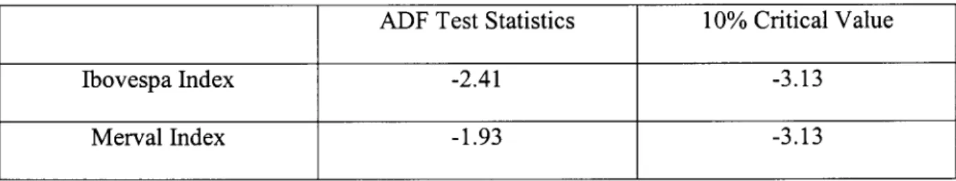
markets. The stationarity assumption was tested for both series (see Table 1), being clearly

satisfied. Table 2 shows some summary statistics for the series. One should note that the null

hypothesis of normality of the returns is clearly rejected by the Jarque-Bera test (see Davidson

and MacKinnon (1993), p. 567), mostly because of kurtosis - this feature will be mentioned

again next, when considering the density estimates. As a consequence, estimation methods

based on maximum likelihood under the normality assumption are expected to be inefficient.

TABLE 1 - Unit Root Tests

Ibovespa Index

Merval Index

ADF Test Statistics

-2.41

-1.93

10% Criticai Value

-3.13

-3.13

TABLE 2 - Basic Statistics of the Returns Mean Median Std. Dev Skewness Kurtosis

Jarque - Bera

Probability Ibovespa Retums 0.006694 0.005059 0.296752 0.273208 540.7741 Normality Test 27076466 0.000000 Merval Retums 0.001343 0.000895 0.039786 -1.750782 72.93948 459117.5 0.000000

5.2 GMM Estimation

The GMM estimates for univariate Vasicek models were obtained from the following

four moment conditions (A = 1 day) (see Karlin and Taylor (1981), p. 218, and Aít-Sahalia

(1996) for details):

(5.1)

E/t

(6)'

= E[ et+A

, rt st+A

, St+A2

- E[et+A2|

rt] , rt (et+A2

- E[st+A2|

rt])

] = 0

where

(5.2) Et+A = (rt+A - rt) - E[(rt+A - rt)| rt]

(5.3)

E[(rt+A-rt)|rt]-(l-e-pA)(a-rt)

(5.4)

22pA

One should recall that (i) this problem does not reduce to OLS, as we have an overidentified

system, (ii) these moments correspond to transitions of length A, and are not subject to

discretization bias.

The moment conditions above are just a fírst approximation to the problem. As a

matter of fact, ideally, one should also consider the off-diagonal terms of the Itô volatility

matrix, as discussed in section 3.

TABLE 3 - GMM Estimation for the Vasicek Model

a

P

a

Ibovespa Returns

3.893

x 10"J

(4.10)**

2.410

(6.51)**

7.833

x 10"J

(10.81)**

Merval Returns

1.225

x 10"J

(1.39)*

2.794

(3.87)**

3.917

x IO"2

(2.81)**

Notes: (i) The estimates reported are for daily sampling of the returns.

(ii) Heteroskedasticity-robust t statistics are in parentheses.

* Null hypotheses rejected at the 10 percent levei of significance.

** Null hypotheses rejected at the 1 percent levei of significance.

5.3 Density Estimation

The densities of both Ibovespa and Merval returns are characterized by heavy tails, as

we illustrate in this section. Consider first the joint Ibovespa and Merval returns density, in

figures 5 and 5 a in Appendix 1, and then the nonparametric marginal densities estimates for

Ibovespa and Merval returns (figures 6 and 7) compared to the normal densities with same

mean and variance of each return (figures 8 and 9). As the density estimates are inputs of the

estimation procedure, it is taking account of the heavy tails which characterize the data at

stake, although it is also worth to mention that there are several methods to handle outliers in

a more proper way, which will certainly be done in the future.

5.4

Itô

Covariance

Estimation:

The

Double

Vasicek

and

CIR

Models

Given the parameter estimates for #,, C, , i = 1,2, and the nonparametric density

estimates for n{.,.) and m(.), i=l,2, the covariance estimate ân solves (3.15) and (3.22),

respectively for the Vasicek and CIR assumptions concerning the elements of the diagonal of

the Itô covariance matrix. It must be pointed out that, somewhat improperly, we shall use in

this exercise the C, estimates obtained above. This could be avoided by considering moment

conditions which take into account the off-diagonal terms of the Itô volatility matrix, as

already mentioned in section 5.2.

However, one important question concerning the boundary conditions to be used

remains. Consider first the Vasicek model in the case of fixed income. At the point (x\jC2) =

(0,0) onemay rewrite (3.16)-(3.19) as:

(5.5) Ax = C

(5.6) A2=tt1(0)

(5.7)

4=7^

2 dx, _x,=0

(5.8)

4

2 tí

''

&,.

if we impose /ri(0) = ^(0) = ^(0,0) = 0, which is the bivariate counterpart of the boundary

condition imposed by Aít-Sahalia (1996), the result is

(5.9)

dx.

vV

*,=<>,

1/2

It is straightforward to see that one may get a complex-valued boundary condition: imposing

cr/2(0) > 0 implies that

(5.10)

dx2(x2)

dx2

dxx

x,=0

As both Ci and C2 are assumed to be strictly positive and the derivatives are likely to have

the same (positive) sign, the assumption is invalid.

Consider next the Vasicek model in the case of variable income. Assuming that

rn) =

n2(x2mm)

= 4xrn^C2mm)

= 0, one

gets,

at (x^2)

= (xi1^1),

for

(3.16)-(3.19):

(5.11)

(5.12)

(5.13)

A2 =

2 dx,

(5.14)

leading to:

(5.15)

dx. 1=1 dx..

1/2

Once again one may get a complex-valued boundary condition, what in fact happened with

the data at stake. Of course, there are several other boundary conditions to be considered but,

given the results above, several assumptions were tried, and those actually used were obtained

as follows. For the Vasicek model, assume that ximin is such that A\=Q and Aa=0, a reasonable

assumption if someone is considering the data at stake. Under such assumptions, the

differential equation (3.15), related to the Vasicek model, may then be written as

(5.16)

by straightforward calculations, one gets:

(5.17)

A2

assuming that Kj = 0, one gets:

(5.18)

Alternatively, one may assume that ai2(ximin) = ai2'(ximin) = w and that A\ = 0. This

allows us to rewrite (3.15) as:

(5.19) (A2+A3)w

The solutions are given by:

2

(5.20)

2(4

+ 4)

and

_ \l/2

(5.21)

2(4

The plots of the solution of (3.15) subject to the boundary conditions (5.18) and (5.20)

are shown in Appendix 2. An important remark is that the solutions didn't converge for a

variety of values of xy and x^.

Although each boundary condition may originate a completely different behavior of

the covariance estimate, one should notice that the shape in each of the two cases considered

does not vary too much (see figures in Appendix 2). However, fürther considerations require

the construction of a testing framework, so as to conclude whether variable x2 is an argument

of the covariance (function) estimates, a question that deserves more study in the future.

6.

Conclusions

This thesis has developed a procedure, in an exploratory levei, to estimate and test

two-dimensional diffusions, with applications to fínance. The extension of Aít-Sahalia's

univariate idea to the bivariate case is not immediate, since the solution of the corresponding

Fokker-Planck equation can easily become very difficult, if not impossible in analytical terms.

By parametrizing the drifts of both processes and imposing restnctions on the terms of the Itô

and Fokker-Planck covariance matrices, it is sometimes possible to obtain a nonparametric

estimate of the covariance between the processes. However, a delicate issue might still

remain, regarding the definition of the boundary conditions for the partial differential

equations to be actually solved.

The main message of this thesis is then that extending in a general way Aít-Sahalia

(1996)'s framework to a multivariate setting is by no means straightforward. The basic reason

is perhaps because the correspondence between the Itô and Fokker-Planck representations in

higher dimensions is not the same as in the univariate case. For the methods developed here,

the Fokker-Planck equation is more tractable than the Itô representation, suggesting that

parametrizations should be made on the latter representation. Notwithstanding, even when

imposing sensible assumptions on the drift and volatility functions, one cannot obtain a direct

generalization of the univariate method.

Some suggestions for improvement and further research include (i) the development of

the testing procedure concerning the differential equations resulting from the parametrizations

on the Itô volatilities, already mentioned in section 3.2; (ii) the investigation of the class of

diffusions whose densities may be writen in closed form, the development of a

(nonparametric) testing procedure to identify such class of diffusions, and the implementation

of the estimation and testing procedure sketched in section 3.3, including asymptotic results;

(iii) the improvement of the GMM estimation procedure presented in section 5.2; (iv) the

comparison of robust density estimation methods with the standard kernel method used in

section 5.3; (v) alternative boundary conditions for differential equations (3.15) and (3.22), as

already mentioned in section 5.4; (vi) the allowance of different bandwidths and the

abandonment of the product kernel in section 3.3, especially with the availability of more

data.

A particular case that seems to be promising is that of "causai bivariate models" in

which one of the diffusions contnbutes to the volatility of the other. The appeal of this idea is

immediate - investors could improve their hedging strategies when considering a flexible

estimator of the covariance between two (groups of) assets of a given portfolio, instead of

assuming independence among processes and estimating separately univanate diffusions.

References

Ait-Sahalia, Y. (1996): "Nonparametric Pricing of Interest Rate Derivative Securities",

Econometrica, 64, 527-560.

Black, F., and M. Scholes (1973): "The Pricing of Options and Corporate Liabilities",

Journal of Political Economy, 3, 133-155.

Cox, J., J. Ingersoll and S. Ross (1985a): "An Intertemporal General Equilibrium Model of

Asset Prices", Econometrica, 53, 363-384.

Cox, J., J. Ingersoll and S. Ross (1985b): "A Theory of the Term Structure of Interest Rates",

Econometrica, 53, 385-407.

Davidson, R., and J. G. MacKinnon (1993): "Estimation and Inference in Econometrics".

Oxford: Oxford University Press.

Duffíe, D., and K. Singleton (1993): "Simulated Moments Estimation of Markov Models of

Asset Prices", Econometrica, 61, 929-952.

Gardiner, C. W. (1997): Handbook of Stochastic Methods. New York: Springer Verlag.

Gourieroux, C, A. Monfort, and E. Renault (1993): "Indirect Inference", Journal of

Applied Econometrics, 8, S85-S118.

Hull, J. and A. White (1990): "The Pricing of Options on Assets with Stochastic Volatilities".

Journal of Finance, 42, 281-300.

Karlin, S., and H. M. Taylor (1981): A Second Course in Stochastic Processes. New York:

Academic Press.

Lo, A. W. (1988): "Maximum Likelihood Estimation of Generalized Itô Processes with

Discretely Sampled Data", Econometric Theory, 4, 231-247.

Merton, R. C. (1973): "Theory of Rational Optional Pricing", Bell Journal of Economics

and Management Science, 4, 141-183.

Nelson, D. B. (1990): "ARCH Models as Diffusion Approximations", Journal of

Econometrics, 45, 7-38.

Scott, D. W. (1992): Multivariate Density Estimation: Theoory, Practice and

Visualization. New York: Wiley.

Silverman, B. W. (1986): Density Estimation for Statistical and Data Analysis. London:

Chapman and Hall.

Vasicek, O. (1977): "An Equilibrium Characterization of the Term Structure", Journal of

Financial Economics, 5,177-188.

Appendix

1 - Figures

Ibovespa Index

500 1000

Index

Figure 1

1500 2000

Merval Index

o

o

CO

o

o

<!

O

O

CM

500 1000

Index

Figure 2

1500 2000

lbovespa Returns

CO

d

cg

d

q

d

d

500 1000 1500

Index

Figure 3

2000

Merval

Returns

d

<D O

E d

9

500 1000

Index

Figure 4

1500 2000

Joint Density: Ibovespa & Merval

r o?

3 2

''* 'O

~O

Figure 5

Joint

Density:

Ibovespa

& Merval

Figure 5a

Nonparametric Marginal Density: Ibovespa Returns

\

-0.2 -0.1 0.0 0.1

Daily Returns

Figure 6

0.2 0.3

á- 8

&

Nonparametnc Marginal Density: Merval Retums

-0.15 -0.10 -0.05 0.00

Daily Returns

Figure 7

0.05 0.10 0.15

Nonparametric Density: Ibovespa x 'Normal' Ibovespa (in circies)

\

-0.2 -0.1 0.0

Oaily Returns

Figure 6

0.1 0.2 0.3

Nonparametric Density: Merval x 'Normal' Merval (in circies)

8

2

-0.8 -0.6 -0.4 -0.2

Daily Returns

Rgure 9

0.0 0.2 0.4

Appendix

2 - Semiparametric

Covariance

Estimation

In this appendix we show the covariance estimates using the altemative boundary

conditions developed in section 5.4. First, we plot the covariance function - the solution of

(3.15) - subject to the boundary condition (5.18). Then we consider the solution of (3.15)

subject to the boundary condition (5.20).

(i)

The

Solution

of

(3.15)

Subject

to

Boundary

Condition

(5.18)

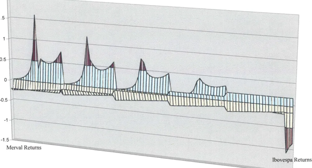
It is worth mentioning that the solution of (3.15) subject to (5.18) did not converge for

every value of xi (Ibovespa Returns). Thus, our choice was to take the values -0.2, -0.1, 0,

0.1, 0.2 for X2 (Merval Returns) to perform the numerical solution desired.

An interesting feature of the plot (Figure 10) of the solution is that it may be an

indicator of whether variable X2 is an argument of the covariance (function), although further

considerations require the construction of a testing procedure.

Figure 10 - Semiparametric Covaríance Estimate: Solution of (3.15) subject to (5.18)

-1

-1.5

Merval Returns

(ii)

The

Solution

of

(3.15)

Subject

to

Boundary

Condition

(5.20)

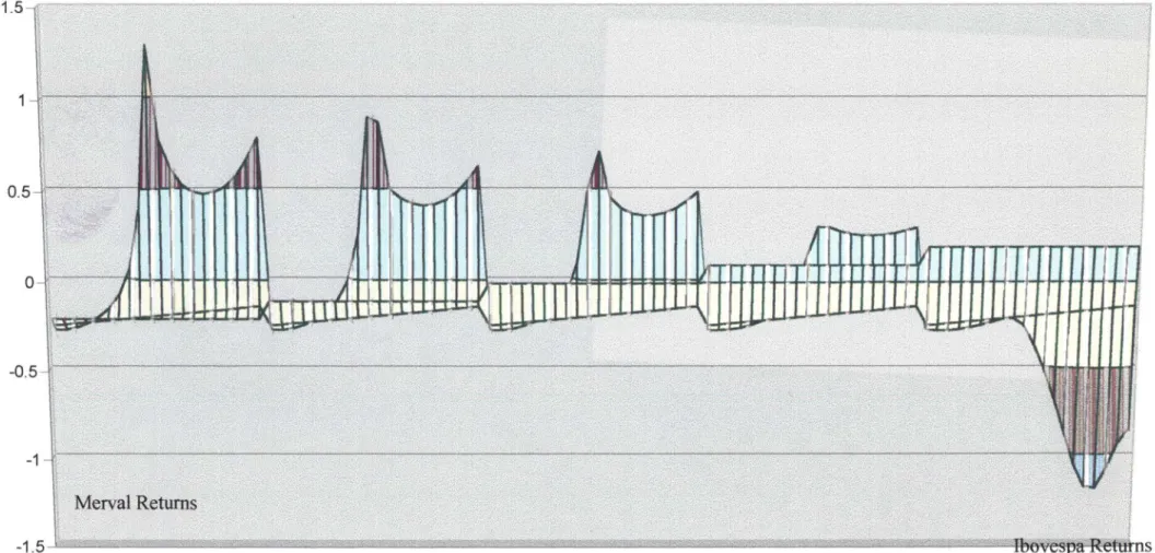
As in the previous case, the solution of (3.15) subject to (5.20) did not converge for

every value oíxj (Ibovespa Returns). Thus, our choice was to take the values -0.2, -0.1, 0, 0.1

for X2 (Merval Returns) to perform the numerical solution desired.

Just as in the previous case, the plot in Figure 11 may be an indicator of of whether

variable x2 is an argument of the covariance (function), although further considerations

require the construction of a testing procedure, a point that deserves more study in the future.

Figure 11 - Semiparametric Covariance Estimate: Solution of (3.15) subject to (5.20)

1.5--0.5

-1