Ensaios Econômicos
Escola de
Pós-Graduação
em Economia
da Fundação
Getulio Vargas
N◦ 768 ISSN 0104-8910
Life Cycle Models, Heterogeneity of Initial
Assets, and Wealth Inequality
Pedro Cavalcanti Ferreira, Diego Braz Pereira Gomes
Os artigos publicados são de inteira responsabilidade de seus autores. As
opiniões neles emitidas não exprimem, necessariamente, o ponto de vista da
Fundação Getulio Vargas.
ESCOLA DE PÓS-GRADUAÇÃO EM ECONOMIA Diretor Geral: Rubens Penha Cysne
Vice-Diretor: Aloisio Araujo
Diretor de Ensino: Carlos Eugênio da Costa Diretor de Pesquisa: Humberto Moreira
Vice-Diretores de Graduação: André Arruda Villela & Luis Henrique Bertolino Braido
Cavalcanti Ferreira, Pedro
Life Cycle Models, Heterogeneity of Initial Assets, and Wealth Inequality/ Pedro Cavalcanti Ferreira, Diego Braz Pereira Gomes – Rio de Janeiro : FGV,EPGE, 2015
37p. - (Ensaios Econômicos; 768)
Inclui bibliografia.
Life Cycle Models, Heterogeneity of Initial Assets,
and Wealth Inequality
Pedro Cavalcanti Ferreira∗ EPGE - FGV
Diego Braz Pereira Gomes ∗ EPGE - FGV
September 3, 2015
Abstract
Life cycle general equilibrium models with heterogeneous agents have a very
hard time reproducing the American wealth distribution. A common assumption
made in this literature is that all young adults enter the economy with no initial
assets. In this article, we relax this assumption – not supported by the data - and
evaluate the ability of an otherwise standard life cycle model to account for the U.S.
wealth inequality. The new feature of the model is that agents enter the economy
with assets drawn from an initial distribution of assets, which is estimated using
a non-parametric method applied to data from the Survey of Consumer Finances.
We found that heterogeneity with respect to initial wealth is key for this class of
models to replicate the data. According to our results, American inequality can be
explained almost entirely by the fact that some individuals are lucky enough to be
born into wealth, while others are born with few or no assets.
∗We would like to thank Carlos E. da Costa, Todd Schoellman, Cezar Santos, Felipe Iachan, and
1
Introduction
Wealth in the United States is highly concentrated and very unequally distributed.
Ac-cording to the Survey of Consumer Finances (SCF), in 2010, the richest 1% held one-third
of the total wealth in the economy, the richest 20% held more than 80% of total wealth,
and the Gini index of wealth was approximately 0.83.1 In addition, this inequality has
increased over time. In 1989, the richest 1% held approximately 30% of total wealth,
and the Gini index was 0.79. These facts make redistribution of wealth a central issue
in discussions of economic policy. The main tools used by economists and policymakers
to perform ex ante policy evaluations include life cycle general equilibrium models with
heterogeneous agents. It is therefore important that this class of models are able to
reproduce the main features of the American distribution of wealth.
To the best of our knowledge, no life cycle general equilibrium model with
heteroge-neous agents has been able to reproduce the American wealth distribution. In addition
toHuggett(1996), which is a standard model, other articles incorporated different
mech-anisms, such as transmission of physical and human capital (De Nardi (2004) and De
Nardi and Yang (2014)), random inheritance (Hendricks (2007a)), discount rate
het-erogeneity (Hendricks (2007b)), housing decisions and tax incentives (Cho and Francis
(2011)), idiosyncratic risk in out-of-pocket medical and nursing home expenses (Kopecky
and Koreshkova (2014)), but in one way or another, these articles fell short of the
ob-served wealth distribution.2
A common assumption made in this literature is that all young adults enter the
econ-omy with no initial assets.3 In other words, it is assumed that there is no heterogeneity
with respect to initial wealth. This assumption, however, is rejected by the data.
Ac-cording to the SCF data, the average net worth of young adults aged between 20 and
25 in 2010 was close to $24,000. The data also show that young adults are not equally
1
The measure of wealth that we consider is net worth, which includes all assets held by households (e.g., real estate, financial wealth, vehicles) net of all liabilities (e.g., mortgages and other debts). It is thus a comprehensive measure of most marketable wealth.
2
To date, the most successful economic models of U.S. wealth inequality, such as those byKrusell and Smith(1998), Quadrini(2000),Li (2002),Castañeda et al. (2003), Meh(2005), Cagetti and De Nardi
(2006),Kitao(2008), andCagetti and De Nardi(2009), do not use a realistic life cycle structure. These models use the dynastic framework or the stylized demographic structure from Gertler (1999), which was derived from theBlanchard(1985) model of perpetual youth.
3
distributed in relation to wealth. The average net worth of the 1% richest young adults
aged between 20 and 25 in 2010 was $1,433,000. This value is approximately 60 times
greater than the average of the entire age group.
In this article, we relax the assumption of no heterogeneity with respect to initial
wealth and evaluate the ability of an otherwise standard life cycle general equilibrium
model with heterogeneous agents to account for U.S. wealth inequality. In this economy,
agents differ by age, asset holdings, labor productivity, and average lifetime earnings,
and they choose their consumption, labor time and asset holdings for the next period.
Retirement is exogenous, income tax is progressive and there is uncertainty regarding the
time of death and the next period’s labor productivity. The new feature of the model is
that agents enter the economy with assets drawn from an initial distribution of assets.
After this first draw, the accumulation of assets is endogenous to the model.
This initial distribution of assets was estimated using a non-parametric method
ap-plied to the SCF data, which is an appropriate database to measure wealth inequality.
As discussed byCastañeda et al.(2003) andCagetti and De Nardi(2008), the SCF
over-samples rich households, which is especially important given the high degree of wealth
concentration observed in the data. Therefore, it provides a more accurate measure of
wealth inequality and of total wealth holdings than, for instance, the Panel Study of
Income Dynamics (PSID), which was used byHendricks(2007a) in a partial equilibrium
setting.
More importantly, the appropriate sample should not consist of only young adults.4
This is because such survey data only consider the wealth that is legally owned by the
individual, but in practice, young adults have access to their families’ wealth, which is
generally accounted for by their parents or grandparents. As evidence that young adults
have access to their families’ wealth, in 2010, 26% of household heads aged between
20 and 25 years who owned some property did not have mortgages associated with the
purchase of the primary residence.5 In the same year, 44% of young adults with some
college experience had no outstanding education loans. It is very unlikely that these
4
Hendricks(2007a) considered a sample of households with heads aged between 19 and 21. 5
young people had accumulated the resources to buy a property or to pay off student
loans in such a short period. As we will argue in the next section, there is evidence that
young adults use their family wealth.
Therefore, the wealth of young adults recorded in surveys is a lower bound of the
wealth available to them, and using that bound to estimate the initial distribution of
assets would underestimate actual wealth inequality. To prevent this, we estimated the
initial distribution of assets using data for all households and assumed that young adults
have full access to their families’ wealth when they enter the economy. We subsequently
relax this full access assumption and also consider cases where young adults access only
fractions of their families’ wealth.
We calculated the equilibrium of our model by first assuming that agents enter the
economy with zero initial assets and then assuming that agents enter with assets drawn
from the estimated distribution. As expected, our model was unable to reproduce
Amer-ican wealth inequality when all young adults enter the economy with no initial assets.
However, when we use the estimated initial distribution of assets, our model was able
to describe U.S. wealth inequality quite accurately. We reproduced the share of wealth
going to the very top households – for instance, the richest 1% has 34.8% of the total
wealth – and the wealth Gini coefficient very closely.6 Hence, according to our results,
American inequality can be explained almost entirely by the fact that some individuals
are lucky enough to be born into wealth, while others are born with few or no assets.
The remainder of the article is organized as follows. In the next section, we present
some stylized facts and discuss wealth inequality of young adults. In Section 3, we
describe our standard life cycle general equilibrium model. In Section 4, we present
the model parameterization. In Section 5, we explain the non-parametric method used
to estimate the initial distribution of assets. In Section 6, we report our findings and
quantify the role played by the initial distribution of assets in accounting for U.S. wealth
inequality. In Section 7, we perform a robustness analysis, and in Section 8, we offer
some concluding comments.
6
2
Stylized Facts
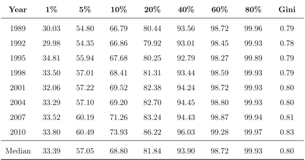
Wealth inequality has been a feature of the American economy for a long time. Table
1 presents data from the Survey of Consumer Finances of the percentage of total net
worth held by various wealth groups in different years. Although wealth concentration
has increased since 1989 – when the wealth share of the richest 5% was 6 percentage
points below that the share in 2010 – it is clear that the distribution was already very
unequal. In recent years, the net worth held by the richest 1% of households is nearly
34% of the total wealth in the economy, while the top 5% share is slightly above 60%.
The wealth Gini coefficient is above 0.80. Over the entire period, the median net worth
held by the richest 10% of households was 69% of total wealth.
There are also wide differences in the wealth distribution among young adults. The
data in Table 2 show that the average net worth of households with heads aged twenty
to twenty-five years old, according to the SCF, was twenty-four thousand dollars in 2010,
while that of one of the richest 1% (5%) of households was 1.4 million (400 thousand)
dollars in the same year. From 1989 to 2010, the wealth of a typical young man in the
richest 1% group was, on average, 61 times higher than average wealth of the age group.
Over the entire period, the median net worth held by the richest 10% of households
was 257 thousands dollars. Clearly, the distribution of wealth among young adults is
also very concentrated. Moreover, the assumption commonly made in the literature that
individuals start their working lives with zero initial assets contradicts the evidence.
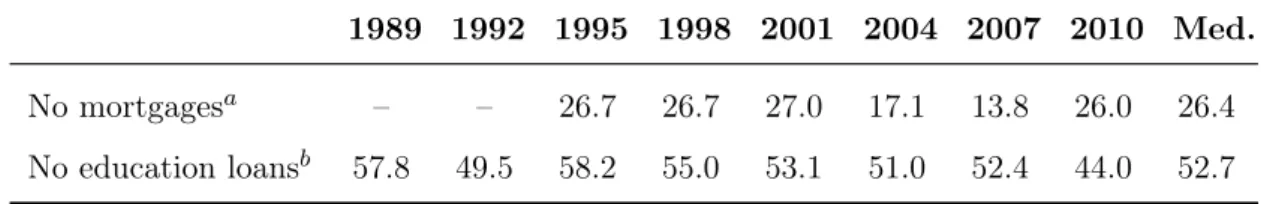
Table 3 presents additional evidence of wealth inequality among young adults. In
2010, according to the SCF, of all heads of household aged 20 to 25 who owned property,
26% had no mortgage outstanding.7 In the same year, 44% household heads in the
same age group with some college education had no education loans outstanding. Using
data from the National Postsecondary Student Aid Study (NPSAS), Kantrowitz(2014)
shows that the number of students who graduate from college without debt has been
decreasing over the last 20 years, among other reasons, because of the steep increase in
tuition, but 30% of students in 2012-13 still graduated without student loans. In addition,
according to the Pew Research Center(2014), college-educated households with student
7
Table 1: Percentage of Net Worth Held by the Richest Groups (%)
Year 1% 5% 10% 20% 40% 60% 80% Gini
1989 30.03 54.80 66.79 80.44 93.56 98.72 99.96 0.79
1992 29.98 54.35 66.86 79.92 93.01 98.45 99.93 0.78
1995 34.81 55.94 67.68 80.25 92.79 98.27 99.89 0.79
1998 33.50 57.01 68.41 81.31 93.44 98.59 99.93 0.79
2001 32.06 57.22 69.52 82.38 94.24 98.72 99.93 0.80
2004 33.29 57.10 69.20 82.70 94.45 98.80 99.93 0.80
2007 33.52 60.19 71.26 83.24 94.43 98.87 99.94 0.81
2010 33.80 60.49 73.93 86.22 96.03 99.28 99.97 0.83
Median 33.39 57.05 68.80 81.84 93.90 98.72 99.93 0.80
Source: Survey of Consumer Finances; Authors’ analysis.
Table 2: Average Net Worth Held by the Richest Groups (Aged 20-25)
Year 1% 5% 10% 20% 40% 60% 80% Avg.
1989 4,126 894 381 219 120 81 64 46
1992 815 403 250 156 90 61 46 35
1995 792 234 167 100 59 41 31 21
1998 1,436 308 198 115 63 44 33 22
2001 3,493 842 500 267 143 97 72 55
2004 1,013 418 265 155 89 60 45 33
2007 5,982 929 469 251 133 89 67 48
2010 1,433 398 217 126 69 47 35 24
Median 1,435 410 257 156 89 61 46 34
Source: Survey of Consumer Finances; Authors’ analysis. Notes: All values are in thousands of 2010 dollars.
loans to repay have lower net worth than those with no student debt ($8,700 and $64,700,
respectively).
Given the young age of these persons, and consequently, the short span of time in the
labor market, it is highly unlikely that they could finance their educations and houses
Table 3: Percentage of Young Adults Aged between 20 and 25 (%)
1989 1992 1995 1998 2001 2004 2007 2010 Med.
No mortgagesa – – 26.7 26.7 27.0 17.1 13.8 26.0 26.4
No education loansb 57.8 49.5 58.2 55.0 53.1 51.0 52.4 44.0 52.7
Source: Survey of Consumer Finances; Authors’ analysis. Notes: a Head of household aged 20–25,
owns a property but has no mortgage on the primary residence.bHead of household aged 20–25, has
some college but no education loans.
students graduated with no debt in 2007 and 2008, compared with 36% of low-income
students, and students whose parents have advanced degrees are more likely to graduate
without debt, probably because their parents have higher average incomes. More
impor-tantly, more than two-thirds of students who graduated without debt receive help paying
for tuition and fees from their parents.
In many cases, parents take out student loans themselves, the most common option
being the Parent PLUS Loan. More than 3 million Parent PLUS borrowers owe nearly
$62 billion, or approximately $20,000 per borrower, according to the Department of
Education.8 It seems clear that there is not only high wealth inequality when comparing
their own assets but also in the number of young adults who have access to their parents’
wealth (or borrowing capacity), so the numbers in the SCF database underestimate true
inequality of wealth among young people.
3
Model Economy
We built a life cycle general equilibrium model in the tradition ofİmrohoroğlu et al.(1995)
and Huggett (1996). The benchmark economy consists of a large number of heteroge-neous agents, a competitive production sector, and a government with a commitment
technology. The model is rich enough for agents to have retirement, precautionary, and
lifetime uncertainty savings motives. Time is discrete, and one model period is a year.
All shocks are independent among agents, and consequently, there is no uncertainty over
the aggregate variables, although there is uncertainty at the individual level. We describe
8
the features of the model below.
3.1 Demography
The economy is populated by agents with age j ∈ {1, . . . , J}. The population grows
exogenously at a constant rate η. Agents face exogenous uncertainty regarding the age
of death. Conditional on being alive at agej, the probability of surviving to age(j+ 1)is
given byΠj. All agents enter in the economy with agej = 1, which means thatΠ0 = 1.
Moreover, agents die with certainty at the end of ageJ, which means thatΠJ = 0. The
share of agents of age j is given byµj and can be recursively defined as
µj+1 = Πj
1 +ηµj.
3.2 Preferences
In each period of life, agents are endowed withℓunits of time, which can be split between
labor and leisure. The choice of labor time is given byl∈ L, where the set of labor times
L is finite. Agents enjoy utility from consumption, leisure, and accidental bequests, and
they maximize the discounted expected utility throughout their lives. The intertemporal
discount factor is given by β. There is a cost of working, which is treated as a loss of
leisure. The period utility function over consumption and leisure is given by
u(c, l) =
h
cγ ℓ−l−φ
1{l >0}
1−γi1−σ
1−σ ,
wherecis the consumption,γ is the share of consumption in utility,σ is the risk aversion
parameter,φis the time cost of work, and1{·}is an indicator function that maps to one
if its argument is true. The term in parentheses represents leisure time. The “warm-glow”
utility from leaving accidental bequests is given by
uB(a′) =ψ1
(ψ2+a′)γ(1−σ) 1−σ ,
whereψ1 represents the weight on the utility from bequeathing andψ2 affects its
3.3 Asset Market
Agents can acquire a one-period riskless asset in each period of their lives. We assume
that this asset provides claims to capital used in the production sector. Current asset
holdings are denoted as a ∈ A, where the set of assets A is finite. Agents enter the
economy with an endowment of assets drawn from the distribution Ω(a). The riskless
rate of return on asset holdings is denoted by r. Agents are not allowed to incur debt
at any age, so that the amount of assets carried over from age j to (j+ 1) is such that
a′≥0, wherea′ is next period’s asset holdings. For simplicity, we assume that all assets
left by the deceased are collected by the government and distributed to the live agents
as a lump-sum bequest transferB.
3.4 Labor Productivity
In each period of life, agents receive an idiosyncratic labor productivity shock that is
revealed at the beginning of the period. We denote this shock as z∈ Z, where the set
of labor productivities Z is finite. This productivity shock follows a first-order Markov
process. Conditional on having a productivity z, the probability of having next period’s
productivityz′ is given by Γ(z, z′). The invariant distribution of this Markov process is
given byΓ(z). Workers receive a wage ratewmeasured in efficiency units, which implies
that the labor income of a worker who supplieslto the labor market is given byy=wzl.
3.5 Social Security
Once agents reach the retirement age R, they automatically stop working and start
receiving a Social Security benefit. This benefit depends on the average lifetime earnings
of an agent, which is calculated by taking into account individual earnings up to age
(R−1).9 We denote the average lifetime earnings as x ∈ X, where the set of average
9
lifetime earnings X is finite. It can be recursively defined as
x′ =
x(j−1) + min y, ySS
j if j < R,
x if j≥R,
whereySS is theSocial Security Wage Base(SSWB), which is the maximum earned gross
income to which the Social Security tax applies.
Let b(x) be the Social Security benefit function, which corresponds to the Primary
Insurance Amount(PIA).10This benefit is calculated as a piecewise linear function, which
in accordance with the rules of the U.S. Social Security system, is given by
b(x) =
θ1x if x≤x1,
θ1x1+θ2(x−x1) if x1 < x≤x2,
θ1x1+θ2(x2−x1) +θ3(x−x2) if x2 < x≤ySS,
where{x1, x2}are the bend points of the function and the parameters{θ1, θ2, θ3}satisfy
0≤θ3< θ2 < θ1.
3.6 Government
Government revenues are provided from income, consumption, and Social Security taxes
and are used to finance Social Security benefits and government expenditures G. The
income tax paid by all agents is given by τY yT
, which is a progressive function of
taxable income yT. Taxable income is based on labor income and asset income and is
given byyT =y+ra. The Social Security benefit is not subject to income tax. For the
progressive income tax function, we follow the 2010 Internal Revenue Service (IRS) rules
10
and assume that
τY yT
=
τ1yT if yT ≤y1,
τ1y1+τ2 yT −y1 if y1 < yT ≤y2,
τ1y1+τ2(y2−y1) +τ3 yT −y2 if y2 < yT ≤y3,
τ1y1+ 3
X
n=2
τn(yn−yn−1) +τ4 yT −y3 if y3 < yT ≤y4,
τ1y1+ 4
X
n=2
τn(yn−yn−1) +τ5 yT −y4
if y4 < yT ≤y5,
τ1y1+ 5
X
n=2
τn(yn−yn−1) +τ6 yT −y5
if y5 < yT,
where{τ1, τ2, τ3, τ4, τ5, τ6} are the marginal income tax rates, and {y1, y2, y3, y4, y5} are
the income brackets.11 The consumption tax rate paid by all agents is given byτC, which
is proportional and levied directly on consumption. The Social Security tax rate paid
by workers is given by τSS, which is proportional and levied on the minimum of labor
income and Social Security wage base. We can formalize Social Security taxes as
TSS =τSSmin
y, ySS .
For ease of notation, we define the total taxes paid by agents, excluding the consumption
tax:
T =τY yT
+TSS.
3.7 Production Sector
We assume that there is a representative firm that acts competitively and produces a
single consumption good. This firm maximizes profits by renting capital and labor from
agents and paying an interest rate r and a wage rate w for these factors, respectively.
The production function is specified as a Cobb-Douglas function, which is given by
F(K, L) = AKαL1−α, where K and L are the aggregate capital and labor inputs, A
11
To the best of our knowledge, every article in the quantitative macroeconomic literature that con-siders a progressive income tax function uses the functional form estimated by Gouveia and Strauss
is the total factor productivity, and α is the share of capital in the output. Capital is
assumed to depreciate at a rate δ each period. We can write the problem of the firm as
max
K,L F(K, L)−(r+δ)K−wL.
3.8 Agents’ Problem
There are two groups of heterogeneous agents, workers and retirees. Workers are those
aged (R−1)and younger, while retirees are those aged R and older. Let SW and SR
be the state spaces of workers and retirees, respectively. The state vector of a worker
is given by sW = (j, z, a, x) ∈ SW, and its value function is given by VW : SW → R.
Similarly, the state vector of a retiree is given by sR = (j, a, x) ∈ SR, and its value
function is given by VR :SR → R. The agents’ problem must be solved separately for
specific age groups. Therefore, we describe the problem by dividing it between the age
groups.
For j ∈ {2, . . . , R−2}, agents are workers in the current period and will remain
workers in the next period. They choose their consumption, labor time, and the next
period’s asset holdings. Their problem can be recursively defined as
VW (sW) = max
(c,l,a′)
u(c, l) +β
ΠjEVW s′W
+ (1−Πj)uB(a′)
subject to
1 +τC
c+a′+T =y+ (1 +r)a+B,
c≥0, l∈ L, a′≥0.
Forj= 1, the only difference in relation to the above problem is in the budget constraint.
In this first period of their life, agents are “born” with initial assets drawn from an
exogenous distribution, and of course, receive no interest from the previous period’s
assets. Everything else is the same. Their budget constraint is given by
1 +τC
For j = (R−1), the only difference is in the Bellman equation. Because these agents
will be retirees in the next period, they take into account the value function of retirees
in the next period rather than the expected value function of workers.
For j ∈ {R, . . . , J −1}, agents are retirees in the current period and will remain
retirees in the next period. They choose their consumption and the next period’s asset
holdings. They no longer choose labor time because they start receiving Social Security
benefits in the current period. Their problem can be recursively defined as
VR(sR) = max
(c,a′)
u(c,0) +β
ΠjVR s′R
+ (1−Πj)uB(a′)
subject to
1 +τC
c+a′+T =b(x) + (1 +r)a+B,
c≥0, a′≥0.
Forj=J, the only difference in relation to the above problem is in the Bellman equation.
Because these agents will be dead in the next period, they no longer take into account
the value function of retirees in the next period, considering only the utility from leaving
accidental bequests.
After solving the above problems, we obtain policy functions for the control variables.
From now on, for ease of notation, we will consider s∈ S as a generic state vector in a
generic state space. Therefore, if we are considering workers, we have that s≡sW and
S ≡ SW. Similarly, if we are considering retirees, we have that s ≡ s
R and S ≡ SR.
Therefore, we can define the policy function of consumption as c :S → R+, the policy
function of labor time asl:S → L, and the policy function of next period’s asset holdings
asa′:S →R+.
3.9 Agents’ Distribution
The stationary distribution of agents among the states is described by a probability
distribution function λ :S → [0,1]. This distribution depends on the policy functions
and the exogenous stochastic processes. In this section, when used in the same equation,
the previous period. To describe how the distribution is constructed, we must divide it
among the age groups.
For j = 1, agents have just entered the economy, and there is no transition. Their
distribution depends only on the share of age groups, the initial distribution of assets,
and the invariant distribution of labor productivity, which can be defined as
λ(1, a, z) =µ1Ω(a)Γ(z).
The above expression makes explicit the main difference between our model and the rest
of the literature, which is the initial draw of an asset from a distribution.
Forj ∈ {2, . . . , R−1}, workers in the previous period remain workers in the current
period. Their distribution depends on the population growth rate, the policy function of
next period’s asset holdings, the endogenous transition of average lifetime earnings, the
survival probabilities, and the transition of labor productivities, which can be recursively
defined as
λ(s′) = 1 1 +η
X
s
1{a′(s)=a′}1{x′(s)=x′}Πj−1Γ(z, z′)λ(s).
For j = R, the only difference in relation to the above expression is that we no longer
consider the transition of labor productivities because agents become retirees at this age.
Forj ∈ {R+ 1, . . . , J}, retirees in the previous period remain retirees in the current
period. The endogenous transition of average lifetime earnings is trivial and need not
be taken into account. Their distribution depends on the population growth rate, the
policy function of next period’s asset holdings, and the survival probabilities, which can
be recursively defined as
λ(s′) = 1 1 +η
X
s
1{a′(s)=a′}Πj−1λ(s).
3.10 Equilibrium Definition
A stationary recursive competitive equilibrium for this economy consists of value
func-tions
VW, VR , policy functions{c, l, a′}, factor prices {r, w}, a consumption tax rate
τC, a lump-sum bequest transferB, and a stationary distribution of agentsλsuch that
1. The value functions
VW, VR and the policy functions {c, l, a′} solve the agents’
problem.
2. Factor prices{r, w}are determined competitively in the production sector, that is,
r=FK(K, L)−δ and w=FL(K, L).
3. The asset, labor, and consumption goods markets clear, that is,
K′ =X
s
a′(s)λ(s),
K = K
′
1 +η,
L=X
s
zl(s)λ(s),
C+K′+G=F(K, L) + (1−δ)K+E,
where the aggregate consumptionC and the aggregate initial endowment of assets
E are, respectively, given by
C =X
s
c(s)λ(s),
E=X
s j=1
aλ(s).
4. The consumption tax rateτC balances the government budget, that is,
G+X
s
b(x)λ(s) =τCC+X
s
T(s)λ(s) +X
s
(1−Πj)τY(ra′(s))
1 +η λ(s).
5. The lump-sum bequest transfer B is equal to the amount of assets left by the
deceased, that is,
B =X
s
(1−Πj)
(1 +r)a′(s)−τY(ra′(s))
4
Model Parameterization
We parameterized the model using several different data sources. Two sources of micro
data were used, the Survey of Consumer Finances (SCF)12and the Medical Expenditure
Panel Survey (MEPS).13 Our main source of macro data is the Council of Economic
Advisers(2013). Other sources of data were used and will be appropriately cited. Below we describe in detail how each parameter was estimated.
4.1 Demography
In this economy, a period corresponds to one year. We assumed that agents enter the
economy at age 20 (j = 1) and can survive to a maximum age of 100 (J = 81). We set the
population growth rateη so that the fraction of agents aged 65 and over equaled 12.55%
in equilibrium. This target was calculated using population data from Table B–34 of
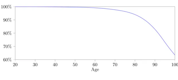
theCouncil of Economic Advisers (2013).14 The final value ofη is 2.62%. The survival
probabilities Πj were calculated using data from Table 6 of Bell and Miller(2005). We
considered the calendar year 2010 and used the average of males and females. The final
values are presented in Figure 1.
Figure 1: Survival Probabilities
20 30 40 50 60 70 80 90 100
60%
70%
80%
90%
100%
Age
12
Seehttp://www.federalreserve.gov/econresdata/scf/scfindex.htm. 13
Seehttp://meps.ahrq.gov/mepsweb/. 14
4.2 Preferences
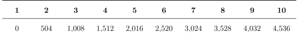
The time endowmentℓwas set to 8,760 hours, which is the total number of hours per year
(considering 365 days per year and 24 hours per day). To construct the set of labor times
L, we assumed that a worker can work from zero to 18 hours per day, but the number of
hours can only vary discreetly by multiples of two, that is, a worker can work zero, two,
four hours and so on but cannot work five or four and a half hours a day. We considered
252 working days per year, so the maximum number of hours/year is 4,536. The values of
the grid of hours are presented in Table4. We set the intertemporal discount factorβ so
that the capital-output ratio of our model equaled 3.02 in equilibrium. This target was
calculated using output data from theCouncil of Economic Advisers (2013) and capital
data from Feenstra et al.(2013).15 The final value of β in the benchmark calibration is
0.7641.
Table 4: Set of Labor Times
1 2 3 4 5 6 7 8 9 10
0 504 1,008 1,512 2,016 2,520 3,024 3,528 4,032 4,536
The share of consumption in utilityγwas set to 0.36, and the risk aversion parameter
σ was set to 3. Both values were taken from Nishiyama and Smetters (2014). We set
the time cost of work φ so that the average work hours in our model equaled 1,764
in equilibrium. This target was calculated using data from Table B–47 in Council of
Economic Advisers (2013).16 The final value of φin the benchmark calibration is 1,900
hours. The parameters of the bequest utility function were taken from French (2005).
The weight on the bequest utility ψ1 was set to 0.037 and was taken from the fourth
specification of Table 2. The curvature parameter ψ2 was set to $400,000.
15
We used the average of the ratios from 1996 to 2010. 16
4.3 Labor Productivity
We used the MEPS database to estimate the set of labor productivities Z and the
transition probabilitiesΓ(·).17 To calculate the values of the productivities we used
cross-sectional data from 1996 to 2010. For each cross-section, we considered only individuals
aged between 20 and 64 with strictly positive sample weights and strictly positive wage
incomes. All wages were converted to 2010 dollars using the annual CPI for all items.
We first calculated the weighted average of annual wages for the whole sample, which
is $43,276.31 in 2010 dollars. Next, we approximated the distribution of wages using a
histogram with bins corresponding to the 1st–25th, 26th–50th, 51st–75th, 76th–95th, and
96th–100thpercentiles.18 Within each bin, we calculated the weighted average wage using
the sample weights. Our labor productivities were then calculated as the ratios of these
averages to the average for the whole sample.
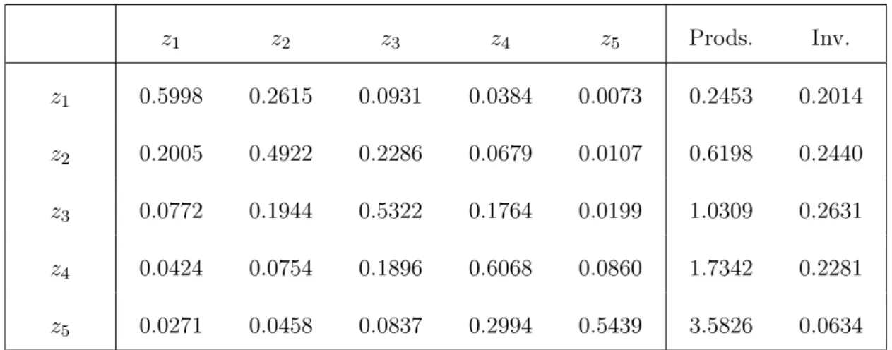
Table 5: Labor Productivities, Transition Probabilities and Invariant Distribution
z1 z2 z3 z4 z5 Prods. Inv.
z1 0.5998 0.2615 0.0931 0.0384 0.0073 0.2453 0.2014
z2 0.2005 0.4922 0.2286 0.0679 0.0107 0.6198 0.2440
z3 0.0772 0.1944 0.5322 0.1764 0.0199 1.0309 0.2631
z4 0.0424 0.0754 0.1896 0.6068 0.0860 1.7342 0.2281
z5 0.0271 0.0458 0.0837 0.2994 0.5439 3.5826 0.0634
To calculate the transition probabilities, we used a non-parametric method and data
for annual panels from 1996–1997 to 2009–2010.19 For each panel, we considered only
individuals aged between 20 and 64 with strictly positive wage incomes in both years.
17
As we want to estimate annual transitions, it is appropriate to use the MEPS database because it consists of annual panels and, therefore, no adjustment needs to be performed because of the frequency of the panel data.
18
This approximation was used to capture the long right tail of the wage distribution. 19
Constructing the transition matrix requires simply calculating the weighted fractions of
individuals who made the transition from a state z in the first year to a state z′ in the
second year.20 The values of the productivities, transition probabilities, and invariant
distribution are presented in Table5.
4.4 Social Security
The retirement ageR was set to 46, which corresponds to 65 years old in the real world.
The other parameters were collected from the official Social Security Website. The Social
Security Wage Base ySS was set to $106,800, which is the official value for 2010.21 The
bend points of the benefit function{x1, x2}were set to $9,132 and $55,032, respectively.
These are the official annualized values for 2010.22 The parameters {θ
1, θ2, θ3} were set
to their official values, which are 90%, 32%, and 15%, respectively.23 To estimate the set
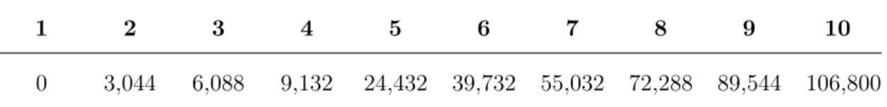
of average lifetime earnings X, we first formed a set containing the value zero, the two
bend points of the benefit function, and the Social Security Wage Base. Between each
set of points, we added two more equally spaced points to form a final set of 10 elements.
The final values are presented in Table 6.
Table 6: Set of Average Lifetime Earnings
1 2 3 4 5 6 7 8 9 10
0 3,044 6,088 9,132 24,432 39,732 55,032 72,288 89,544 106,800
4.5 Government
Government expenditures G was set to represent 18.77% of total output in
equilib-rium. This target was calculated using output and government expenditure data from
Table B–1 from the Council of Economic Advisers (2013).24 The marginal income
tax rates and income brackets were collected from the Tax Foundation (2013). The
20
The weighted fractions were calculated using the longitudinal sample weights. 21
Seehttp://www.ssa.gov/oact/cola/cbb.html. 22
Seehttp://www.ssa.gov/oact/cola/bendpoints.html. 23
Seehttp://www.ssa.gov/oact/cola/piaformula.html. 24
official values for the marginal income tax rates in 2010 were {τ1, τ2, τ3, τ4, τ5, τ6} =
{10%,15%,25%,28%,33%,35%}. For the income brackets, we took the average of the
values corresponding to single, married filing jointly or qualified widow(er), married filing
separately, and head of household filing statuses. The final values are{y1, y2, y3, y4, y5}=
{$11,362.50,$45,387.50,$101,500.00,$169,068.75,$326,943.75}. The Social Security
tax rate τSS was collected from the Social Security Administration (2014). We added
the contributions of the employee and the employer, yielding a value of 12.4%.
4.6 Production Sector
We set total factor productivityAso that output per capita in our model equaled $44,855
in equilibrium. This target was calculated using output and population data fromCouncil
of Economic Advisers (2013).25 The final value of A in the benchmark calibration is
6.07289. The share of capital in the output α was set to 0.33 and the depreciation rate
δ was set to 0.07. These values are within ranges commonly used in the literature.
5
Initial Distribution of Assets
In this section, we explain the method used to estimate the initial distribution of assets.
We used data from the SCF database and pooled all the cross-sectional data from 1989,
1992, 1995, 1998, 2001, 2004, 2007, and 2010. We considered only the records of
house-hold heads aged 20 and over. In our model, assets were identified from this database
as the net worth, and these values were converted to 2010 dollars using the annual CPI
for all items.26 The idea behind the non-parametric method is as follows. We first sort
the sample in ascending order by net worth. Then, we divided the ordered sample into
groups with the same total net worth. The support of the distribution was formed by
the average net worth of each group and the probabilities were the fraction of individuals
in each group.27
Letidenote a typical individual in the sample,nbe the size of the sample,xi be the
25
We converted the output values to 2010 dollars using the GDP implicit price deflator provided by the same source. We used the average of output per capita from 1996 to 2010.
26
In the model, assets can only take positive values, so we converted negative net worth values to zero. This is the standard procedure in the literature.
27
net worth of individuali, andwi be the sample weight associated with individuali. Note
that we need only two variables from the database, the net worth and the sample weight.
Because the first step is to sort the data in ascending order by net worth, we assume
hereafter that x1 ≤x2 ≤ · · · ≤ xn. The total net worth associated with individual i is
given byXi =wixi. This variable is a population estimate of the total net worth held by
individuals with the same characteristics as individual i. Let Si be the cumulated total
net worth up to individuali. Therefore, we have that S1 =X1 and Si =Si−1+Xi for
all i >1.
We want to divide the ordered sample into groups with the same total net worth.
However, we also want to include the zero value in the support of the distribution.
Therefore, we create a group comprising all individuals with zero net worth and m
groups that have the same total net worth, so the support of the distribution contains
(m+ 1) elements. Let j denote a typical group. We assume that j = 0 is the group in
which all individuals have zero net worth. Let Y be the constant total net worth of the
mgroups. This value is equal to the sum of total net worth of the whole sample divided
by the number of groups, that is,
Y = 1
m n X
i=1
Xi = Sn
m.
Let Ij be the interval that specifies the lower and upper limits of the cumulated
total net worth of group j. Because the sample is ordered by net worth and each group
has the same Y of total net worth, we can define these intervals as I0 = [0,0] and
Ij = ((j−1)Y, jY]for allj >0. Therefore, the estimated number of individuals in each
group is given by
Nj = n X
i=1
wi1{Si∈Ij}.
Let Aj be the average net worth of group j, with Aj =Y /Nj for allj > 0 and A0 = 0
Figure 2: Observed and Estimated Lorenz Curves
0.0 0.2 0.4 0.6 0.8 1.0
0.0 0.2 0.4 0.6 0.8 1.0 ● ● ● ● ● ● ● ● ● ● ● ● ● ● ● ● ● ● ● ● ● ● ● ● ● ● ● ● ● ● ● ● ● ● ● ● ● ● ● ● ● ● ● ● ● ● ● ● ● ● ● ● ● ● ● ● ● ● ● ● ● ● ● ● ● ● ● ● ● ● ● ● ● ● ● ● ● ● ● ● ● ● ● ● ● ● ● ● ● ● ● ● ● ● ● ● ● ● ● ● ● ● Data Estimation
are the fractions of individuals in each group and are given by
Pj = Nj m X k=0 Nk .
We used the above method to estimate a distribution with a support containing 100
elements, which means that we set m = 99. Making the connection with our model,
the set of assets A will be formed by the elements Aj and the initial distribution of
asset Ω(·) will be formed by the elements Pj. This non-parametric method has three
desirable characteristics. First, it is not necessary to make any assumptions about the
data generating process of the actual distribution. Second, as seen in Figure 2, the
estimated distribution preserves the inequality observed in the data. Third, the first
moment of the estimated distribution is equal to the first population moment. The
proposition below formally states this last result.
pop-ulation moment.
Proof. We depart from the first moment of the estimated distribution and show that it
is equal to the first population moment. For ease of notation, set
N =
m X
j=0
Nj = m X j=0 n X i=1
wi1{Si∈Ij}=
n X i=1 wi m X j=0
1{Si∈Ij} =
n X
i=1
wi.
The last equality above reflects that the intervalsIj are disjoint, which implies that each
term Si belongs to only one interval Ij. Therefore, we have that Pj = Nj/N. We can
write the first moment of the estimated distribution as
m X
j=0
PjAj = m X j=1 Nj N Y Nj = mY N = 1 N n X i=1
Xi=
1
N n X
i=1
wixi.
The last term of the above expression is exactly the first population moment. Q.E.D.
6
Results
In this section, we quantify the role played by the initial distribution of assets in
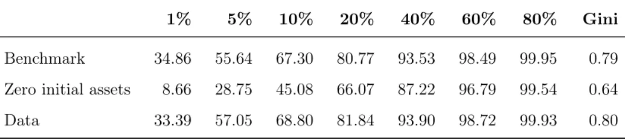
account-ing for U.S. wealth inequality. Table 7 presents our main results. Our model economy
(the “benchmark” line) describes for U.S. wealth inequality quite accurately. The Gini
indexes of the model and the data are practically the same, and the simulated share
of wealth held by the richest 1%, 5%, and 10% of the distribution is never more than
1.5 percentage points from the actual share. Compared to the results in the literature
summarized in the Appendix B, the outcome of this experiment is one of the closest to
the data. Although many studies have matched the Gini, most had difficulty replicating
the share of wealth held by the richest one or five percent. Castañeda et al. (2003), for
instance, replicates the share of the top 1% but misses the share of the top 5% by nine
percentage points.
In Table 7, for the sake of comparison and to better understand our results, we
also present the outcome of a simulation in which we calculated the equilibrium of our
model considering that all agents enter the economy with zero initial assets, the usual
assumption in the literature.28 As expected, the model considerably underestimates the
28
Table 7: Main Results
1% 5% 10% 20% 40% 60% 80% Gini
Benchmark 34.86 55.64 67.30 80.77 93.53 98.49 99.95 0.79
Zero initial assets 8.66 28.75 45.08 66.07 87.22 96.79 99.54 0.64
Data 33.39 57.05 68.80 81.84 93.90 98.72 99.93 0.80
Notes: The data values are the medians of each year according to Table1.
share of wealth held by the richest portion of the population. From the richest 1% to
the richest 10%, the absolute error of the model in relation to the data exceeds twenty
percentage points, a sizeable underestimation.
Although this last experiment cannot account for the wealth share of the richest
groups, it is important to stress that even when starting from perfect asset equality, the
model is still able to generate high inequality: the wealth Gini is 0.64, far from the perfect
zero that we started with by construction. This is because income shocks affect agents
unevenly, leading to income inequality, which in turn leads to wealth inequality. However,
these earnings shocks are not dispersed enough to allow the model reproduce observed
wealth inequality. There are not enough incentives in this case for high-income agents to
save and accumulate wealth at the same pace and in the same amounts we observe in the
data. Consequently, individuals will remain more equal, in terms of assets, throughout
the life cycle in this case.
In our benchmark simulation, we assumed that young people have access to a larger
pool of assets than those in their own names. In this sense, the initial asset distribution
has enough disparity to partially offset the low incentive to save. There is plenty evidence,
as discussed in Section2, to support this hypothesis. One assumption that, of course, is
not certain is the “correct” initial distribution or whether our strategy is close to reality.
We do know that it matches the data, but how far would we be had we assumed that
instead of full access to their family wealth, young people could only use a fraction of it?
In Table8, we repeated the main exercise assuming that young agents have access only
Table 8: Results Considering Fractions of Initial Assets
Fractions 1% 5% 10% 20% 40% Gini
0% 8.66 28.75 45.08 66.07 87.22 0.64
25% 14.23 33.75 48.68 67.63 87.12 0.66
50% 22.49 41.77 55.25 72.04 89.22 0.70
75% 29.35 49.14 61.59 76.62 91.55 0.75
100% 34.86 55.64 67.30 80.77 93.53 0.79
Data 33.39 57.05 68.80 81.84 93.90 0.80
Notes: The data values are the medians of each year according to Table1.
to a fraction of the net worth from which they draw.29
As one might expect, the smaller the fraction of assets to which young agents have
access and that they can use, the more closely we replicate the standard result in the
literature. In the limit, the 0% line, we are back to the model in which all agents start
their lives with no assets. However, for higher fractions of assets, the model is still able
to explain a large share of wealth inequality. Even when we halved the assets drawn by
each individual (the 50% line), the model explains two-thirds of the wealth share held
by the richest 1% and 73% of the richest 5%, still a close result.
The experiments in Table 8 provide an additional insight. When we multiply the
support of the initial distribution of assets by a fraction, we do not change the inequality
measures.30 This means that in each of these experiments, the concentration of the top
richest groups and the Gini index of the initial distribution are exactly the same.31
How-ever, these same measures for the aggregate distribution of the whole economy increase
with the multiplied fraction. This shows us that the inequality of the initial distribution
is not the only important factor for the model to replicate the observed inequality and
that the absolute values of the support matter. As all young adults start their working
lives poorer, the wealth distribution of the economy becomes more equal, even when the
29
We also calculated all the results in this section considering a joint initial distribution of assets and la-bor productivity. The results are practically the same, showing that our assumption of the independence of these two initial distributions is not critical.
30
Except for the 0% line, where we obtain perfect equality. 31
Figure 3: Variations in Inequality Measures
100 200 300 400
·103 10% 20% 30% 40% Initial Distribution Aggregate Distribution P ercen tage Top 1%
100 200 300 400
·103 30% 40% 50% 60% 70% Top 5%
100 200 300 400
·103 40%
50%
60%
70%
80%
Mean of Initial Asset Dist.
P
ercen
tage
Top 10%
100 200 300 400
·103 0.6
0.7 0.8 0.9
Mean of Initial Asset Dist.
Gini
inequality of the initial distribution is as high as in the data. Figure 3 illustrates this
by plotting the inequality measures of the aggregate and initial distributions of assets
as a function of the mean of the initial distribution of assets. As the mean increases,
the inequality measures of the aggregate distribution increase, while the measures of the
initial distribution remain constant.
Our life cycle model is consistent with U.S. macroeconomic data, replicating some
relevant U.S. macroeconomic variables quite closely. In Table9, we present a comparison
between some macroeconomic variables generated by the model and their corresponding
values in the data. In our benchmark simulation, we matched output per capita, average
work hours and capital per capita very closely. In the last case, the accuracy is due to
the targeting of the output per capita and capital-output ratio. The share of government
expenditures related to output was also targeted, implying very accurate government
Table 9: Observed and Estimated Macroeconomic Variables
Data* Benchmark
Output 44,855 44,855
Capital 135,454 135,313
Average work hours 1,764 1,764
Government expenditures 8,440 8,418
Social Security benefit 1,920 1,879
Interest rate 3.39% 3.94%
Hourly wage rate 17.99 18.65
*
Sources: Council of Economic Advisers(2013) andFeenstra et al. (2013). Financial values are in per capita terms. Averages from 1996 to 2010.
model was able to replicate the Social Security benefit per capita very closely, differing
from data by only 2.2% (or 41 dollars). Factor prices were also replicated without
tar-geting, with the simulated interest rate being only 0.55% higher than the data and the
hourly wage only $0.67 away from the observed hourly wage.
7
Robustness Analysis
In this section, we perform a robustness analysis to test the importance of some features
of our model in explaining U.S. wealth inequality. To do this, we performed three new
experiments. All the experiments assumed that agents enter the economy with assets
drawn from the non-parametric distribution estimated from the whole sample. However,
the parameters used to match moments of data were recalculated in each experiment.
In the first, we disregard the bequest utility uB, setting ψ
1, the weight on the utility
from bequeathing, to zero. In the second, we disregard the time cost of work, setting
the parameter φ to zero. In the third, we disregard the labor choice, forcing all agents
to work the same number of hours l. We chose the value of l so that the average hours
worked in this experiment was equal to 1,764 in equilibrium. The final value of l was
equal to 1,843.09 hours.32
These parameters and assumptions can have sizable effects on inequality. For
in-32
Table 10: Robustness Analysis
1% 5% 10% 20% 40% 60% 80% Gini
No bequest utility 35.93 57.21 67.43 79.41 92.18 97.98 99.93 0.78
No time cost of work 35.08 56.03 67.89 81.43 94.27 98.64 99.99 0.80
No labor choice 35.49 56.73 68.45 81.63 94.21 98.76 100.0 0.80
Data 33.39 57.05 68.80 81.84 93.90 98.72 99.93 0.80
Notes: The data values are the medians of each year according to Table1.
stance, we assumed that assets left by the deceased are collected by the government
and equally distributed to the surviving agents as lump-sum bequest transfers. With no
utility from bequeathing, there is less incentive to accumulate wealth, so agents save less
and consequently bequest transfers are smaller. Redistribution of wealth would decrease,
increasing inequality.
From Table10, we can see that these features alone are not critical to explaining U.S.
wealth inequality. Labor market features have only a very small impact in this case, with
no effect on the wealth Gini and only a marginal increase in the errors in the estimation
of the wealth share held by the richest groups. The impact of removing bequests from
the utility function is a bit larger, but the model still closely matches the data. It seems
that, in this economy, the initial distribution of assets has the greatest effect on wealth
inequality.
8
Conclusion
In this article, we built a standard life cycle general equilibrium model with heterogeneous
agents to explain U.S. wealth inequality. The main feature that differentiates our model
from the literature is that agents enter the economy with assets drawn from an initial
distribution of assets, so that there is heterogeneity with respect to initial wealth. We
compared the wealth distribution generated by our model with the distribution generated
by a model that assumes that all agents enter the economy with zero initial assets, an
assumption commonly adopted in the literature.
life cycle model that replicates U.S. wealth inequality. In addition, we concluded that
both inequality in the initial distribution and the absolute values of the support of the
distribution are important for the model to replicate the inequality observed in the data.
Hence, for this class of models to replicate the data, it needs to assume “enough” initial
inequality along with an appropriate initial level of wealth. Another possible mechanism,
considered in Castañeda et al. (2003), would be to assume a labor productivity process
Appendix A
Summary of Parameters
Table 11: Summary of Parameters
Parameter Value Reference
Demography
J 81 Maximum age equals 100 years old
η 2.62% Share of pop. aged 65 and over equals 12.55%
Preferences
ℓ 8,760 24 hours per day and 365 days per year
β 0.7641 Capital-output ratio equals 3.02
γ 0.36 Nishiyama and Smetters(2014)
σ 3 Nishiyama and Smetters(2014)
φ 1,900 Average work hours equals 1,764
ψ1 0.037 French(2005)
ψ2 $400,000 French(2005)
Social Security
R 46 Retirement age equals 65 years old
ySS $106,800 Official Social Security Website
x1 $9,132 Official Social Security Website
x2 $55,032 Official Social Security Website
θ1 90% Official Social Security Website
θ2 32% Official Social Security Website
θ3 15% Official Social Security Website
Government
G $8,418 Government-output ratio equals 18.77%
τ1 10% Tax Foundation(2013)
τ2 15% Tax Foundation(2013)
Table 11: Summary of Parameters
Parameter Value Reference
τ4 28% Tax Foundation(2013)
τ5 33% Tax Foundation(2013)
τ6 35% Tax Foundation(2013)
y1 $11,362.50 Tax Foundation(2013)
y2 $45,387.50 Tax Foundation(2013)
y3 $101,500.00 Tax Foundation(2013)
y4 $169,068.75 Tax Foundation(2013)
y5 $326,943.75 Tax Foundation(2013)
τSS 12.4% Social Security Administration (2014)
Production Sector
A 6.07289 Output per capita equals $44,855
α 0.33 Value commonly used in the literature
Appendix B
Results in the Literature
Table 12: Results in the Literature
Article / Data Table 1% 5% 10% 20% 40% 60% Gini
Data – 33.4 57.0 68.8 81.8 93.9 98.7 0.80
Huggett(1996) 3 11.8 35.6 – 75.5 – – 0.76
Krusell and Smith(1998) 1 24.0 55.0 73.0 88.0 – – 0.82
Quadrini(2000) XI 24.9 45.8 57.1 73.2 – – 0.74
Floden and Lindé(2001) VI 8.6 – 44.5 65.2 – – 0.65
Li(2002) 3 20.3 46.9 59.4 70.3 – – –
Nishiyama(2002) IV 19.4 41.2 55.7 74.4 93.3 99.6 0.74
Díaz et al.(2003) 10 13.7 50.6 76.6 – – – –
Castañeda et al.(2003) 7 29.9 48.1 65.0 – – – 0.79
De Nardi(2004) 5 18.0 42.0 – 79.0 95.0 100.0 0.76
Meh(2005) 8 33.6 55.2 64.7 76.6 – – 0.76
Cagetti and De Nardi(2006) 6 31.0 60.0 – 83.0 94.0 – 0.80
Hendricks(2007a) 9 11.7 35.2 51.4 71.8 91.1 98.3 0.70
Hendricks(2007b) 4 14.1 40.6 59.3 80.3 96.5 99.8 0.77
Kitao(2008) 3 35.4 58.4 66.0 80.9 96.1 99.9 0.80
Cagetti and De Nardi(2009) 3 30.0 60.0 – 85.0 95.0 – 0.82
Cho and Francis(2011) 7 – 24.3 40.8 63.4 – – 0.63
De Nardi and Yang(2014) 4 14.8 42.2 59.7 78.5 94.5 99.3 0.76
Kopecky and Koreshkova(2014) 8 18.0 51.4 70.4 – – – –
References
Bell, Felicitie C. and Michael L. Miller (2005), “Life Tables for the United States Social
Security Area 1900-2100.” Actuarial Study 120, Social Security Administration.
Blanchard, Olivier J. (1985), “Debt, Deficits, and Finite Horizons.” Journal of Political
Economy, pp. 223–247.
Cagetti, Marco and Mariacristina De Nardi (2006), “Entrepreneurship, Frictions, and
Wealth.” Journal of Political Economy, 114, pp. 835–870.
Cagetti, Marco and Mariacristina De Nardi (2008), “Wealth Inequality: Data and
Mod-els.” Macroeconomic Dynamics, 12, pp. 285–313.
Cagetti, Marco and Mariacristina De Nardi (2009), “Estate Taxation, Entrepreneurship,
and Wealth.” The American Economic Review, pp. 85–111.
Castañeda, Ana, Javier Díaz-Giménez, and José-Víctor Ríos-Rull (2003), “Accounting
for the U.S. Earnings and Wealth Inequality.” Journal of Political Economy, 111, pp. 818–857.
Cho, Sang-Wook (Stanley) and Johanna L. Francis (2011), “Tax treatment of owner
occupied housing and wealth inequality.” Journal of Macroeconomics, 33, pp. 42–60.
Council of Economic Advisers (2013), “Economic Report of the President.” Washington:
United States Government Printing Office, 2013.
De Nardi, Mariacristina (2004), “Wealth Inequality and Intergenerational Links.” The
Review of Economic Studies, 71, pp. 743–768.
De Nardi, Mariacristina and Fang Yang (2014), “Bequests and heterogeneity in retirement
wealth.” European Economic Review, 72, pp. 182–196.
Díaz, Antonia, Josep Pijoan-Mas, and José-Victor Ríos-Rull (2003), “Precautionary
Feenstra, Robert C., Robert Inklaar, and Marcel P. Timmer (2013), “The Next Genera-tion of the Penn World Table.” Database.
Floden, Martin and Jesper Lindé (2001), “Idiosyncratic Risk in the United States and
Sweden: Is There a Role for Government Insurance?” Review of Economic Dynamics, 4, pp. 406–437.
French, Eric (2005), “The Effects of Health, Wealth, and Wages on Labour Supply and
Retirement Behaviour.” The Review of Economic Studies, 72, pp. 395–427.
Gertler, Mark (1999), “Government debt and social security in a life-cycle economy.”
In Carnegie-Rochester Conference Series on Public Policy, volume 50, pp. 61–110,
Elsevier.
Gouveia, Miguel and Robert P. Strauss (1994), “Effective federal individual income tax
functions: An exploratory empirical analysis.” National Tax Journal, 47, pp. 317–39.
Guvenen, Fatih, Fatih Karahan, Serdar Ozkan, and Jae Song (2015), “What Do Data
on Millions of U.S. Workers Reveal about Life-Cycle Earnings Risk?” NBER Working Paper 20913, National Bureau of Economic Research.
Hendricks, Lutz (2007a), “Retirement Wealth and Lifetime Earnings.” International
Eco-nomic Review, 48, pp. 421–456.
Hendricks, Lutz (2007b), “How important is discount rate heterogeneity for wealth
in-equality?” Journal of Economic Dynamics and Control, 31, pp. 3042–3068.
Huggett, Mark (1996), “Wealth distribution in life-cycle economies.” Journal of Monetary
Economics, 38, pp. 469–494.
İmrohoroğlu, Ayşe, Selahattin İmrohoroğlu, and Douglas H. Joines (1995), “A life cycle
analysis of social security.” Economic Theory, 6, pp. 83–114.
Kantrowitz, Mark (2011), “Characteristics of College Students Who Graduate with No
Debt.” Student Aid Policy Analysis, FinAid.
Kantrowitz, Mark (2014), “Debt at Graduation.” Student Aid Policy Analysis, Edvisors
Kitao, Sagiri (2008), “Entrepreneurship, taxation and capital investment.” Review of Economic Dynamics, 11, pp. 44–69.
Kopecky, Karen A. and Tatyana Koreshkova (2014), “The Impact of Medical and Nursing
Home Expenses on Savings.” American Economic Journal: Macroeconomics, 6, pp. 29– 72.
Krusell, Per and Anthony A. Smith (1998), “Income and Wealth Heterogeneity in the
Macroeconomy.” Journal of Political Economy, 106, pp. 867–896.
Li, Wenli (2002), “Entrepreneurship and government subsidies: A general equilibrium
analysis.” Journal of Economic Dynamics and Control, 26, pp. 1815–1844.
Meh, Césaire A. (2005), “Entrepreneurship, wealth inequality, and taxation.” Review of
Economic Dynamics, 8, pp. 688–719.
Nishiyama, Shinichi (2002), “Bequests, Inter Vivos Transfers, and Wealth Distribution.”
Review of Economic Dynamics, 5, pp. 892–931.
Nishiyama, Shinichi and Kent Smetters (2014), “Analyzing Fiscal Policies in a
Heterogeneous-Agent Overlapping-Generations Economy.” In Handbook of Computa-tional Economics (Karl Schmedders and Kenneth L. Judd, eds.), volume 3, pp. 117– 160, Elsevier.
Pew Research Center (2014), “Young Adults, Student Debt and Economic Well-being.”
Technical report.
Quadrini, Vincenzo (2000), “Entrepreneurship, Saving, and Social Mobility.” Review of
Economic Dynamics, 3, pp. 1–40.
Social Security Administration (2014), “Update 2014.” Technical report.
Tax Foundation (2013), “U.S. Federal Individual Income Tax Rates History, 1862-2013