Artificial satellites: Resonance effects produced by terrestrial tide

(1)

ARTIFICIAL SATELLITES: RESONANCE EFFECTS PRODUCED BY

TERRESTRIAL TIDE

Jarbas Cordeiro Sampaio

UNESP- Univ. Estadual Paulista, CEP. 12516-410 Guaratinguetá-SP, Brazil, jarbascordeiro@gmail.com

Rodolpho Vilhena de Moraes

UNIFESP- Univ. Federal de São Paulo, CEP. 12231-280 São José dos Campos, SP, Brazil, rodolpho.vilhena@gmail.com

Abstract: Effects due to resonances in the orbital motion of artificial satellites disturbed by the terrestrial tide are analyzed. The nodal co-rotation resonance, apsidal co-rotation resonance and the Lidov-Kozai’s mechanism are studied. The effects of the resonances are analyzed through the variations of the metric orbital elements. Libration and circulation motions for high orbits with high eccentricities are verified for the Lidov-Kozai’s mechanism.

Keywords: Artificial Satellites. Resonances. Terrestrial Tide.

1 Introduction

Recent applications of artificial satellites require the description of the orbital motion under a precision of centime-ters. In order to attain such actual expected level, several perturbations must be considered simultaneously, as well as resonant effects. Also for the analysis of the coupled effects it is mandatory the knowledge of each effect take separately.

The resonant dynamics involving the orbital motion of artificial satellites have been extensively used for commu-nication and navigation, for example, justifying the study of resonant orbits in the last years (Rossi 2008, Formiga and Vilhena de Moraes 2008, Sampaio et. al. 2011). This studies are done using orbital perturbations such as due to the geopotential, lunisolar perturbations, solar radiation pressure, spin-orbit coupling, considering commensurabil-ities between the artificial satellite’s mean motion and the Earth’s rotational motion. The perturbation considered in this work is the terrestrial tide.

The influence of resonances in the orbital motion problem perturbed by tides has been observed by Kaula (1969), Kozai (1965), Sampaio and Vilhena de Moraes (2008) and Sampaio (2009).

In this work the objective is to analyze the nodal co-rotation resonance , apsidal co-rotation resonance and the Lidov-Kozai’s mechanism related to this problem.

2 The terrestrial tide effect 2.1 The disturbing function

The disturbing function due to the tide effect can be written as (Kozai 1973, Kozai 1965):

ROE =n21β

R5

r3

_a

1

r1

3

k2P2(cos(θ)) (1)

wherek2 is the Love’s number;β is the reduced massm1/(m+m1);n1is given byG(m+m1)/a31, G is the

gravitational constant, m is the mass of the Earth,m1 is the mass of the Moon anda1 is the semi-major axis

of the Moon around the Earth; r is the geocentric distance of the satellite; r1 is the geocentric distance of the

Moon;P2(cos(θ))is the second order Legendre polynomial in the development of the potential that describes the

(2)

ROC =ROCS(a, a1, e, I, I1) +ROCLP(a, a1, e, I, I1, ω,Ω,Ω1) (2)

and then, the secular part can be put in the following form:

ROCS = 1 32a3n1

2

β R5k2(2 + 27e 2

(cos (I))2(cos (I1)) 2

+18 (cos (I))2(cos (I1)) 2

−9e2

(cos (I1)) 2

−9e2(cos (I))2−6 (cos (I1)) 2

+ 3e2−6 (cos (I))2) (3)

The long period terms are given by:

ROCLP =− 3 128a3n1

2

β R5k2(−6e 2

(cos (I))2cos (2ω) + 6e2cos (2ω)

−12e2sin (I) sin (I1) cos (I1) cos (2ω−Ω + Ω1)

+12e2

sin (I) sin (I1) cos (I1) cos (−2ω−Ω + Ω1)

−48e2

sin (I) sin (I1) cos (I) cos (I1) cos (−Ω + Ω1)

+12e2(cos (I))2cos (2 Ω1−2 Ω)

+3e2

(cos (I1)) 2

cos (2 Ω1−2 Ω + 2ω)

+3e2

(cos (I1)) 2

cos (2 Ω1−2 Ω−2ω)

−6e2

cos (I) cos (2 Ω1−2 Ω−2ω)

−8 (cos (I))2(cos (I1)) 2

cos (2 Ω1−2 Ω)

−12e2(cos (I))2(cos (I1)) 2

cos (2 Ω1−2 Ω)

+3e2

(cos (I))2(cos (I1)) 2

cos (2 Ω1−2 Ω−2ω)

−6e2

cos (I) (cos (I1)) 2

cos (2 Ω1−2 Ω + 2ω)

+3e2

(cos (I))2(cos (I1)) 2

cos (2 Ω1−2 Ω + 2ω)

−18e2

(cos (I1)) 2

cos (2ω)

+18e2(cos (I))2(cos (I1)) 2

cos (2ω)

−8 cos (2 Ω1−2 Ω)

+12e2

sin (I) sin (I1) cos (I) cos (I1) cos (−2ω−Ω + Ω1)

+6e2

cos (I) (cos (I1)) 2

cos (2 Ω1−2 Ω−2ω)

−32 sin (I) sin (I1) cos (I) cos (I1) cos (−Ω + Ω1)

+8 (cos (I1)) 2

cos (2 Ω1−2 Ω)

+12e2

sin (I) sin (I1) cos (I) cos (I1) cos (2ω−Ω + Ω1)

+12e2(cos (I1)) 2

cos (2 Ω1−2 Ω)−3e 2

(cos (i))2cos (2 Ω1−2 Ω + 2ω)

−3e2

(cos (I))2cos (2 Ω1−2 Ω−2ω) + 6e2cos (I) cos (2 Ω1−2 Ω + 2ω)

−3e2

cos (2 Ω1−2 Ω + 2ω)−12e2cos (2 Ω1−2 Ω)

−3e2

cos (2 Ω1−2 Ω−2ω) + 8 (cos (I)) 2

cos (2 Ω1−2 Ω)) (4)

3 The nodal co-rotation resonance

Initially, the analysis of the resonance will be done through the nodal co-rotation resonance, due to the argument (Ω-Ω1) in the long period part of the disturbing function. Considering thatΩ = Ω0+nΩt, will be considered here

(3)

3.1 Terrestrial tide

Through the Lagrange planetary equations the following result for the precession of the ascen-ding node longitude

Ωcan be obtained:

nΩ=−

3 16

n12β R5k2cos (I)

na5√₁

−e2 (9e 2

(cos (I1)) 2

+ 6 (cos (I1)) 2

−3e2

−2) (5)

with

n2

=Gm

a3 (6)

The family of orbits with nodal co-rotation resonance can be obtained isolating the semi-major axis (a) and using the Eqs. (5) and (6) we get:

a= 7 s

9 256

1

GmnΩ2(1−e2)

(n1 2

β2R10k2 2

cos(I)2(9e2cos(I1) 2

+6cos(I1) 2

−3e2

−2)2

)1/7

(7)

Due to the nodal co-rotation condition we get:

nΩ=nΩ1 (8)

where the period ofnΩ1 is about 18.6 years (Roncoli 2005). We also have:

nΩ1 = 2π

T (9)

being T the period of 18.6 years.

Therefore, it was derived an equation for the semi-major axis of the satellite as a function of the eccentricity and inclination . The other terms that appear in the Eq. (7) are constants.

(4)

I=10 degrees I=20 degrees I=30 degrees I=40 degrees I=50 degrees I=60 degrees I=70 degrees I=80 degrees

e

0.1 0.2 0.3 0.4 0.5 0.6 0.7 0.8 0.9 a (m)

600,000 700,000 800,000 900,000 1,000,000 1,100,000 1,200,000 1,300,000 1,400,000 1,500,000

Figure 1. Semi-major axis a function of the eccentricity for some inclination values (Nodal co-rotation resonance)

The analysis of this type of resonance is not viable for the exact 1:1 resonance, since, in this case we will get semi-major axis smaller than the Earth’s radius. But it can be studied what happens whennΩapproaches to zero

in the region next to the 1:1 resonance. It can be observed that whennΩdecreases about two orders of magnitude,

possible values for the semi-major axis begin to appear considering high eccentricities. Figure 2 shows a simulation consideringnΩnear to zero.

e

0.1 0.2 0.3 0.4 0.5 0.6 0.7 0.8 0.9 a (m)

3,000,000 4,000,000 5,000,000 6,000,000 7,000,000

Figure 2. Variation of the semi-major axis with the eccentricity for some inclinations (nodal co-rotational resonance forn_Ωnear to zero)

It is interesting to question how the occurrence of a quasi-commensurability can affect the motion of an artificial satellite. Of course, the more next to an entire number is the ratio between the periods, but the artificial satellite can be affected with this effect (Callegari Jr 2006). This can be observed in Fig. 2.

4 The apsidal co-rotation resonance

Another analysis that is also done in this work is about the argument (2ω−Ω + Ω1) present in the disturbing

function due to the terrestrial tide. In this case, the exact resonance between the argument of perigee and the longitude of the ascending node of the disturbing body is 2:1.

(5)

nω=

3 16na5√₁

−e2n1 2

β R5

k2(15 (cos (I)) 2

(cos (I1)) 2

−3 (cos (I1)) 2

+3e2

(cos (I1)) 2

−5 (cos (I))2+ 1−e2

) (10)

Inserting in the Eq. (10) the mean motion of the satellite given by Eq. (6) and isolating the value of the semi-major axis (a) we get:

a= 7 s

9 256

n14β2R10k22

Gmn2

ω(1−e2)

((15cos2(I)cos2(I1)−3cos 2

(I1)

+3e2cos2(I1)−5cos 2

(I) + 1−e2)2)1/7 (11)

Figure 3 shows the variation ofawith respect the eccentricity(0.0001≤e≤0.9), considering some values for the inclination.

e

0.1 0.2 0.3 0.4 0.5 0.6 0.7 0.8 0.9 a (m)

200,000 400,000 600,000 800,000 1,000,000 1,200,000

Figure 3. Apsidal co-rotation resonance: Variation of the semi-major axis with respect the eccentricity

In the Fig. (3), a great variation in the semi-major axis can be observed for some given inclinations and eccen-tricities. A simulation shows that for small variations of inclination, above600_{, and for high eccentricities, large}

variations occur in the semi-major axis. This phenomenon motivated the study of the Lidov-Koza’s mechanism that will be seen in the next section.

5 Lidov-Kozai’s mechanism

In this section an analysis of resonance, involving the argument2ω, is done through the distur-bing function. This kind of phenomenon was first observed by Kozai (1962) and Lidov (1962) and is known as the Lidov-Kozai’s mechanism. The Lidov-Lidov-Kozai’s mechanism has been studied for asteroids as in Kozai (1962), for Uranus’s satellites as Kinoshita and Nakai (1999, 2007), for Jupiter’s satellites as in Yokoyama et. al. (2003) and for artificial satellite orbiting the Moon as in Carvalho et. al. (2008).

(6)

ULK = 1 32a3n1

2

β R5

k2(2 + 27e2(cos (I)) 2

(cos (I1)) 2

+ 18 (cos (I1)) 2

(cos (I))2

−9e2(cos (I1)) 2

−9e2(cos (I))2−6 (cos (I1)) 2

+ 3e2−6 (cos (I))2)

+ 3

128a3n1 2

β R5k2(6e 2

(cos (I))2cos (2ω)−6e2cos (2ω) +18e2

(cos (I1)) 2

cos (2ω)−18e2

(cos (I))2(cos (I1)) 2

cos (2ω)) (12)

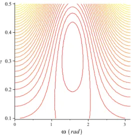
As it was done by Kinoshita and Nakai (1999, 2007), graphics for curves of the same energy in the (ω,e) plane will be done here. The study of the Lidov-Kozai’s mechanism is based on the parameter h, related with the z component of the angular momentum, given by:

h= (1−e2

)cos2

(I) =const. (13)

To generate the energy’s curves, firstly the Eq. (12) must be written in terms of the eccentricity, of the argument of perigee and of the parameter h.

This can be done using Eq. (13).

As an example, it will be initially considered here a semi-major axis of about 6960 Km for the orbit of the artificial satellite.

Figures (4) to (8) present the (ω, e) plane for some values of h.

w rad

0 1 2 3

e

0.1 0.2 0.3 0.4 0.5 0.6 0.7 0.8

(7)

w rad

0 1 2 3

e

0.1 0.2 0.3 0.4 0.5

Figure 5. (ω, e) plane for h=0.3

w rad

0 1 2 3

e

0.2 0.3 0.4 0.5 0.6

w rad

0 1 2 3

e

0.2 0.3 0.4 0.5 0.6 0.7

(8)

w rad

0 1 2 3

e

0.3 0.4 0.5 0.6 0.7

For the considered semi-major axis we found a libration motion for small values of h ( h=0.1 and h=0.3) and circulation for values near to 1 (h=0.7 and h=0.9). However, the libration and circulation motions shown in Figs. (4) to (8) occur for high eccentricities, which would be a not practical orbit. In fact, with the adopted semi-major axis, this would result perigee distance shorter than the Earth’s radius.

For an artificial satellite orbiting the Earth, the Lidov-Kozai’s mechanism would have influence, through the tide perturbation, for orbital semi-major axis greater than the one presented previously.

Analyzing the orbit of a satellite with semi-major axis of about 26500km, it is observed that as the eccentricity is greater than 0.75, the distance of perigee is near to the terrestrial surface and can be affected significantly by other disturbing forces such as atmospheric drag, or even collide with the Earth’s surface if the eccentricity reach 0.8. Starting from (e=0.75), when the eccentricity decreases, the perigee distance of the satellite became not as near from the terrestrial surface as in the precedent case.

Figures (9) to (17) show the (ω, e) plane for h varying from 0.1 to 0.9.

w rad

0 1 2 3

e

0.1 0.2 0.3 0.4 0.5 0.6 0.7 0.8

(9)

w rad

0 1 2 3

e

0.2 0.3 0.4 0.5 0.6 0.7 0.8

w rad

0 1 2 3

e

0.1 0.2 0.3 0.4 0.5

w rad

0 1 2 3

e

0.2 0.3 0.4 0.5

(10)

w rad

0 1 2 3

e

0.3 0.4 0.5 0.6 0.7 0.8

w rad

0 1 2 3

e

0.3 0.4 0.5 0.6 0.7 0.8

w rad

0 1 2 3

e

0.3 0.4 0.5 0.6 0.7 0.8

(11)

w rad

0 1 2 3

e

0.3 0.4 0.5 0.6 0.7 0.8

w rad

0 1 2 3

e

0.3 0.4 0.5 0.6 0.7 0.8

Figure 17. (ω, e) plane for h=0.9

For a satellite with the considered semi-major axis, and with the considered ranges for the variation of the constant h, a libration motion is possible when0.1≤h≤0.3. This can be observed in the Figs. (9) to (17). For values of h near to 0.1 librations occur but due to the high eccentricities, collision can occur with the Earth.

6 Conclusion

Some influences of the terrestrial tide on the orbital motion of artificial satellites were analyzed and the existence of resonances that can affect the motion was studied. Three types of resonance were analyzed: the nodal co-rotation resonance, the apsidal resonance and the Kozai’s resonance.

According to Kozai (1965), the most important resonant term expected in the present study is the term with ar-gumentΩ−Ω1in the Lagrange equation providing time variation for the inclination. The Lagrange equations

for the time variation of the eccentricity and for the longitude of the ascending node, also present terms with this argument.

Beyond the nodal co-rotation resonance, was also analyzed the influence on the orbital motion of the apsidal co-rotation resonance, relating the argument of pericentre and the longitude of the ascending node of the Moon, through a resonance of the type 2:1.

(12)

axis of about 26500 km, where the tidal effects in the orbital elements are still appreciable, there are possibilities of libration for h=0.2 and h=0.3 and circulation for values greater than h=0.3. For h=0.2, considering the range of values of eccentricity varying from 0.1 to 0.7, the inclination varies with values ranging from63.290

to51.230

for the prograde motion and116.710

to128.770

for the retrograde motion. For h=0.3 the eccentricity varies from 0.1 to 0.5. This corresponds to a variation of the inclination of56.600

to50.770

for the prograde motion and for the retrograde motion of123.400

to129.230

.

7 Acknowledgments

This work was accomplished with support of the CAPES, FAPESP under the contract No2009/00735-5 and 2006/04997-6, SP-Brazil, and CNPQ (Process: 300952 / 2008-2).

8 References

Callegari Jr., N., Ressonâncias e marés em sistemas de satélites naturais. Revista Latino-Americana de Educação em Astronomia - RELEA, 3, pp. 39-57, 2006.

Carvalho, J. P. dos S.; Vilhena de Moraes, R. and Prado, A. F. B. A., Perturbações orbitais: não esfericidade da lua e terceiro corpo. In: XIV Colóquio brasileiro de dinâmica orbital, Águas de Lindóia-SP, 2008.

Formiga, J. K. S. and Vilhena de Moraes, R., Orbital Characteristics of Artificial Satellites in Resonance and the Correspondent Geopotencial Coefficients. Journal of Aerospace Engineering, Sciences and Applications, May-Aug. 2008, Vol. I, No 2.

Kaula, W. M., Tidal Friction with Latitude-Dependent Amplitude and Phase Angle. The Astronomical Journal, Vol. 74, no9, 1969.

Kinoshita, H. and Nakai, H. Analytical Solution of the Kozai Resonance and its Application. Celestial Mech Dyn Astr 75, pp. 125-147, 1999.

Kinoshita, H. and Nakai, H., General solution of the mechanism. Celestial Mech Dyn Astr 98, pp. 67-74, 2007. Kozai, Y, A new method to compute lunisolar perturbations in satellite motions. Massachusetts: Smithsonian Inst.

Astrophysical Observatory, Cambridge, 1973.

Kozai, Y. Effects of the Tidal Deformation of the Earth on the Motion of Close Earth Satellites. Mitaka: Tokyo Astronomical Observatory. July, 23, 1965.

Kozai, Y., Secular Perturbations of Asteroids with High Inclination and Eccentricity. Massachusetts, The Astro-nomical Journal vol. 67, no9, 1962.

Lidov, M. L., The evolution of orbits of artificial satellites of planets under the action of gravitational perturbation of external bodies. Planet. Space Sci. 9, pp. 719-759, 1962.

Roncoli, R. B., Lunar Constants and Models Document. JPL: Jet Propulsion Laboratory. California, 2005. Rossi, A., Resonant dynamics of Medium Earth Orbits: space debris issues. Celestial Mechanics and Dynamical

Astronomy, 100, pp. 267-286, 2008.

Sampaio, J. C., Vilhena de Moraes, R. and Fernandes, S. S., Artificial Satellites Dynamics: Resonant Effects. 22nd International Symposium on Space Flight Dynamics, São José dos Campos, 2011.

Sampaio, J. C., Efeitos de maré no movimento orbital de satélites artificiais. 2009, 164f. Dissertação de Mestrado - Faculdade de Engenharia do Campus de Guaratinguetá, Universidade Estadual Paulista, Guaratinguetá. Sampaio, J. C. and Vilhena de Moraes, R., O Efeito de Maré Terrestre e suas Implicações para Órbitas de Satélites

Artificiais. XIV CBDO, 2008.