Motion of a falling drop with accretion using Newtonian methods.

Motion of a falling drop with accretion using Newtonian methods

G. Hernandez

, G. del Valle

, I. Campos

y J.L. Jimenez

1_{Area de F´ısica At´omica y Molecular Aplicada, Divisi´on de Ciencias B´asicas e Ingenier´ıa,}

Universidad Aut´onoma Metropolitana, Azcapotzalco, D.F., M´exico

1_{Departamento de F´ısica, Facultad de Ciencias, Universidad Nacional Aut´onoma de M´exico, D.F., M´exico} 1_{Departamento de F´ısica, Divisi´on de Ciencias B´asicas e Ingenier´ıa,}

Universidad Aut´onoma Metropolitana, Iztapalapa, D.F., M´exico

Recebido em 10/9/2010; Aceito em 24/6/2011; Publicado em 10/10/2011

The motion of a falling drop whose mass grows by accretion is studied with Newtonian methods to the point of finding the position as a function of time. The equation of motion applied is the equation of motion of continuum mechanics in its Eulerian or space formulation. We study three examples of laws of accretion: mass growing linearly with time, mass growing linearly with the surface of the drop and mass growing proportionally to the product of surface and velocity. These examples are sometimes left as exercises, without further discussion, asking only forv(z), or the final velocity. We also show that the solutions have the correct limit of a particle of

constant mass in free fall and of such a particle with friction linear in the velocity.

Keywords: variable mass systems, accretion.

Se estudia, mediante m´etodos Newtonianos, el movimiento de una gota que cae y cuya masa crece por acreci´on; se encuentra detalladamente la posici´on como funci´on del tiempo. La ecuaci´on de movimiento aplicada es la ecuaci´on de movimiento de la mec´anica de medios cont´ınuos en su forma Euleriana o espacial. Estudiamos tres ejemplos de leyes de acreci´on: masa increment´andose linealmente con el tiempo, masa increment´andose propocionalmente a la superficie de la gota e incremento de la masa proporcional al producto de la superficie por la velocidad. Tambi´en mostramos que las soluciones tienen el l´ımite correcto, el de una part´ıcula, con masa constante, en ca´ıda libre y el de esa part´ıcula con fricci´on lineal en la velocidad.

Palabras-clave:sistemas de masa variable, acreci´on.

1. Introduction

The motion of systems with variable mass has concep-tual and mathematical difficulties that make its treat-ment a challenge for teachers and students alike. The typical example is the rocket, discussed in many texts without beginning from an equation of motion, and rather applying conservation of momentum in a clever way. Other examples are the motion of a rope falling from a table, a conveyor on which sand is dropped, and a raindrop whose mass grows by accretion. In this work we solve in detail this last problem by Newtonian methods considering three specific laws of accretion. The relevance of this problem in several fields of sci-ence is pointed out by Krane [1]. The present work will be useful for those interested in conceptual problems in physics and specifically graduates and beginning gra-duate students, as well as for teachers, interested in the conceptual problems that variable mass systems exhi-bit.

Among the conceptual difficulties that these pro-blems present is the equation of motion to be applied. Sometimes the equation used is dp

dt =F, as if it were

Newton’s second law, assuming now thatp=m(t)v, but we must recall that this law applies to a constant mass particle on which only external forces act. Thus Tiersten [2] shows that this equation holds only be-cause other terms of the general equation are zero. Also Krane [1] points out in a note that this equation is a particular case of a more general equation that we dis-cuss here. However, by their very nature, variable mass systems are composed of many ”particles”and the sys-tem is modeled as a continuum, where the ”particle”is a small part of it on which now body forces as well as surface forces act. Tiersten [2] and Krane [1] have poin-ted out that there must be a more general equation of motion for dealing with variable mass systems, and we propose that such equation of motion is the equation of motion of continuum mechanics.

1_{E-mail: [email protected].}

We find that there are two expressions for the ge-neralization of Newton’s law applicable to a continuum [2, 3-5]. One is the material or Lagrangian form

ρdv

dt =ρb+∇ ·

←→

T . (1)

The other is the spatial or Eulerian form

∂(ρv)

∂t =ρb+∇ · (←→

T −ρvv). (2)

In these equations ρ is the mass density, b is the body force per unit mass, ←→T is the stress tensor,and

v is the velocity with respect to our reference frame. In the material or Lagrangian description, the system is a given material particle. Therefore the system has constant mass and this description is not appropriate to deal with variable mass system. In the spatial or Eu-lerian description the system is a particular volume of a continuum. Thus mass can enter or leave this system (sometimes called “control volume”) and therefore this description is appropriate to deal with variable mass systems. By the way, the usual continuity equation for mass conservation, ∂ρ

∂t − ∇ ·(ρv) = 0,is given in the

Eulerian description. The stress tensor gives the force on the surface of a region of the continuum. This is the way Cauchy conceptualized the force which the rest of continuum exerts on a small part of it. The relation between both descriptions is given in the appendix .The first equation can be obtained from the second taking into account mass conservation. We propose that the equation of motion to be applied to variable mass sys-tems is the Eulerian formulation since now the system is a particular volume, fixed or in motion with respect to our reference frame, in which mass may enter or le-ave carrying or not momentum. It is in this formulation that momentum flux must be considered.

We analyze three different laws of accretion: mass growing in proportion to time, mass growing in propor-tion to surface, equivalent to assuming that the radius of the drop grows linearly with time, and mass growing in proportion to the product of surface and velocity, equivalent to assuming that the radius of the drop grows proportionally to the distance travelled in falling. In all cases we find the correct limit of a constant mass par-ticle freely falling.

2.

Newtonian formulation

We solve the problem by Newtonian methods, which imply knowing all the forces acting on the system, and from these calculating the trajectory of the system in physical space. In the present case we find that this is the most difficult part of solving the problem, which explains why in texts it is asked usually to find only the velocity as function of height.

We use as equation of motion the volume integral of the Eulerian expression, which after a volume inte-gration takes the form

d(mv)

dt =F−Φ+

I

S

←→

T ·_{ˆndS, (3)}

whereF is the body force, in our case gravity and fric-tion, andΦis the momentum flux given by

Φ = I

S

ρvv·ndS.ˆ (4)

In the case that the considered volume is in motion, like in the rocket, it is convenient to distinguish the relative velocity of the particles respect to the moving volume, so thatv = vr+ uwherevr is the velocity of the particles with respect to the volume, and uis the velocity of the volume. Then the momentum flux Φis expressed as [4]

Φ = I

S

ρvvr ·ndS.ˆ (5)

The last integral in Eq. (3) is the force that the sur-rounding medium exerts on the mass enclosed by the surface.

In our case the momentum flux is zero, since the velocity of the mass sticking to the drop is zero. Also, the surface integral of the stress, corresponding to sur-face tension, is zero, because of the spherical symmetry. The surface integral of the pressure gives the buoyancy force, that we discard assuming a small drop. Then our equation of motion is as a particular case of Eq. (3)

d(mv)

dt = F, (6)

which can be written in the form

dv dt +

1

m dm

dt v = F

m. (7)

Equation (6) seems the usual expression of Newton’s second law, but it is not so. It is a particular case of Eq. (3) and has the same structure of the equation of motion of a particle subject to a friction linear in the velocity. In other cases, as in the rocket [6, 7] or in the rope falling of a table [8], the particular expression of this equation is different.

We need to specify the mass as function of time in order to have an equation of motion to solve. We study three usual cases, the mass being proportional to:

a) the time

b) the surface of the spherical drop, and

c) surface times the velocity

3.

Accretion proportional to time

In this case we have

m(t) =mo+bt, (8)

wherem0is the initial mass andbis a constant. If we take gravity as the only body force our equation is

dv dt +

bv

It is easy to take into account a friction force of the form

f =−kv, (10)

since then our equation is of the same form

dv dt +

(b+k)v

m =−g. (11)

A friction quadratic inv is more difficult to treat, since then we have a differential equation of Riccati’s type. We consider only friction linear in the velocity.

Now we proceed to solve the differential Eq. (9) with the initial condition

v(t= 0) = 0. (12)

This equation is of type

dv

dt +P(t)v =Q(t). (13)

Then the solution can be obtained with an integra-ting factor of the forme∫P(t)dt _{. That is}

v(t) =e−∫P(t)dt ∫ _Q(t)e∫P(t)dt _+ce−∫P(t)dt _,

(14)

where P(t) = (b+k)

m(t) , Q = −g and cis a constant

determined by initial conditions.

The solution satisfying the initial conditionv(0) = 0is

v(t) =−g

b m

(λ+ 1) +

g b

mλ+1

o m

−λ

(λ+ 1) , (15)

where

λ= 1 +k

b. (16)

This solution, Eq. (15), if correct must contain the case of a constant mass particle in free fall as a limit when k= 0andb→0.It must contain also the case of a constant mass particle falling with friction linear in the velocity. Some authors [1, 9, 10] consider the limit

mo → 0,which for the case without friction (λ= 1) givesv = −gt

2 .As we show below, this limit gives in

other laws of accretion v = −gt

n , with some integer

(see section 4 below and [1]). This result seems strange and may be that the limit mo → 0 is rather formal, with uncertain physical meaning.

Now, to show that Eq. (15) has the correct limits we proceed by cases, first without friction(k= 0, b→0)

and then with friction(k̸= 0, b→0).

The frictionless case is given by k = 0 or λ = 1,then

v(t) =− g

2bm(t) + g

2b m2

o

m(t). (17)

It seems that this solution diverges for b → 0 (m(t)→mo),but writing

v(t) =− g

2b(mo+bt) + gmo

2b

( 1 + bt

mo

)−1 ,

(18) we see that with the binomial theorem we obtain the correct limit

v(t)→ −g

2b(mo+bt) + gmo

2b

( 1− bt

mo

)

(19)

=−gt.

The same result can be obtained by writing the so-lution Eq. (17) in the form

v(t) =−g 2

(_m

−m2

o/m

b

)

, (20)

and applying l’Hopital rule to this indeterminate limit, sinceb→0impliesm→mo.

Now for the case k ̸= 0, b → 0we must proceed carefully, sinceλ→ ∞.

First we notice thatm(t)−λ _{can be written as}

m(t)−λ_{= (m} o+bt)

−λ

=m−λ o

( 1 + bt

mo

)−λ

.

(21) With the change of variable

x= bt

mo

, (22)

we obtain

m(t)−λ_{= m} o

−λ_{(1 +x)}−(1+k/b)

(23)

= mo

−λ_{(1 +x)}−1

(1 +x)− kt

mo x

= mo−λ(1 +x)

−1[

(1 +x)x1

]−kt

mo

.

But

lim

x→0(1 +x) 1/x

=e, (24)

thus

lim

b→0m(t)

−λ_{= lim} x→0m(t)

−λ_=m−λ o e

−kt/mo_.

lim

b→0v(t) = limb→0

{

− gmo 2b+k +

gmλ+1

o m

−λ o

2b+k

( 1 + b

mo

t

)−λ}

,

(26) becauseb(λ+ 1) = 2b+k, and using Eq. (24)

lim

b→0v(t) =− gmo

k

(

1−e−kt

mo

)

, (27)

which is the expected result.

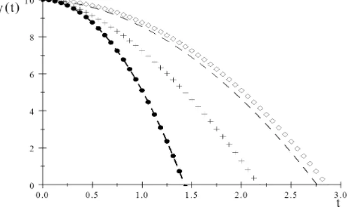
A further integration of Eq. (15) gives the solu-tion for the height of the center of mass of the drop, satisfying the initial conditiony(0) =h(Fig. 1).

y(t) =h− gm

2

o

2b2_{(−λ+ 1)}−

gm2

2b2_{(λ+ 1)}+

gmλ+1

o m

−λ+1

b2_(−λ2_{+ 1)} .

For the case without friction(λ= 1)this result se-ems to diverge, but we can see that it is not so.

First we rewrite Eq. (28) as

y(t) =h−gm

2

o

2b2





1− 2m λ₋1

o m− λ+1 (λ+1)

(−λ+ 1) 

−

gm2

2b2_{(λ+ 1)}.

(28) We define

∆1= 1− 2mλ₋1

o m− λ+1 (λ+1)

(−λ+ 1) , (29)

where it is necessary to take the limit λ → 0. Using l’Hopital rule again, we obtain

lim

x→1∆1 =

2_dλd (m

λ₋1

o m− λ+1 (λ+1)

)

d

dλ(−λ+ 1)

⌋λ=1 (30)

=−2 d

dλ

( (mo m

)λ−1

λ+ 1 )

⌋λ=1.

Figura 1 - Accretion proportional to time mo = 1 × 10−4_,

b = 9.1, free fall(·−),λ = 1.3 (××),λ = 1.5 (−−), λ = 1.8 (♦♦).

Using

d dxa

u _=au_lnadu

dx,

we can write

lim

x→1∆1 = 2

[

(λ+ 1)(mo m

)λ−1

ln(mo m

) +(mo

m

)λ−1

(λ+ 1)2

]

λ=1

(31)

= ln ( _m

mo

)

− 1 2.

On the other hand, if we define

∆2=

gm2

2b2_{(λ+ 1)}, (32)

it is evident that

lim

λ→1∆2= gm2

4b2 . (33)

Using Eqs. (32) and (34) we get

lim

λ→1y(t) =h− gm2

o

2b2

( ln

(_m

mo

)

− 1 2

)

− gm

2

4b2

(34)

=h− gm

2

o

2b2 ln

(_m

mo

)

− gmo 2b −

gt2

4 .

The particle of constant mass in free fall is obtained expandingln(_mom ), that is

ln (_m

mo

) = ln

( 1 + bt

mo

)

≈ bt

mo −

1 2

( _bt

mo

)2

.

(35) Then

y(t) =h− gm

2

o

2b2

(

bt mo −

1 2

( _bt

mo

)2)

− gmo 2b −

gt2

4

(36)

=h− gt

2

2 .

The expected result (Fig. 2).

4.

Accretion proportional to the surface

of the drop

Now we make the assumption that

dm

dt =α4πr

2_{. (37)}

Then the equation of motion for this case is

dv dt +

1

m

(

α4πr2)

v =−g. (38)

The assumption, Eq. (38), is equivalent to the hy-pothesis that the radius of the drop grows linearly with time, since

m =ρ4π

3 r

3_{, (39)}

and then

dm

dt =ρ4πr 2dr

dt. (40)

Therefore r(t) = ro+αt implies that dr_dt = α, and we obtain the usual assumption that mass grows proportionally to the surface of the drop.

Our equation of motion is then

dv dt +

3vα ro+αt

=−g. (41)

This differential equation can be solved by the same method used for the case of accretion proportional to time, and the solution with the initial condition

v(0) = 0 is

v =− g 4α

(

r− r

4

o

r3

)

. (42)

In the formal limitmo → 0, or ro → 0, r = αt and then we obtain

v(t) = gt

4; (43)

as we mentioned previously, it is a strange result. With the binomial theorem we can write this solu-tion as

v =− g 4α

[

ro+αt−ro

(

1− 3αt

ro

+· · ·

)]

,

(44) obtaining the free fall case,v =−gt, asα→0.

An integration of Eq. (44), with the initial condition

y(0) =h, gives (Fig. 3)

y(t) =h− g 8α2

[

(ro+αt)2+

r4

o

(ro+αt)2 −2r_o2

]

.

(45) Again, an expansion with the binomial theorem to second order intshows that we can obtain the free fall case asα →0.

Figura 3 - Accretion proportional to the surface of the drop:

ro = 1× 10−4_{, free fall (}·−),α = 1×10−4 ₍××),α = 1×10−3₍−−),α= 0.4 (♦♦).

5.

Accretion proportional to the surface

times the velocity

The assumption that

dm

dt =−β4πr

2_{v, (46)}

seems more natural if we notice that it is equivalent to assuming that

r(t) =ro+β(h−y(t)). (47) That is, fromm(t) = m(r(y(t))) =ρ4₃πr3 _we

find that

dm

dt = ρ4πr 2dr

dy dy

dt =−β4πr

2_{v. (48)}

Therefore our equation of motion is now the non linear equation

dv dt −

3βv2 ro+β(h−y(t))

=−g. (49)

This equation can be transformed with the identity

dv dt =

dv dr

dr

dt =−βv dv dr = −

1 2β

d(

v2)

dr . (50)

Then the equation of motion is

d(v2₎

dr +

6v2

r =

2g

β . (51)

Now we have a differential equation for v2 _{of the}

same type we have solved before, and the solution, with the initial conditionv(0) = 0, is

v2= 2g 7β

[

r− r

7

o

r6

]

. (52)

We can show with the binomial theorem that this solution reduces to the free fall case asβ →0.

v2₌ 2g

7 [

(ho−y)−

(ro_β)7

(ho−y)6

]

. (53)

Here h0is defined by

ho=h+

ro

β. (54)

Then it is obvious that

dy

dt =v =−

√ 2g

7 √

(ho−y)7−(ro_β)7

(ho−y)3

, (55)

and in order to obtainy(t)we have to solve the integral

t= −

√ 7 2g

∫ y

h

(ho−y´)3dy´

√

(ho−y´)7−(ro_β)7

. (56)

From this equation it is easy to obtain the formal limitro →0,considered by some authors [11]. In this caseho=hand Eq. (56) becomes

t=−

√ 7 2g

∫ y

h

(h−y)−12_{dy´, (57)}

which after integration and some simplifications results

y=h− gt

2

14. (58)

This result implies that

v = gt

7, (59)

that as we mention before, is strange.

This integral is not immediate and it is convenient to definezo = ro_β and z´= ho−y, in order to trans-form the integral to the trans-form

t= √

7 2g

∫ z

zo

´

z3_dz′ √

´

z7_−z7

o

. (60)

We need another change of variable

θ = z

7

z7

o

−1, (61)

so that we have now the integral

t= √

7 2g

√_z o

7 ∫ θ

0

´

θ−1

2

( 1 + ´θ)

−3

7

dθ,´ (62)

This integral is found in standard tables [12] and is given as

t= √

2zo

7g θ 1 22F1

[₃

7, 1 2,

3 2,−θ

]

, (63)

where2F1 is the hypergeometric function. In terms of the original variables we have

t= v u u t2

(

ro β

)

7g

(

(ho−y)7

(_β

ro

)7

−1 )12

×

2F1

[ 3 7,

1 2,

3 2,−

(

(ho−y)7

(_β

ro

)7

−1 )]

, (64)

that with a Taylor expansion aroundy=hresults in

t=−

√ 2

g (h−y) 1

2 ₊ (h−y) 3 2

√_2g

(_β

ro

) +

(h−y)52

√_32g

(_β

ro

)2

+O(h−y)72_{. (65)}

Finally, inverting this series we find

(h−y)12 ₌₋

√_g

2t−

g32

4√2 (_β

ro

)

t3−

7g52

32√2 (_β

ro

)2

t5+O(t)7, (66)

which after squaring givesy(t)(Fig. 4) as

y(t) =h−g 2t

2

−g

2

4 (_β

ro

)

t4+O(

t6)

. (67)

This time it is obvious that we get the free fall case as β→0.

Figura 4 - Accretion proportional to the surface times the ve-locity: ro = 1 × 10−4_{, free fall (}·−), β = 0.5 (××),

6.

Conclusions

We have solved in a general way the problem of the motion of a falling drop whose mass grows by accretion according to a specific law of accretion. We have consi-dered three specific laws of accretion, and have solved the problem by Newtonian methods. Then we had to apply a generalization of Newton’s second law, which we took as the Eulerian formulation of the equation of motion for a continuum. Specifying clearly the hy-pothesis that lead to the particular equation of motion, these examples were solved to the point of getting the path of the center of mass of the falling drop, which is the aim of the Newtonian method. As a check of the solution obtained, we obtained in all cases the correct limit of a constant mass particle in free fall and that of a particle falling with friction linear in the velocity.

Appendix

The natural generalization of Newton´s second law for a continuum is given by the Lagrangian description, since a small part of this continuum, a “particle” of constant mass, is followed through its motion under the action of external forces, the body force and the surface force given by a surface integral of the stress tensor.

Then the equation of motion in this description is

ρdv

dt =ρfb+∇ ·

←→_{T ,}

where d_dtv is the total derivative, also called material derivative, given by

dv

dt = ∂v

∂t + (v· ∇) v.

Then

ρdv dt =ρ

∂v

∂t +ρ(v· ∇) v.

The term(ρv· ∇) vcan be developed with the aid of the tensor identity

∇ ·(ρvv) = (ρv· ∇) v + v (∇ ·ρv),

and the continuity equation for conservation of mass in a given volumen,

∂ρ

∂t +∇ ·ρv = 0.

Thus

(ρv· ∇) v =∇ ·(ρvv) + v∂ρ

∂t .

Then

ρdv dt =ρ

∂v

∂t+v ∂ρ

∂t+∇·(ρvv) =

∂(ρv)

∂t +∇·(ρvv) .

Finally, the equation of motion for matter in a given volume is

∂(ρv)

∂t =ρfb+∇ ·

(←→

T −ρvv),

which is the Eulerian description of motion, the last term representing the momentum flux.

References

[1] K.S. Krane, Am. J. Phys.49, 113 (1981).

[2] M.S. Tiersten, Am. J. Phys.37, 82 (1969).

[3] L. Prandtl and O.G. Tietjens,Fundamentals of Hydro and Aerodynamics (Mc. Graw Hill, New York, 1934, Dover, New York, 1957), p. 233.

[4] G.W. Housner and D.E. Hudson, Applied Mechanics Dynamics (Van Nostrand, New York, 1959), 2nd ed. [5] R. Aris, Vector, Tensor and the Basic Equations

of Fluid Mechanics (Prentice Hall, Englewood Cliff., 1962. Dover, New York, 1989), p. 102.

[6] G. del Valle, I. Campos and J.L. Jimenez, Eur. J. Phys.

17, 253 (1996).

[7] I. Campos, J.L. Jimenez and G. del Valle, Eur. J. Phys.

24, 469 (2003).

[8] J.L. Jimenez, G. Hern´andez, I. Campos and G. del Valle, Eur. J. Phys.26, 1127 (2005).

[9] A. Sommerfeld, Mechanics (Academic Press, New York, 1964), p. 241 problem 1.6 and p. 256 .

[10] S.T. Thornton and J.B. Marion,Classical Dynamics of Particles and Sistems (Thomson Learning, Belmont, 2004), p. 385 problem 9.56, 5th ed.

[11] G.R. Fowles and G.L Cassiday, Analytical Mechanics

(Thomson Brooks/Cole, Belmont, 2005), p. 320 pro-blem. 7.23, 7th ed.