Analytic solution to the motion of mass-spring oscillator
subjected to external force
(Solu¸c˜ao anal´ıtica para o movimento de um oscilador massa-mola sujeito a uma for¸ca externa)
Youtian Zhang
1Department of Physics, Nanjing University, Nanjing, China
Department of Electrophysics, National Chiao Tung University, Hsinchu, China Recebido em 19/7/2015; Aceito em 31/8/2015; Publicado em 12/12/2015
The simple harmonic vibration, damping vibration and forced vibration of an oscillator attached to the massless spring are always discussed in general mechanics courses. In this article, we focus on the heavy-spring conditions. We first investigate the general situation where both viscous resistance and applied force are con-sidered under the perspective of the renormalization group theory. Then we use analytic method to study the damped oscillation of an oscillator attached to the heavy spring, where renormalization method fails to work.
Keywords: mass-spring oscillator, damping vibration, forced oscillation.
A vibra¸c˜ao harmˆonica simples, o amortecimento de vibra¸c˜oes e a vibra¸c˜ao for¸cada de um oscilador ligado a uma moal sem massa s˜ao sempre discutidos em cursos gerais de mecˆanica. Neste artigo, vamos nos concentrar nas condi¸c˜oes de mola com massa. N´os primeiro investigamos a situa¸c˜ao geral em que tanto a resistˆencia viscosa e a for¸ca aplicada s˜ao consideradas sob a perspectiva da teoria do grupo de renormaliza¸c˜ao. Ent˜ao, n´os usamos um m´etodo anal´ıtico para estudar a oscila¸c˜ao amortecida de um oscilador ligado a uma mola com massa, em que o m´etodo de renormaliza¸c˜ao n˜ao funciona.
Palavras-chave: oscilador massa-mola, vibra¸c˜ao amortecida, oscila¸c˜ao for¸cada.
1. Introduction
An oscillation is a common but very important phe-nomenon in the physical world. If a physical quantity is displaced from the equilibrium a little, linear negative feedback may then lead to an oscillation. A familiar ex-ample is a simple harmonic oscillator. Also, damping vibrations and forced vibrations of an oscillator are nor-mally focused [1]. The mass of the spring is neglected in models. However, the mass of the spring is unnecessar-ily neglected as to studying mass-spring system itself. In this article we try to solve the mass-spring system where the mass of the spring is not negligible.
In 1979, Weinstock studied the normal modes of the oscillator motion for the oscillator attached to a heavy spring by virtue of the Stieltjes integral [2]. In 1994, da Silva obtained the normal frequencies of elas-tic oscillations of a parelas-ticle suspended on a spring of non-negligible mass again under the perspective of the renormalization group theory [3]. A continuous spring can be regarded as a chain of many small springs cou-pling an equal amount of small masses. Then mapping process is repeated by associating two consecutive small
springs into a single one. At last, only the boundary effect matters. JM Nunes dealt with the problem only for the simplest situation, without the friction and ap-plied force, thus the advantage of this method does not emerge in this case. In fact, we can not only find out the normal frequencies in the conservative system, but also obtain the specific equation of motion when external forces are acted on.
In the next sections, we first explore the most gen-eral condition, a forced vibration with viscous resis-tance, using the renormalization method. Then we deal with a special case analytically where the renormaliza-tion method fails to work. We investigate the orthogo-nality of the solutions of the PDEs in base set, and then obtain the motion of the damping oscillator attached to a heavy spring.
2.
The
forced
mass-oscillator
with
damping
Hang an uniformly distributed spring with massm ver-tically. The top side is fastened to stable fixture and
1E-mail: [email protected].
the bottom side concatenate an object with massM as oscillator. The free length of spring is L and the stiff-ness coefficient isk. To be discretized, the heavy spring is viewed as a series of small non-massN equal springs and each small spring is coupled with a concentrated object with mass m/N. The natural length and elastic constant (labeled by s) of each small spring are L/N
and s = kN respectively. The damping on the oscil-lator M can be calculated as −bvM if the velocity of oscillator isvM and damping coefficient isb. Besides, a time-dependent forcef(t) is applied on the oscillator.
Figure 1 - A discretization model. The heavy spring with natu-ral lengthL, massm and stiffness coefficientkis divided intoN
small springs coupled with concentrated objects.
The positions of objects are denoted by
xn(n = 0,1, ..., N), then equations of motion can be set up as
x0= 0, (1a)
m N
d2
dt2xn=s(xn−1−2xn+xn+1)+
m
Ng (1≤n≤N−1), (1b) M d
2
dt2xN =−s(xN −xN−1−
L N)+ M g−bd
dtxN+f(t). (1c)
We can eliminate the constant terms derived from grav-ity in the Eq. (1) by changing the coordinates appro-priately. So that we can use newly defined coordinates (un =xn−NnL−ngs [M+(2N−n−1)2mN], n= 0,1, ..., N) to describe the motion (da Silva proposed a way to ap-proach these newly defined coordinates [3]). The
equa-tions with new coordinates are written as follows,
u0= 0, (2a)
m N
d2
dt2un=s(un−1−2un+un+1)
(1≤n≤N−1), (2b)
M d
2
dt2uN =−s(uN −uN−1)−b
d
dtuN +f(t). (2c)
If we denote
˜
f =1
sF[f(t)] =
1
N k
∞
∫
−∞
f(t)e−iωtdt,
and
Un=F[un(t)] =
∞
∫
−∞
un(t)e−iωtdt(n= 0,1, ..., N),
then the Eq. (2) can be Fourier transformed as
U0= 0, (3a)
cUn =Un−1+Un+1 (1≤n≤N−1), (3b)
CUN =UN−1+ ˜f , (3c)
withc= 2(1−2mωN22k) andC= 1 +iωb−M ω 2
N k .
By Eq. (3), we get c2U2n = c(U2n−1+U2n+1) =
U2n−2 + 2U2n+U2n+2 and cCUN = cUN−1+cf˜ =
UN−2+UN +cf˜. We combine two small springs into a bigger small spring. That is, with this mapping pro-cess, the previous (2n−1)th and (2n)th springs now
become the nth bigger small spring. The new Fourier transformed position function ofnth spring is denoted byUn andUn=U2n. So we have
U0= 0, (4a)
(c2−2)Un =Un−1+Un+1, (4b)
(cC−1)UN
2 =UN2−1+c ˜
f . (4c) Comparing Eq. (4) and Eq. (3), the equations change regularly2 after the process of combining two
consecu-tive small springs into bigger spring. So we repeat the combination to renormalize. If we set N = 2p, then after pth repeat, Eq. (4c) finally becomes C(p)U
1 =
U0+ ˜f p−1 ∏
κ=0
c(κ). U0= 0 and the position function of the
oscillator is
uoscillator(t) =F−1[U1(ω)] =
1 2π
∞
∫
−∞
˜
f
p−1 ∏
κ=0
c(κ)
C(p) e iωtdω.
(5) The next thing to do is to find out the iteration
valueC(p)and p−1 ∏
κ=0
c(κ). Comparison between Eqs. (3)
2After each iteration, the coefficients of left terms in Eqs. (4b) and (4c) update toc(l+1)=c(l)2−2 andC(l+1)=c(l)C(l)−1 from
and (4) gives c(1) = c2 −2 and C(1) = cC −1, so 2C(1)−c(1) =c(2C−c) and more generally,
2C(p)−c(p)= (2C−c) p−1
∏
κ=0
c(κ).
Introduce γ and let c ≡ 2 cosγ. c(p) and p−1
∏
κ=0
c(κ) are easily accessible with this variable substitution, i.e.
c(p)= 2 cos 2pγ, p−1 ∏
κ=0
c(κ)= sin 2 pγ
sinγ . Finally,
C(p)= 1 2[
sin 2pγ
sinγ (2C−c) + 2 cos 2
pγ].
c≡2 cosγ= 2(1−2mωN22k). Notice thatN≫1, soγ≪1 andγ= sinγ= ω
N
√m
k.By Eq. (5),
⌋
uoscillator(t) = 1
2π
∞
∫
−∞
2 sin(ω√m k) ˜f
sin(2pγ)(2C−c) + 2 sinγcos(2pγ)e iωtdω
= 1 2π ∞ ∫ −∞ ∞ ∫ −∞
f(t)e−iωtdt
iωb−M ω2+ cot(ω√m k)ω
√
kme
iωtdω.
(6)
Thenxoscillator(t) =uoscillator(t) +L+ (M+m2)gk (neglect−2mgkN because ofN ≫1) due touN =xN−L−N gs [M+ (N−1)m
2N]. It’s the motion equation of the oscillator with consideration of mass of spring, external forces including damping, gravity and applied time-dependent force.3 But one thing to note here is that f(t) can not be 0 or the
solution vanishes. We deal with this condition in following part.
In fact, if g(t) ≡ 21π
∞
∫
−∞
1 iωb−M ω2+cot(ω√m
k)ω √
kme
iωtdω(≡ 1 2π
∞
∫
−∞
G(ω)eiωtdω),4 the motion equation of the
oscillator can be given by the convolution of f(t) and g(t), i.e. uoscillator(t) = f(t)∗g(t). From the following
discussion, we will know that the frequencies which satisfyiωb−M ω2+ cot(ω√m k)ω
√
km= 0, which make G(ω) divergent and lead to resonance, are exactly eigenvalues in no applied force condition (see Eq. (9)).
⌈
3.
No applied force condition
Since we can no longer use renormalization method for no applied force condition, we then use mathematical physics equations to study this problem. Adopt appro-priate coordinates as introduced before, and the
prob-lem can be analytically described as follows.5
utt−kL 2
m uxx= 0 (t >0, x∈[0, L)),
u(0, t) = 0, ux(L, t) =−
M
kLutt(L, t)− b
kLut(L, t), u|t=0=φ(x),
∂u ∂t t=0
=ψ(x).
(7)
We consider using method of separation of vari-ables to solve this equation and we take u(x, t) =
X(x) exp(−iµL
√ k
mt) as the ansatz. The equations
3Notice that ∞∫
−∞
∞
∫
−∞
f(t)e−iωtdt
iωb−M ω2+cot(ω√m k)ω
√ kme
iωtdω = −∞∫
∞
∞
∫
−∞
f(t)e−i(−ω)tdt
i(−ω)b−M(−ω)2+cot((−ω)√m k)(−ω)
√ kme
i(−ω)td(−ω), so
∞ ∫ −∞ ∞ ∫ −∞
f(t)e−iωt
dt
iωb−M ω2+cot(ω√m k)ω
√ kme
iωtdω= ∞∫
−∞
∞
∫
−∞
f(t)eiωtdt
−iωb−M ω2+cot(ω√m k)ω
√ kme
−iωtdωandu
oscillator(t) is pure real.
4By lim
m→0cotω
√
m k =
√
k
m/ω, we have limm→0G(ω) = iωb−M ω1 2+k, which is consistent with the transfer functionG(s) =M s2+1bs+k for standard 2nd order mass/spring/damper system by Laplace transformation. [4] There is also another conclusion if we add one more expansion term in cotx (cot ≃ 1x −x3 − x453 +...within radius of convergence), lim
m→0cotω
√
m k =
√
k m/ω−
1 3ω
√
m k, hence lim
m→0
G(ω) = 1
iωb−M ω2+k−1 3mω2
. In no viscous case (b= 0), revised natural circular frequency for spring mass system isω= k
M+m/3
where spring’s effective mass ism/3, [5] which can be obtained from lim
m→0G(ω) =
1
−(M+m/3)ω2+k.
5Take infinitesimal spring with length dx, stiffness coefficient kL
dx and mass
dx
Lm. The position deviation of infinitesimal spring from
equilibrium is denoted by du. Then motion equation of the infinitesimal spring can be given by ∂(
kL
dxdu)
∂x dx=dLxm·d
2u
above then become
X′′(x) +µ2X(x) = 0, (8a)
X(0) = 0, (8b)
X′(L) = (iµ√b
km +µ
2M L
m )X(L), (8c) X(x) =φ(x), (8d)
−iµL
√
k
mX(x) =ψ(x). (8e)
By Eqs. (8a) and (8b), we substitute X(x) = sinµx
into Eq. (8c) and get the eigenvalue equation
cotµL=i√b
km +µ M L
m . (9)
We set that Xp(x) and Xq(x) are different solutions from the base set. To obtain expansion coefficients from initial conditions (8d) and (8e), we first derive the or-thogonality relation between bases Xp(x) and Xq(x) within the boundary condition (8c). According to Eqs. (8a) and (8c), we have
Xp′′(x) +µ2pXp(x) = 0, (10a)
Xp′(L) = (iµp
b
√
km+µ
2 p
M L
m )Xp(L), (10b) Xq′′(x) +µ2qXq(x) = 0, (10c)
Xq′(L) = (iµq
b
√
km +µ
2 q
M L
m )Xq(L). (10d)
⌋
Calculate Eq. (10b) ×Xq(L)−Eq.(10d)×Xp(L) and we get
M L m (µ
2
p−µ2q)Xp(L)Xq(L) +i(µp−µq)
b
√
kmXp(L)Xq(L)
=Xq(x)Xp′(x) L 0 −
∫ L
0
Xp′(x)Xq′(x)dx−Xp(x)Xq′(x) L 0 +
∫ L
0
Xp′(x)Xq′(x)dx
= ∫ L
0
Xq(x)Xp′′(x)dx− ∫ L
0
Xp(x)Xq′′(x)dx
=−µ2p
∫ L
0
Xq(x)Xp(x)dx+µ2q ∫ L
0
Xp(x)Xq(x)dx.
(11)
From Eq.(11) we eventually reach the following equality under the boundary condition (8c),
∫ L
0
Xq(x)Xp(x)dx+ [
M L m +i
b
(µp+µq)
√
km
]
Xp(L)Xq(L) = 0. (12)
Eq. (12) shows that the solutions in the base set are generalized orthogonal [6]. The squared norms (denoted by
N2) of the eigenfunctions can be calculated as
N2[Xp(x)] = ∫ L
0
Xp2(x)dx+ [
M L m +i
b
2µp
√
km
]
Xp2(L)
Xp(x)=sinµpx
===========
Eq.(10b)
L
2 −
1 4µp
sin 2µpL+
cosµpLsinµpL 2µp
+M L
2m sin
2
µpL
= L
2 +
M L
2m sin
2µ pL.
(13)
So the solution to the Eq. (7) can be written asu(x, t) =∑
nAnsinµnxexp(−iµnL √
k
mt); the expansion coefficients
Anare determined byφ(x) andψ(x) collectively. We then expandφ(x) andψ(x) based on the orthogonality relation (12): φ(x) =∑
nPnsinµnx, ψ(x) =−i∑nµnL √
k
mQnsinµnxwhere
Pn= ∫L
0 φ(x) sinµnxdx+ [
M L m +i
b 2µn
√
km ]
φ(L) sinµnL
N2[X n(x)]
, (14a)
Qn= ∫L
0 i µnL
√m
kψ(x) sinµnxdx+ [
M L m +i
b 2µn
√
km ]
i µnL
√m
kψ(L) sinµnL
N2[X n(x)]
LetAn=αnPn+βnQn, then
φ(x) =∑ n
(αnPn+βnQn) sinµnx, (15a)
√
m
kψ(x) =−i
∑
n
µnL(αnPn+βnQn) sinµnx. (15b)
Comparing Eq. (15a) +χEq. (15b) withφ(x) =∑
nPnsinµnx,χ√mkψ(x) =−iχ∑nµnLQnsinµnx, we get
Pn[(αn−1)−iχµnLαn] +Qn[βn−iχµnL(βn−1)] = 0. (16) Hence,αn=1−iχµ1 nL andβn = 1−αn=
−iχµnL
1−iχµnL. FinallyAn can be given as
An= ∫L
0[φ(x) +χ
√m
kψ(x)] sinµnxdx+ [ M L
m +i b 2µn
√
km][φ(L) +χ
√m
kψ(L)] sinµnL
N2[X
n(x)](1−iχµnL)
, (17)
where χ is determined by the initial conditions both φ(x) and ψ(x).6 For the simple but most common case, if
ψ(x) = 0,i.e. ∂u∂t
t=0= 0, we haveχ= 0 (henceAn=Pn). According solutions satisfy Eqs. (7) whent >0.
⌈
The eigenvalue equation reveals as cotµL=i√b km+
µM Lm (eigenvalueµwon’t be 0). Notice that−µis also eigenvalue ifµis eigenvalue. The corresponding expan-sion coefficients have the relationP(−µ) =−P(µ) and
Q(−µ) = −Q(µ) due to the Eq. (14). Considering sin(−µx) =−sinµx,
∑
n
Pnsinµnx= ∑
Re(µn)>0
[Pnsinµnx+Pnsinµnx] =
∑
Re(µn)>0
[Pnsinµnx+c.c.], (18a)
−i∑
n
µnL √
k
mQnsinµnx=
−i[ ∑
Re(µn)>0
[µnL √
k
mQnsinµnx]−c.c.]. (18b)
Eq. (18) verifies that bothφ(x) andψ(x) are pure real when ansatz
u(x, t) =∑ n
Ansinµnxexp(−iµnL √
k mt),
is taken. Of course u(x, t) = ∑
Re(µn)>0
[Ansinµnx
exp(−iµnL √
k
mt) +c.c.] is also pure real. We can
ob-tain two types of independent eigen-vibration modes
from this result. Letµn =ξn−iζn7, then
sinµnxexp(−iµnL √
k mt) =
(sinξnxcoshζnx−icosξnxsinhζnx)×
exp(−ζnL √
k
mt)[cos(ξnL
√
k
mt)−isin(ξnL
√
k mt)]
= [sinξnxcoshζnxcos(ξnL √
k mt)−
cosξnxsinhζnxsin(ξnL √
k
mt)] exp(−ζnL
√
k mt)− i[cosξnxsinhζnxcos(ξnL
√
k mt)+
sinξnxcoshζnxsin(ξnL √
k
mt)] exp(−ζnL
√
k mt).
The two types of independent vibration modes are given
6Ifφ(x) andψ(x) are dependent, to be more precise,P
n=Qn,χcan be any value. In this case, either Eq. (14a) or Eq. (14b) can be equally used to calculate the expansion coefficientAn, and don’t bother to introduceχ.
7It’s hard to find allµs analytically from cotµL=i b √
km+µ M L
m but we can use perturbation to investigate since imaginary part in RHS of eigenvalue equation b
√
km is feeble in generally underdamping conditions. The zero-order approximation,µ
(0)tanµ(0)L= m M L for zero friction situation (b= 0), is discussed in previous work [2]. Obviously, solutions are real numbers and come in pairs (−µ(0)is
also solution ifµ(0)satisfies zero-order eigenvalue equation). Perturbation calculation shows the first order modification is negative pure
imaginary number and the paired zero-order eigenvalues±µ(0)share the same first order modification. It coincides with the previous
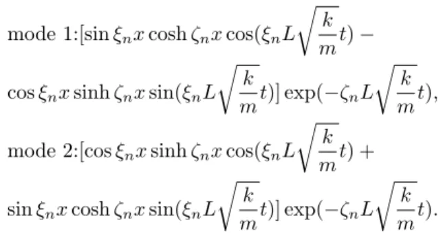
by8
mode 1:[sinξnxcoshζnxcos(ξnL √
k mt)−
cosξnxsinhζnxsin(ξnL √
k
mt)] exp(−ζnL
√
k mt),
mode 2:[cosξnxsinhζnxcos(ξnL √
k mt) +
sinξnxcoshζnxsin(ξnL √
k
mt)] exp(−ζnL
√
k mt).
The oscillator (x =L) vibrates with damped amplitude (as is shown in Fig. 2) in both types of modes, which is reasonable.
Figure 2 - Let t/τ be dimensionless with τ = √m
k/ξnL, the eigen-vibration mode of the oscillator can be plotted under two cases withζn/ξn= 0.1 andζn/ξn= 0.2. The oscillator vibrates with damped amplitude.
For zero-friction case (b= 0), the solutions to eigen-value equation cotµL=i√b
km+µ M L
m are pure real,i.e.
ζ= 0. Then two types of vibration modes become9
mode type 1: sinξnxcos(ξnL √
k mt),
mode type 2: sinξnxsin(ξnL √
k mt).
Summarize the result: the solution to Eq. (7) is
u(x, t) =∑
nAnsinµnxexp(−iµnL √
k
mt) where eigen-valueµn is given by Eq. (9). Expansion coefficientAn and squared norms are given by Eqs. (17) and (13).
4.
Conclusion
In this article, we detailedly studied the vibration of spring oscillator when the mass of the spring can’t be neglected. Damped oscillation and forced vibration are especially focused. For general condition, oscilla-tion with fricoscilla-tion and applied force, renormalizaoscilla-tion method is employed to obtain the equation of the mo-tion. Renormalization method shows superiority when applied force f(t) exerts on the oscillator. We also in-vestigate the damping vibration without applied force with theory of partial differential equations. For given boundary condition, the generalized orthogonality of base set is studied. We discussed the characters of the eigenvalue and the expansion coefficient and the discus-sions verified the validity of the solution.
References
[1] L.D. Landau, E.M. Lifshitz, Mechanics: Volume 1 (Course Of Theoretical Physics) (Butterworth-Heinemann, Oxford, 1976).
[2] R. Weinstock, American Journal of Physics 47, 508 (1979).
[3] J.M N. da Silva, American Journal of Physics62, 423 (1994).
[4] S.M. Shinners,Modern Control System Theory and De-sign (John Wiley & Sons, New York, 1998).
[5] Y. Yamamoto, Journal of Sound and Vibration 220, 564- (1999).
[6] Tyn Myint-U,Partial Differential Equations of Math-ematical Physics (North-Holland, New York, 1973). [7] M.S. Santos, E.S. Rodrigues and P.M.C. de Oliveira,
American Journal of Physics58, 923 (1990).
8To get a more detailed understanding of exp(−ζ
nL
√
k
mt), we use cotz≃ 1z−z3−z
3
45+...again within the radius of convergence.
The first-order approximation of cot(ξn−iζn) in eigenvalue equation gives thatζξnn =√b/2M
k mξnL
, so the dumping factor is exp(−bt/2M),
which is the same as the damping factor of common damped oscillators. [1] The second-order approximation shows that the dumping factor is exp[−bt/2(M+m/3)].
9With tanξ
nL=M ξmnL, the frequencyξnL
√
k
m degrades if we neglect the mass of the spring,i.e.m→lim0ξnL
√
k m=
√
k
M for allξn.
Thus, many degrees of freedom are reduced in one body problem,ω=
√