Flow Simulation in Engine Cylinder with Spring Mesh

ISSN 1546-9239

© 2008 Science Publications

Corresponding Author: A.R. Noorpoor, Department of Automotive Engineering, Iran University of Science and Technology, Narmak, Tehran, Iran

Flow Simulation in Engine Cylinder with Spring Mesh

M.H. Shojaeefard and A.R. Noorpoor

Department of Automotive Engineering,

Iran University of Science and Technology, Narmak, Tehran, Iran

Abstract: This investigation presents results from numerical simulation of the air flow in Spark Ignition Engine (SI engine) cylinder. Accurate modeling of the flow in cylinder is a key part of successful combustion simulation. The most usual numerical method in Computational Fluid Dynamics (CFD) is finite volume. In this investigation an important, common fluid flow patterns in CFD simulations, namely, Tumble motion typical in automotive engines and RNG k-ε turbulence model were used. The air flow in a two-valve engine cylinder during 720 degree of crank angle was investigated by using a CFD code which is basis on finite volume and codes which were written in visual C++ environment. Dynamic Mesh and Moving Boundary capability were used for this model. The comparison results with previous researches results, Kiva-3v and PIV experimental, show good agreement.

Key words: Moving boundary, internal combustion engine, flow field

INTRODUCTION

With the advent of more powerful computers, now mathematical models are increasingly accepted as design and optimization tools for engine development. To accepting a mathematical tool for engine design, it is necessary to validate the model results by experimentation.

Developments in engine simulation technology have made the virtual engine model a realistic proposition[1]. Today the usage of CFD codes has developed and these codes can be used to engine simulation[2-3]. The use of CFD on engine development programs has enabled significant time and cost savings to be made in the design and development of engine combustion engine system. Accurate modeling of the flow in cylinder is a key part of successful combustion simulation.

A mixture formation in an SI Engine is a complex phenomenon that is involved by large number of design and operating variables, so it is necessary to understand the in-cylinder flow characteristics for reliable designing, fuel efficient and low emission engine. Also the sensitivity of the flow distribution turns back to the shape of intake port and combustion chamber so is gotten higher efficiency with better design[4-6].

For many of the automotive components, there is an ideal pattern of flow that engineers were trying to create. In the flow within a cylinder, there are two types

of motion: swirl flow commonly found in diesel engines and tumble flow commonly found in gas engines. In both cases, rotational motion occurs about an axis, though the position of the respective axis is different. In the case of swirl flow, the axis is more or less coincident with the cylinder axis[7].

In the case of tumble, the rotation axis is perpendicular to the cylinder axis and more complex, thus making tumble flow more difficult to control than swirl flow.

In order to generate swirl or tumble motion, fluid enters the combustion chamber from the intake ports. The kinetic energy associated with this motion is used to generate turbulence for mixing of fresh oxygen with evaporated fuel. The more turbulence generated lead to the better mixture of air and fuel. However, too much tumble (or swirl) can displace the flame used to ignite the fuel, cause irregular flame propagation, or result to less fuel combustion[8].

As such, a balanced generating swirl or tumble flow must be achieved and not displacing the flame. A controlled flow motion is used to get stable and reproducible conditions at each engine cycle.

NUMERICAL SOLUTION

directions of cartesian coordinate, one energy equation, k equation and ε equation organize the seven equations for flow simulation[7].

( )

div u 0

t

∂ρ

+ ρ =

∂ (1)

(

)

p Du

S

Dt x y z

∂τ

∂ − + τ ∂τ

ρ = + + +

∂ ∂ ∂ (2)

(

)

xy zy

My

p Dv

S

Dt x y z

∂ − + τ

∂τ ∂τ

ρ = + + +

∂ ∂ ∂ (3)

(

)

Dt x y z

∂τ ∂ − + τ

∂τ

ρ = + + +

∂ ∂ ∂ (4)

( )

(

)

(

)

(

)

(

)

(

)

(

)

(

)

(

)

(

)

(

)

xy yy zy xz

yz zz E u u u DE div pu

Dt x y z

v v v w

x y z x

w w

div k grad T S

y z

∂ τ

∂ τ ∂ τ

ρ = − + + + +

∂ ∂ ∂

∂ τ ∂ τ ∂ τ ∂ τ

+ + + +

∂ ∂ ∂ ∂

∂ τ ∂ τ

+ + +

∂ ∂

(5)

(

)

₍

₎

t

t ij ij

k k

div k U t

div grad k 2 E .E

∂ ρ

+ ρ

∂ µ

= + µ − ρε

σ

(6)

( )

₍

₎

2

1 t ij ij 2

div U div grad

t

C 2 E .E C

k k

ε

ε ε

∂ ρε µ

+ ρε = ε

∂ σ

ε ε

+ µ − ρ

(7) where 2 t k Cµ

µ = ρ

ε and ij

U E y ∂ = ∂ .

For turbulent simulation the standard k-ε model was used, also the equations coefficients were modified for impressive effect on convergence. The modified coefficients are listed in Table 1[9-10].

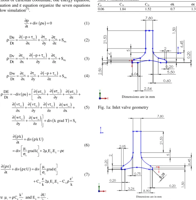
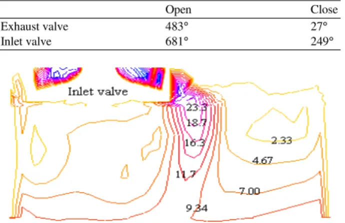
Geometry and mesh generation: Geometry dimensions of inlet and exhaust valves are shown in Fig. 1a and b. these valves and piston movement is dedicated to Y direction. The bore of combustion chamber is 0.04365m and its stroke is 0.0667m so capacity of one cylinder is 400cc. also compression ratio of chamber is 7.8.

Table 1: Modified cofficients

Cµ C1ε C2ε σk σε

0.06 1.84 1.52 0.7 1.3

Dimensions are in mm

Fig. 1a: Inlet valve geometry

Dimensions are in mm

Fig. 1b: Exhaust valve geometry

For moving parts, two valves and one piston was used two kind of mesh. The combustion chamber divided into two zones. The first one is the zone which piston moves through it and another one is the part which includes valves movement and the ports.

Fig. 2a: Different mesh type

Fig. 2b: Different mesh size

were used tetrahedral elements. This kind of mesh can expand and contract when valves are move and has spring specification.

Elements with different size were used for the valves surfaces. For instance in the curved part of the valves have used smaller elements in order to have enough accuracy when valves move down and elements expand. In Fig. 2a and b are shown difference elements in type and size.

Totally there are three methods to update the meshes of a moving boundary project:

• Smoothing • Re-meshing • Layering

Fig. 3a: Center plane

Fig. 3b: Considered plane

Fig. 3c: Chosen plane to result observation

Fig. 4a: Contours of velocity at θ = 50°

Fig. 4b: Vectors of velocity at θ = 50°

the elements just can expand and contract and there is no difference between the numbers of the layers. So spring specification in this model just is seen. Smoothing model is a useful model and it can use in a wide range of moving boundaries simulations.

Re-meshing method is after the smoothing method. In Re-meshing method generate new layers, when tetrahedral cells exist. If geometry be complicated the Re-meshing process takes a lot of time and is so expensive. An example of Re-meshing method is shown in Fig. 4. In this figure can see modified geometry with Re-meshing method.

At last, the Layering method. When there are large movements with hexahedral cells the Layering method is so suitable. Again there is an example of layering method in Fig. 5. There is the first geometry and modified geometry with layering method.

For moving parts, two valves and one piston were used 8 codes. 2 codes have written for each valve and 4 codes for piston movement by visual C++ programming language. The valve timing for exhaust and inlet crank shafts degree are written in Table 2.

Boundary conditions: Mass flow inlet is one boundary condition for this simulation in the intake port. Pressure outlet is also boundary condition in the exhaust port. The preference of this boundary condition to outflow is: if reverse flow is existed in outlet was given better convergence. The boundary condition of valves, inner surface of cylinder and piston are wall and aren’t penetrable.

Table 2: Value timing for exhaust and Inlet crank

Open Close

Exhaust valve 483° 27°

Inlet valve 681° 249°

Fig. 5a: Contours of velocity at θ = 90°

Fig. 5b: Vectors of velocity at θ = 90°

Physical properties: In this simulation air assumed as ideal gas. With this assumption the density will be variable but the other properties like viscosity and thermal conductivity will be permanent.

Solution: Create the movement of two valves and piston during 720 degree rotating of crank shaft needs. For generate the movement was used the codes which are written in visual C++ environment. These codes compile with CFD code and generate the applied movement. The valves move with constant velocity, also can use periodic velocity by modifying the codes. Piston moves with real velocity according to equation 8. In equation 8, s, θ, n and N are stroke, angel of crank shafts rotation , the ratio of piston rod length to stroke and velocity of crank shaft respectively.

V = ( sN/60)[sin + (1/2n) sin cos ]π θ θ θ (8)

RESULTS AND CONCLUSION

dimensional results are shown. In Fig. 3a, b and c two chosen plane to observe result is shown. Considered plane in top of cylinder and center plane in center of cylinder are given result figures.

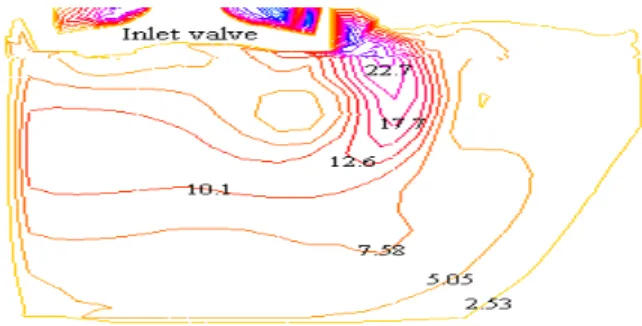
In following figures, contours and vectors of velocity in different crank angles are shown. According to Fig. 4a-9a the inlet gas velocity increases with crank angle as long as θ approach to 180° and then decreases as long as valve is closed. Velocity of gases in region near piston is proportional with piston velocity. When piston moves down, in θ = 90° and when returns, in θ = 270° the maximum content of velocity occur and in about θ = 180° minimum.

From Fig. 4b-9b the tumble in cylinder is obvious. In BDC the velocity vectors direction changes due to piston moved form. This is vivid in mention figures.

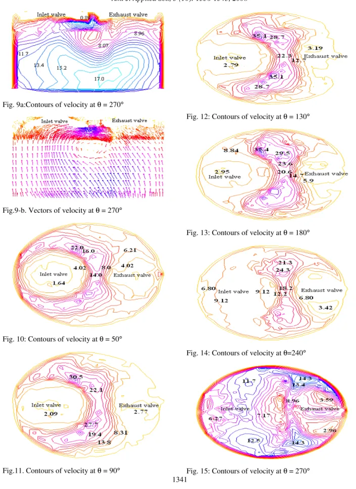
In Fig. 10-15 the velocity contours in considered plane are shown. Velocity in region under inlet valve is minimum content as long as piston moves down and maximum occur in around of it. When piston moves up velocity in region near cylinder wall is maximum value. This occurs because of piston shape.

Fig.6-a. Contours of velocity at θ = 130°

Fig. 6b: Vectors of velocity at θ = 130°

Fig. 7a: Contours of velocity at θ = 180°

Fig. 7b: Vectors of velocity at θ = 180°

Fig. 8a: Contours of velocity at θ = 240°

Fig. 9a:Contours of velocity at θ = 270°

Fig.9-b. Vectors of velocity at θ = 270°

Fig. 10: Contours of velocity at θ = 50°

Fig.11. Contours of velocity at θ = 90°

Fig. 12: Contours of velocity at θ = 130°

Fig. 13: Contours of velocity at θ = 180°

Fig. 14: Contours of velocity at θ=240°

PIV Experimental Kiva Simulation This Simulation

Fig. 16: Velocity vector in θ = 180°

PIV Experimental Kiva Simulation This Simulation

Fig. 17: Velocity vector in θ = 270°

0 180 180 180 720

Crank angle (deg)

P

re

ss

u

re

(

at

m

)

40

30

20

10

Experimental

Simulation

Fig. 18: Pressure distribution

Also experimental pressure diagram of this engine is obtained. The comparison of pressure result is indicated in Fig. 18. For simulation results was supposed same pressure for cylinder because the pressure variation in different region of cylinder is very low. High difference in combustion stroke (between θ = 280 to θ = 540°) is because of lack of combustion simulation. In other crank angle is seen good agreement.

NOMENCLATURE

ρ = Density

u, v, w = Velocity components U = Mean velocity

SM = Source term of momentum

E = Energy

SE = Source term of energy

T = Temperature p = Pressure

V = Velocity of piston s = Stroke

n = Ratio of piston rod length to stroke N = Rotation velocity of crank

k = Turbulent kinetic energy

ε = Turbulent kinetic energy dissipation θ = Crank angle

τ = Shear stress

µt = Turbulent dynamic viscosity

REFERENCES

1. Li, G., S.M. Sapsford and R.E. Morgan, 2000. CFD Simulation of a DI Truck Engine Using Vectis, SAE-01-2940.

3. P.Go. Drie and M. Zellat, 1994. Simulation of Flow Field Generated by Intake Port, Valve and Cylinder Configurations and Comparison with Measurements and Applications, SAE Paper, No. 940521.

4. Ohm, I., H. Ahn, W. Lee, W. Kim, S. Park and D. Lee, 1993. Development of HMC Axially Stratified Lean Combustion Engine, SAE Paper No. 930879.

5. Neusser, H.J., L. Spiegel, J. Ganser, 1995. Particle Tracking Velocimetry-A Powerful Tool to Shape the Incylinder Flow of Modern Multi-valve Engine Concepts, SAE Paper.

6. Hicks, R.M. and G.N. Vanderplaats, 1975. Design of Low Speed Airfoil by Numerical Optimization, SAE Paper No. 750524.

7. Das, S. and D. Chmiel, 2001. Computational and Experimental Study of In-Cylinder Flow in a Direct Injection Gasoline (DIG) Engine, 11th International Multidimensional Engine modeling User’s Group Meeting Agenda, Detroit, USA, March 4.

8. Baysal, O., 1991. Multidisciplinary Application of Computational Fluid Dynamics, winter Annual Meeting Atlanta, ASME , paper No. 129.

9. Patankar, S.V., 1980. Numerical Heat Transfer and Fluid Flow, Hemisphere Publishing Corporation, Taylor and Francis Group, New York.