Transport of short-lived species into the Tropical Tropopause Layer

(1)

www.atmos-chem-phys.net/12/6309/2012/ doi:10.5194/acp-12-6309-2012

Chemistry

and Physics

Transport of short-lived species into the Tropical Tropopause Layer

M. J. Ashfold1, N. R. P. Harris1, E. L. Atlas2, A. J. Manning3, and J. A. Pyle1,4 1_{Department of Chemistry, University of Cambridge, Cambridge, UK}

2_{Rosenstiel School of Marine and Atmospheric Science, University of Miami, Miami, Florida, USA} 3_{Met Office, Exeter, UK}

4_{National Centre for Atmospheric Science, UK}

Correspondence to:M. J. Ashfold (mja63@cam.ac.uk)

Received: 13 November 2011 – Published in Atmos. Chem. Phys. Discuss.: 6 January 2012 Revised: 1 May 2012 – Accepted: 26 May 2012 – Published: 19 July 2012

Abstract. We use NAME, a trajectory model, to

investi-gate the routes and timescales over which air parcels reach the tropical tropopause layer (TTL). Our aim is to assist the planning of aircraft campaigns focussed on improv-ing knowledge of such transport. We focus on Southeast Asia and the Western Pacific which appears to be a par-ticularly important source of air that enters the TTL. We first study the TTL above Borneo in November 2008, un-der neutral El Ni˜no/Southern Oscillation (ENSO) conditions. Air parcels (trajectories) arriving in the lower TTL (below

∼15 km) are most likely to have travelled from the boundary layer (BL;<1 km) above the West Pacific. Few air parcels

found above∼16 km travelled from the BL in the previous 15 days. We then perform similar calculations for moderate El Niño (2006) and La Niña (2007) conditions and find year-to-year variability consistent with the phase of ENSO. Under El Niño conditions fewer air parcels travel from the BL to the TTL above Borneo. During the La Niña year, more air parcels travel from the BL to the mid and upper TTL (above

∼15 km) than in the ENSO-neutral year, and again they do so from the BL above the West Pacific. We also find intra-month variability in all years, with day-to-day differences of up to an order of magnitude in the fraction of an idealised short-lived tracer travelling from the BL to the TTL above Borneo. These calculations were performed as a prelude to the SHIVA field campaign, which took place in Borneo during Novem-ber 2011. So finally, to validate our approach, we consider measurements made in two previous campaigns. The features of vertical profiles of short-lived species observed in the TTL during CR-AVE and TC4 are in broad agreement with calcu-lated vertical profiles of idealised short-lived tracers. It will require large numbers of observations to fully describe the

statistical distribution of short-lived species in the TTL. This modelling approach should prove valuable in planning flights for the long-duration aircraft now capable of making such measurements.

1 Introduction

Catalytic cycles involving bromine are known to destroy ozone in the lower stratosphere (Yung et al., 1980; Salaw-itch et al., 2005). The major sources of stratospheric bromine are currently the family of halons, which have lifetimes of up to 65 yr, and methyl bromide (CH3Br), which has a

life-time of 0.8 yr (Montzka and Reimann, 2011). However, mea-surements of these longer-lived compounds in the upper tro-posphere (e.g. Laube et al., 2008), and of subsequently pro-duced bromine monoxide in the stratosphere (e.g. Dorf et al., 2006) suggest that an additional bromine source of ∼5 ppt must exist. Various recent modelling studies (e.g. Gettelman et al., 2009; Hossaini et al., 2010; Liang et al., 2010) have shown that so-called very short-lived substances (VSLS), usually defined as having mean atmospheric lifetimes of less than 6 months, could provide a significant fraction of this ex-tra source of bromine to the sex-tratosphere.

These VSLS, including bromoform (CHBr3) and

dibro-momethane (CH2Br2), are largely emitted by macroalgae

(2)

in to the primary gateway to the stratosphere, the tropical tropopause layer (TTL) (e.g. Fueglistaler et al., 2009). A range of models suggest that emissions from Southeast Asia and the tropical Western Pacific are more likely to enter the TTL than emissions from other tropical longitudes (e.g. Levine et al., 2007; Aschmann et al., 2009; Hosking et al., 2010; Pisso et al., 2010).

There remains, however, uncertainty in each of the fol-lowing aspects of this problem: (1) the size, and the distri-bution of VSLS sources; (2) the rate and paths of transport from surface to stratosphere; and (3) the chemical and phys-ical mechanisms by which VSLS and their products are re-moved while travelling towards the stratosphere. To reduce these uncertainties remains an important goal, not least be-cause it is conceivable that each of these processes are af-fected by changes in climate over the coming century. Fur-ther motivation is provided by the introduction of additional “anthropogenic” sources of VSLS. Commercial cultivation of macroalgae has become an increasingly important part of many Asian economies, with global production growing at an average annual rate of 7.7 % since 1970 (FAO Fisheries and Aquaculture Department, 2010). In addition, the feasi-bility of using microalgae as a biofuel is receiving increasing attention (e.g. Mata et al., 2010).

As VSLS have inhomogeneous sources and short lifetimes it is unsurprising that both surface (e.g. Yokouchi et al., 2005; Butler et al., 2007; O’Brien et al., 2009; Pyle et al., 2011) and airborne (e.g. Schauffler et al., 1999; Laube et al., 2008; Hos-saini et al., 2010; Park et al., 2010) measurements of these compounds exhibit significant variability. And because ob-servations are sparse in both space and time, it is questionable how representative of the larger-scale reality any particular set of measurements might be. In this study we focus on the modelling techniques which might be used to understand ob-servations in the troposphere and the TTL, and to help design measurement strategies. For example, we should not expect that relatively coarse resolution global models will simulate the variable concentrations of VSLS observed along a flight track, although in some average sense they need to perform well in this crucial area. Furthermore, although the fine struc-ture of VSLS observations may be beyond even the scales re-solved by many limited area models, it is important to try to develop validation strategies for the whole range of models being used to study atmospheric composition and transport through the TTL.

In Sect. 2 we use an air parcel trajectory model to address the following questions relevant to the composition of the TTL, with an emphasis on the variability one might expect to observe: (1) What is the spectrum of time-scales over which air parcels travel from the boundary layer to higher altitudes? (2) Where has air in the TTL travelled from and, particularly, most recently been subject to boundary layer emissions? (3) How do the answers to the previous questions change over the duration of a typical aircraft campaign (a month), and in different years (and phases of the El Ni˜no/Southern

Oscil-lation (ENSO))? We then relate our answers to these three questions to the hypothetical abundance of a VSLS such as CHBr3in the TTL and consider the use of this model in

de-riving aircraft measurement strategies.

The trajectory calculations and analysis are in part mo-tivated by our involvement in the SHIVA campaign, which was based in Malaysian Borneo, and took place in Novem-ber 2011 (see http://shiva.iup.uni-heidelNovem-berg.de/ for details) but we believe the calculations have a general relevance. Of course, they are based on a model which is inevitably an incomplete description of the atmosphere; some attempt at validation is essential. Accordingly, in Sect. 4 we compare the model behaviour with VSLS measurements made in the TTL over Central America (introduced briefly in Sect. 3). Section 5 contains some conclusions.

2 Trajectory calculations for the TTL above Borneo

(3)

In this study, we have used NAME, the UK Met Office dispersion model (see Jones et al., 2007), to calculate back trajectories. NAME uses three-dimensional wind fields from the operational output of the UK Met Office Unified Model (Davies et al., 2005). These winds have a horizontal resolu-tion of 0.5625◦longitude by 0.375◦latitude (approximately 60 by 40 km in the tropics) and are on 31 vertical levels up to∼19 km. To reiterate, it is clear that winds with this res-olution will not capture individual convective cells, but the parameterisation of convection within the UM aims to model net vertical transport over the relatively large areas that we consider. A random walk technique is used to model the ef-fects of turbulence on the trajectories (for details, see Morri-son and Webster, 2005).

The initial focus is on the TTL over northern Borneo. There are a number of reasons why this is a particularly inter-esting area to study. First, Borneo occupies a central location in Southeast Asia; in Sect. 1 we noted that this is a part of the world where VSLS emissions might be particularly likely to reach the TTL. Second, because of the region’s importance, the SHIVA field campaign, which focussed on improving our knowledge of the role of VSLS in atmospheric chemistry, took place here during November 2011. Our calculations are aimed at flight planning and data interpretation for this type of campaign. And third, we have made measurements of a range of VSLS at 2 surface sites in Northern Borneo since mid-2008. Early results have been reported by Gostlow et al. (2010) and Pyle et al. (2011) and surface concentrations are therefore becoming relatively well understood. However, at the time of writing, there are no measurements of VSLS in the TTL in this region, and this section is therefore a theo-retical study. We aim, though, to raise issues relevant to any tropical field campaign that may occur in the future.

SHIVA took place in November and here we consider the Novembers of 2006, 2007 and 2008. These months were at the beginning of, respectively, moderate El Ni˜no, moderate La Ni˜na, and ENSO-neutral Northern Hemisphere (NH) win-ters. November 2008 is therefore used as a “base case” and contrasted with the Novembers of 2006 and 2007. We release back trajectories from a three-dimensional domain bounded by 109–119◦E, 0–8◦N and 7–18 km. To allow both monthly averages (in Sects. 2.1 and 2.2) and day-to-day variability (Sect. 2.3) to be assessed, 10 000 trajectories are started con-tinuously during each day of each November from each 1 km altitude band. The trajectories travel for 15 days and their po-sitions are recorded at 6-hourly intervals. In the subsequent analysis we have selected two trajectory starting altitudes to examine in detail. First, 12–13 km, which might be represen-tative of TTL entry conditions, and is a typical flight ceil-ing for “conventional” research aircraft. Second, 15–16 km, which is an intermediate TTL altitude and is easily within range of specialised “higher flyers” such as NASA’s WB-57, ER-2 and Global Hawk aircraft. We consider altitudes at which aircraft might fly rather than using any particular definition of the TTL in which absolute altitude might vary

year-to-year (e.g. the cold point as an upper boundary; see Gettelman and Forster, 2002).

2.1 Time-scales and locations of surface to TTL

transport

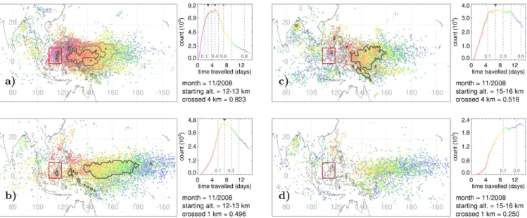
The first two questions we posed in Sect. 1 related to the time-scales, and the preferential locations, for transport from the boundary layer to the TTL. To begin to address these questions for our region of interest, the maps in Fig. 1 show where trajectories started above Borneo in November 2008 between 12–13 km, and 15–16 km, first cross 1 km and 4 km. To the right of each map is a probability distribution of the time it takes for trajectories to cross the altitude in question.

Figure 1a shows that back trajectories which started be-tween 12–13 km are most likely to cross 4 km after 3–5 days, and after∼6 days half of the trajectories have crossed 4 km. The most likely location for crossing 4 km is∼20◦_{E of the}

region where the trajectories start. The situation is similar when crossing altitudes of 5 km and 6 km are considered (not shown). So in this case study the modelled composition of the lower TTL above Borneo (between 12–13 km) is expected to be strongly influenced by the composition of the mid-troposphere (4–6 km)∼5 days beforehand; this timescale is significantly shorter than the local lifetime of a VSLS such as CHBr3.

Figure 1b shows that around half of the trajectories that started between 12–13 km crossed 1 km within 15 days and it is most likely that a trajectory will cross 1 km after∼7 days. The most likely crossing location is a narrow-latitude band further to the east, which suggests that emissions in the West-ern Pacific might be particularly important for the lowest part of the TTL over Borneo.

Figure 1c and d consider trajectories started between 15– 16 km, and contain many of the features found in plots a and b. A significant fraction of trajectories, more than half, cross 4 km within the 15 day calculation, and they are most likely to do so∼20–30◦E of their starting location. Approx-imately a quarter of trajectories starting in this altitude range cross 1 km; this is half as many as do so when started be-tween 12–13 km. The boundary layer in the Western Pacific region also appears to be an important source of air for the TTL at 15–16 km above Borneo.

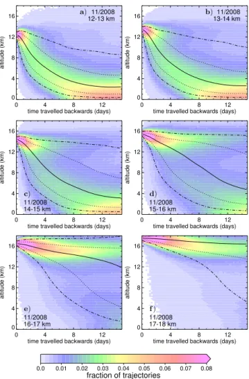
The previous analysis does not tell us about the details of transport between the boundary layer and the TTL, and does not account for those trajectories that do not reach either 1 km or 4 km within 15 days. More detail is given in Fig. 2 which shows, for trajectories starting in 1 km intervals between 12– 18 km in November 2008, the probability that a trajectory is at a particular altitude as it travels backwards in time.

(4)

Fig. 1.The maps show trajectory crossing locations. Back trajectories start at random within the red rectangle throughout November 2008. In(a)and(b)trajectories start between 12–13 km, in(c)and(d)trajectories start between 15–16 km. The coloured dots in(a)and(c)show where a random sample of 5 % of trajectories first crossed 4 km above the surface, while(b) and(d)show the same for 1 km. The dots are coloured by the time taken to cross either 1 or 4 km. To the right of each map are probability distributions of crossing times (6 h bins), where the colour of the line relates to the colours of the dots in the map. Successive deciles are marked with dashed grey lines, and the total fraction of trajectories that cross within 15 days is noted below. Where there are sufficient trajectories, the grey down-turned triangles mark the fraction crossing within the contour of the same colour on the map.

only∼5.5 days for 10 % of trajectories to cross 1 km. The difference is due to multiple crossings of 1 km by some tra-jectories. Following the 10th percentile lines in Fig. 2 (par-ticularly Fig. 2a–d, representing trajectories started between 12–16 km) also shows that transport from the boundary layer to∼4 km can take as long as transport between 4 km and the TTL. So, to reiterate, these trajectories suggest that mea-surements made in the TTL might bear a significantly clearer signature of air previously measured at∼4 km than of air pre-viously measured at∼1 km.

In Fig. 2 there are two dominant trajectory origins. In Fig. 2a (starting altitude 12–13 km) the majority of trajecto-ries originate in the lower troposphere, and in Fig. 2f (starting altitude 17–18 km) the majority of trajectories travel approx-imately horizontally within the upper TTL. An interesting in-termediate case is Fig. 2d (starting altitude 15–16 km) where a transition between these two regimes occurs.

The first population of trajectories, originating in the lower troposphere, are typically transported from the Western Pa-cific region (see Fig. 1). The second population of trajecto-ries, originating in the TTL, are typically transported from above the Asian subcontinent and follow an anti-cyclonic path to arrive above Borneo from the northeast (not shown). The trajectories presented in Figs. 1 and 2 therefore show that the TTL above Borneo is likely to be composed of two distinct types of air mass. They also suggest that it might not be possible to link measurements made at the surface in Borneo to measurements made in the TTL directly overhead.

Of course local individual convective events, which will also undoubtedly contribute to the TTL above Borneo to some de-gree, are not explicitly represented within our calculations.

2.2 Interannual variability

The third question we posed in Sect. 1 relates to the sensitiv-ity of transport to the year studied. We now consider interan-nual differences by comparing the calculations for November 2008 with similar calculations for the Novembers of 2006 (an El Ni˜no NH winter) and 2007 (La Ni˜na). By examining only three years we can not assess the entire range of year-to-year variability, but we can begin to characterise the different atmospheric conditions that hypothetical measurement cam-paigns in each of these years might encounter.

(5)

11/2008 12-13 km

0 4 8 12

time travelled backwards (days) 0

4 8 12 16

altitude (km)

a) 11/2008

13-14 km

0 4 8 12

4 8 12 16

altitude (km)

b)

11/2008 14-15 km

0 4 8 12

4 8 12 16

altitude (km)

c)

11/2008 15-16 km

0 4 8 12

4 8 12 16

altitude (km)

d)

11/2008 16-17 km

0 4 8 12

4 8 12 16

altitude (km)

e₎

11/2008 17-18 km

0 4 8 12

4 8 12 16

altitude (km)

f₎

0.0 0.01 0.02 0.03 0.04 0.05 0.06 0.07 0.08

fraction of trajectories

Fig. 2.Probability distributions of trajectory altitude as a function

of time travelled backwards during November 2008. Plot(a)shows trajectories started between 12–13 km, and(b–f)are for successive 1 km increases in starting altitude. Trajectories are grouped in to bins of 0.25 km (total 72) and 0.25 days (total 60). The median tra-jectory altitude is marked with a solid black line; 25th and 75th percentiles are marked with dotted lines; 10th and 90th percentiles are marked with dot-dash lines.

than in 2008 up to∼13.5 km, but larger above∼13.5 km; the trends are similar when 4 km is considered.

Further details of the differences between the years are shown in Fig. 4, which compares 1 km crossing locations for trajectories started between 12–13 km in each November. As in 2008, during the 2006 El Ni˜no, the Western Pacific is the most likely location for trajectories to cross 1 km. How-ever, less than half as many trajectories reach 1 km in 2006 as do so in 2008 (see also Fig. 3). The pattern during the 2007 La Ni˜na is slightly different. While the Western Pacific remains important, trajectories are also likely to cross 1 km in an arc stretching westwards to the island of Sumatra. The fraction of trajectories started between 12–13 km that cross

11/2006

11/2007

11/2008

Z = 1 km Z = 4 km

0.0 0.2 0.4 0.6 0.8 1.0 fraction crossing Z km in 15 days 0

4 8 12 16

start altitude / km

Fig. 3.For each of the three Novembers studied, the fraction of back

trajectories starting in 1 km bins between 7–18 km that cross 1 km (solid lines) and 4 km (dot-dash lines) within 15 days.

1 km during 2007 is approximately equal to the fraction in 2008 (again shown in Fig. 3).

Figure 5 considers trajectories started between 15–16 km. In all three years the Western Pacific is the dominant bound-ary layer source to this altitude range in the TTL over Bor-neo. However, the fraction of trajectories that reach 1 km is quite different in each year, with more than 3 times as many doing so in 2007 than in 2006. Another metric for year-to-year variability is the time taken for 10 % of trajectories started between 15–16 km to reach 1 km:∼13 days in 2006,

∼6 days in 2007 and∼9 days in 2008. VSLS measurements made in the TTL, in a particular year, need to be interpreted with this type of variability in mind.

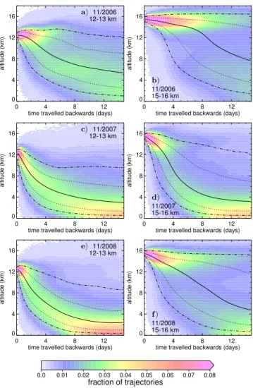
Interannual differences are also apparent in Fig. 6, which compares the 12–13 km and 15–16 km altitude versus time probability distributions for November 2008 (Fig. 2a and d) with the Novembers of 2006 and 2007. In the case of trajecto-ries started between 12–13 km, the 2006 El Ni˜no is again an outlying year, with the rate at which the trajectories ascend towards the TTL far slower than in the other years. At this starting altitude 2007 and 2008 are similar, though the pop-ulation of trajectories that originate in the lower troposphere are more densely packed in the ENSO-neutral 2008 than in the La Ni˜na of 2007. The behaviour of the trajectories started between 15–16 km is different in each of the years studied. In 2006, most of the trajectories travel at a fairly constant al-titude towards the TTL above Borneo, while in 2007, most originate in the lower troposphere. And in 2008, as noted in Sect. 2.1, there is an approximately even split between these two distinct source altitudes.

2.3 Variability of an idealised VSLS in the TTL

(6)

a) ₈₀ ₁₀₀ ₁₂₀ ₁₄₀ ₁₆₀ ₁₈₀ _-160

0 20

0 4 8 12 0.0

507.4 1014.8 1522.1 2029.5

0 4 8 12 time travelled (days) 0.0 0.5 1.0 1.5 2.0 count (10 3) 0.1 0.2

month = 11/2006 starting alt. = 12-13 km crossed 1 km = 0.216

b) ₈₀ ₁₀₀ ₁₂₀ ₁₄₀ ₁₆₀ ₁₈₀ _-160

0 20

0 4 8 12 0.0

858.8 1717.7 2576.5 3435.3

0 4 8 12 time travelled (days) 0.0 0.9 1.7 2.6 3.4 count (10 3)

0.1 0.2 0.3 0.4

c) ₈₀ ₁₀₀ ₁₂₀ ₁₄₀ ₁₆₀ ₁₈₀ _-160

0 20

0 4 8 12 0.0

1190.2 2380.4 3570.6 4760.8

Fig. 4.As for Fig. 1 but focussing on trajectories started between

12–13 km for the Novembers of 2006, 2007 and 2008.

as CHBr3, in the TTL. The method we use to answer this

question is simple; how sensitive our results might be to the assumptions we make is addressed later, in Sect. 4. Our cal-culations use an idealised tracer with an e-folding lifetime of 15 days (henceforth T15), which is comparable to that expected for CHBr3in the tropics. Exponential loss is likely

to be a reasonable approximation for a species such as CHBr3

that is lost primarily by photolysis.

The method first follows a trajectory, started in the TTL, backwards in time until it reaches 1 km above the surface; this altitude is used as a proxy for an encounter with a well-mixed boundary layer. The same trajectory is then followed forwards, from 1 km to its destination in the TTL, and the tracer, T15, is depleted exponentially along its path. We av-erage over all trajectories of interest (e.g. those started from a particular altitude, or started at a certain time) and assume that those trajectories not reaching the boundary layer within 15 days contribute zero, and act to dilute the tracer concentra-tion in the TTL. The term “T15 fracconcentra-tion” is used to describe the fraction of T15 that reaches the TTL relative to an initial-isation of unity at 1 km.

We wish to consider the variability in T15 fraction over the course of the months we have considered, and to do this have split each month in to 120 periods of 6 h. Figure 7 shows, for TTL altitude ranges of 12–13 km and 15–16 km, the temporal evolution of T15 fraction over each November considered, and summarises the temporal variability within each month. At each altitude range, and over each November,

a) 80 100 120 140 160 180 -160

0 20

0 4 8 12 0.0

420.2 840.4 1260.6 1680.8

0 4 8 12 time travelled (days) 0.0 0.4 0.8 1.3 1.7 count (10 3) 0.1

b) ₈₀ ₁₀₀ ₁₂₀ ₁₄₀ ₁₆₀ ₁₈₀ _-160

0 20

0 4 8 12 0.0

978.7 1957.5 2936.2 3914.9

0 4 8 12 time travelled (days) 0.0 1.0 2.0 2.9 3.9 count (10 3)

0.1 0.3 0.4

c) ₈₀ ₁₀₀ ₁₂₀ ₁₄₀ ₁₆₀ ₁₈₀ _-160

0 20

0 4 8 12 0.0

610.5 1221.0 1831.5 2442.0

Fig. 5.As for Fig. 1 but focussing on trajectories started between

15–16 km for the Novembers of 2006, 2007 and 2008.

there is significant variability; the implication here is that sampling the TTL on two different days might lead to very different measured distributions. The same applies to mea-surements made at different altitudes. For example, Fig. 7 shows that statistically similar T15 fractions are calculated for 12–13 km during the Novembers of 2007 and 2008. But, the pattern is different at 15–16 km, where the T15 fraction during the 2007 La Ni˜na is, on average, almost twice that during November 2008.

3 Existing aircraft measurements

As we note in Sect. 2, to date there have been no measure-ments of VSLS in the TTL over Southeast Asia. However, some observations, made in other parts of the tropics, do ex-ist. In this section, we describe data collected in the TTL over Central America, and then in Sect. 4 we present further tra-jectory calculations that can be compared directly with these measurements in an attempt to justify our methodology.

Two examples of aircraft campaigns that have measured VSLS in the TTL are the NASA campaigns CR-AVE and TC4, which were both based in Costa Rica, and sampled the TTL largely over the eastern Pacific adjacent to central America. CR-AVE took place during January and February 2006. Local TTL vertical transport rates have been inferred from CR-AVE measurements of CO2 and other species by

(7)

11/2006 12-13 km

0 4 8 12

4 8 12 16

altitude (km)

a)

11/2006 15-16 km

0 4 8 12

4 8 12 16

altitude (km)

b₎

11/2007 12-13 km

0 4 8 12

4 8 12 16

altitude (km)

c)

11/2007 15-16 km

0 4 8 12

4 8 12 16

altitude (km)

d)

11/2008 12-13 km

0 4 8 12

4 8 12 16

altitude (km)

e₎

11/2008 15-16 km

0 4 8 12

4 8 12 16

altitude (km)

f₎

0.0 0.01 0.02 0.03 0.04 0.05 0.06 0.07 0.08

fraction of trajectories

Fig. 6.Probability distributions of trajectory altitude as a function

of time travelled backwards during November 2006(a, b), 2007(c, d)and 2008(e, f). Plots(a),(c)and(e)show trajectories started be-tween 12–13 km, and plots(b),(d)and(f)show trajectories started between 15–16 km. See additional information in Fig. 2.

as far away as the Western Pacific influenced the observed chemical composition. In the following analysis we have considered CR-AVE measurements made by whole air sam-pler (WAS) on the 10 WB-57 flights that collected more than 10 samples between 11–17.5 km within the tropics. The WAS comprised 50 1.5-l electropolished stainless steel canis-ters equipped with automated metal valves which were pres-surised to 40 psi using a 4-stage bellows pump in flight (Flocke et al., 1999).

The TC4 campaign (Toon et al., 2010) occurred in July and August 2007 and featured 3 NASA aircraft. A summary of the aims of each days flights is provided by Toon et al. (2010) but a key point is that many TTL samples were collected in the vicinity of deep convection. Pfister et al. (2010) provide a meteorological overview of the campaign and note that the beginnings of a La Ni˜na led to lower than average levels of deep convection. Again making use of CO2measurements,

a)

01/11 06/11 11/11 16/11 21/11 26/11 0.0

0.2 0.4 0.6 0.8

fraction of T15 at 12-13 km

12-13 km

count

b)

01/11 06/11 11/11 16/11 21/11 26/11 Date

0.0 0.2 0.4 0.6 0.8

fraction of T15 at 15-16 km

060708

15-16 km

count

Fig. 7. Plot (a) shows a timeseries of the fraction of T15 (a

CHBr3 like tracer) relative to an initialisation value at 1 km that

reaches an altitude of 12–13 km above Borneo for the Novembers of 2006–2008. A statistical summary is provided by (1) the “box and whisker” plot to the right, with the monthly mean marked with a square, the bold lines denoting±1 standard deviation, and the dot-ted line representing the range and (2) a probability distribution to the far right (bin size 0.05). Plot(b)provides the same information, but for an altitude of 15–16 km.

Park et al. (2010) found that upward motion in the TTL was slower during TC4 than it had been during CR-AVE. In the following sections, we examine TTL data from the 3 tropical WB-57 flights.

We focus on observations of 3 VSLS with predominantly natural, oceanic sources: CH2Br2, CHBr3 and methyl

io-dide (CH3I). The 3 compounds have, under particular

ox-idative conditions, lifetimes of 123, 24 and 7 days respec-tively (Montzka and Reimann, 2011). These lifetimes are of course variable; for example, models suggest that CHBr3has

a shorter,∼15 day lifetime in the tropical troposphere and CH2Br2a longer, 6–12 month lifetime in the TTL (e.g.

War-wick et al., 2006; Liang et al., 2010; Hossaini et al., 2010; Park et al., 2010). Nevertheless, this range of lifetimes means that these compounds are expected to have varying strato-spheric impacts (see Gettelman et al., 2009; Aschmann et al., 2009).

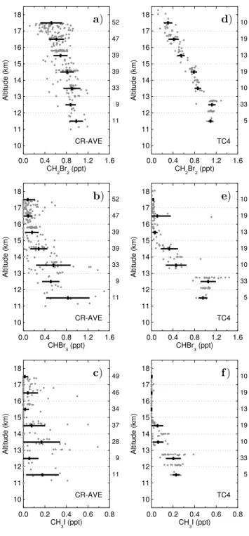
Data collected during both CR-AVE and TC4 are pre-sented in Fig. 8. There are clear differences between the cam-paigns. During CR-AVE the rate at which the abundance of each species decreases with altitude is relatively slow (see Park et al., 2010), and there is significant variability through-out the TTL. For example, at∼17 km CH2Br2ranges over

an order of magnitude and CHBr3 between∼0–0.5 ppt. In

contrast, during TC4 the negative gradients are steeper, there is less variability in the observations within each altitude bin, and very low concentrations of CHBr3and CH3I were found

(8)

0.0 0.4 0.8 1.2 1.6 CH

2Br2 (ppt) 10 11 12 13 14 15 16 17 18 Altitude (km) CR-AVE 11 9 33 39 39 47 52 a₎

0.0 0.4 0.8 1.2 1.6 CH

2Br2 (ppt) 10 11 12 13 14 15 16 17 18 Altitude (km) TC4 5 33 10 19 13 19 10 d₎

0.0 0.4 0.8 1.2 1.6 CHBr

3 (ppt) 10 11 12 13 14 15 16 17 18 Altitude (km) CR-AVE 11 9 33 39 39 47 52 b₎

0.0 0.4 0.8 1.2 1.6 CHBr

3 (ppt) 10 11 12 13 14 15 16 17 18 Altitude (km) TC4 5 33 10 19 13 19 10 e₎

0.0 0.2 0.4 0.6 0.8 CH

3I (ppt) 10 11 12 13 14 15 16 17 18 Altitude (km) CR-AVE 11 9 28 37 34 46 49 c₎

0.0 0.2 0.4 0.6 0.8 CH

3I (ppt) 10 11 12 13 14 15 16 17 18 Altitude (km) TC4 5 33 10 19 13 19 10 f₎

Fig. 8.Selected halocarbons measured by whole air sampler aboard

the WB-57 during CR-AVE(a–c)and TC4(d–f). Plots(a)and(d)

show CH₂Br₂,(b)and(e)show CHBr₃, and(c)and(f)show CH₃I; so lifetimes decrease from top to bottom. The number of measure-ments in successive 1 km altitude bins is noted to the right of each plot. The solid black lines show the mean±1 standard deviation in each bin.

In the following section we perform further trajectory cal-culations that aim to test the methodology with which, in Sect. 2, we reached conclusions concerning the time and lo-cation of transport pathways to the TTL over Borneo. Can

our method qualitatively reproduce the behaviour observed during CR-AVE and TC4?

4 Trajectory study related to aircraft measurements

In our second set of calculations we release batches of 10 000 15-day back trajectories from the time and location of each individual measurement in Fig. 8 (230 measurements in CR-AVE, 112 in TC4, which gives a total of 3.42 million trajec-tories). As in Sect. 2.3, we calculate the fraction of an ex-ponentially depleted tracer initialised at 1 km that remains at its destination in the TTL. Here, we use two lifetimes: 15 days, which can be compared to CHBr3observations, and

5 days, for comparison with CH3I. Accordingly, we refer to

the tracer remaining in the TTL as “T15 fraction” or “T5 fraction”.

Figure 9 shows, for both campaigns, the tracer fraction for batches of trajectories released for each of the samples. If ini-tially only the shapes of the tracer fraction profiles are con-sidered, then the observed differences between the 2 cam-paigns (Fig. 8) are reproduced: (1) the negative gradient is shallower during CR-AVE than during TC4; (2) tracer frac-tions within each altitude bin during CR-AVE are more vari-able than those during TC4; (3) there is a clear discontinuity in the TC4 tracer fractions at ∼15 km, above which near-zero tracer fractions are calculated. Tracer fractions are, in general, underestimated above∼15 km in CR-AVE, and be-tween∼11–13 km in TC4. Another way to look at these data is presented in Fig. 10, where for both campaigns, the CHBr3

observations are compared directly with calculated T15 frac-tions. Agreement between model and observation is closest where data lie near the grey lines. Again, it is clear that our trajectory calculations lead to too small a T15 fraction in the upper TTL during CR-AVE. We suggest one possible reason for this in Sect. 5.

Figures 8, 9 and 10 show that the trajectory calculations, as campaign means, are in many respects consistent with the observations. However, they do not provide any informa-tion about the ability of the trajectories to reproduce the ob-served day-to-day variability. In Fig. 11 we compare CHBr3

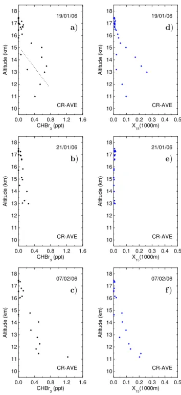
observations from individual flights with the calculated T15 fraction. We have selected 3 of the 10 CR-AVE flights for this analysis; the 19 and 21 January, and the 7 February. On each of these days measurements were made through most of the depth of the TTL. In addition, relatively low concen-trations of CH3I were observed on these days, so we

ex-pect that the measured air masses had not been heavily influ-enced by oceanic convection in the past few days. On each of these days we find that the shape of the calculated T15 fraction profile compares well with the CHBr3observations.

On 19 January the latitudinal difference (see the caption of Fig. 11) is clearly reproduced qualitatively in the calculated T15 fraction. On 21 January relatively low CHBr3

(9)

0.0 0.1 0.2 0.3 0.4 0.5 X₁₅(1000m) 10

11 12 13 14 15 16 17 18

Altitude (km)

CR-AVE a₎

0.00 0.05 0.10 0.15 0.20 X₀₅(1000m) 10

11 12 13 14 15 16 17 18

Altitude (km)

CR-AVE b₎

0.0 0.1 0.2 0.3 0.4 0.5 X

15(1000m) 10

11 12 13 14 15 16 17 18

Altitude (km)

TC4 c₎

0.00 0.05 0.10 0.15 0.20 X

05(1000m) 10

11 12 13 14 15 16 17 18

Altitude (km)

TC4 d₎

Fig. 9.TTL tracer fraction (i.e. assuming a boundary layer

concen-tration of 1) calculated from NAME back trajectories

correspond-ing to the measurements presented in Fig. 8 for CR-AVE(a, b)

and TC4(c, d). The tracer is initialised at 1 km a.g.l. In(a)and

(c)the tracer has an e-folding lifetime of 15 days, in(b) and(d)

an e-folding lifetime of 5 days. The solid dark blue lines show the mean_±1 standard deviation in each 1 km altitude bin. Note that the horizontal scales are not all the same.

calculated T15 fractions are consistent with the observations. And finally, on 7 February, CHBr3was observed to decrease

with altitude at a fairly uniform rate. Once more, the T15 fraction profile is similar.

To scale both the T5 and T15 fractions to the CH3I and

CHBr3measurements requires a factor of, in both cases,∼4

(see the grey lines in Fig. 10 for T15). The calculations are therefore consistent with boundary layer concentrations of 4 ppt of both species. Such mixing ratios have generally been observed only where sources are nearby, and are double what might be regarded as “background” levels (e.g. CHBr3

mea-surements reported by Yokouchi et al., 2005; Carpenter et al., 2005; Zhou et al., 2008; Pyle et al., 2011).

Given the simplicity of our approach, we consider the agreement to be reasonably good. Nevertheless, we now con-sider three possible sources of uncertainty (trajectory length, tracer lifetime and altitude of initialisation) in order to get an

a)

10-2

10-1

100

observed CHBr₃ (ppt) 10-3

10-2 10-1

NAME X

15

(1000m)

1 2 4

10

CR-AVE r2 = 0.37

b)

10-2

10-1

100

observed CHBr₃ (ppt) 10-3

10-2

10-1

NAME X

15

(1000m)

1 2 4

10

TC4 r2 = 0.48

altitude (km)1112131415161718

Fig. 10.The correlation between observed CHBr₃ and modelled

T15 during CR-AVE (plot(a), data from Fig. 8b and Fig. 9a) and TC4 (plot(b), data from Fig. 8e and Fig. 9c). The dots are coloured by altitude – see the legend at the bottom of plot(b). The grey lines indicate where there is a linear relationship between observation and model, and the scaling factor required to match model to observa-tion is noted at the left end of each line. Note that CHBr3was not

detected in 47 (2) out of 230 (112) samples collected during CR-AVE (TC4); these data are not presented in plot(a)or(b), though they are included in the correlation coefficient calculations.

idea of their possible importance. We recognise that this is an incomplete analysis, not least because of the problems in assessing the quality of the wind fields.

If we extend a subset of the trajectory calculation to 30 days then, typically, less than∼10 % (∼3 %) of T15 is un-accounted for in the lower (upper) TTL by considering only the first 15 days of travel. So, while a relatively small deficit, this simplification clearly contributes to the model underes-timation of the CHBr3observations. This is particularly true

(10)

0.0 0.4 0.8 1.2 1.6 CHBr

3 (ppt) 10

11 12 13 14 15 16 17 18

Altitude (km)

CR-AVE 19/01/06

a₎

0.0 0.1 0.2 0.3 0.4 0.5 X

15(1000m) 10

11 12 13 14 15 16 17 18

Altitude (km)

CR-AVE 19/01/06

d₎

0.0 0.4 0.8 1.2 1.6 CHBr

3 (ppt) 10

11 12 13 14 15 16 17 18

Altitude (km)

CR-AVE 21/01/06

b₎

0.0 0.1 0.2 0.3 0.4 0.5 X

15(1000m) 10

11 12 13 14 15 16 17 18

Altitude (km)

CR-AVE 21/01/06

e₎

0.0 0.4 0.8 1.2 1.6 CHBr

3 (ppt) 10

11 12 13 14 15 16 17 18

Altitude (km)

CR-AVE 07/02/06

c₎

0.0 0.1 0.2 0.3 0.4 0.5 X

15(1000m) 10

11 12 13 14 15 16 17 18

Altitude (km)

CR-AVE 07/02/06

f₎

Fig. 11.A comparison between CHBr₃observed on selected days

of CR-AVE(a–c)and NAME calculated profiles of a tracer with

15 day e-folding lifetime for the same sample locations and times

(d–f). The dashed line in(a)separates observations collected on two

different descents through the TTL; lower mixing ratios were found at∼10◦N, and higher mixing ratios found near the equator.

and a∼3 % increase in T15 would somewhat improve the linear fits presented in Fig. 10. There is a negligible (<1 %)

increase in T5 fraction when calculated with 30 day, rather than 15 day back trajectories. The assumption of a 15 day

lifetime for CHBr3is likely to be a valid approximation for

the atmosphere in which the trajectories travel (i.e. the trop-ical troposphere). As noted in Sect. 3, there is evidence for a marginally longer CHBr3 lifetime in the TTL; this is

an-other possible reason our calculations require high boundary layer concentrations to be consistent with the observations. If we adjust the initialisation altitude (recall this is a proxy for the assumed depth of a well-mixed boundary layer) to 1.5 km (0.5 km) then over the 15 day travel time∼15 % more (fewer) trajectories cross 1 km; these differences are relatively minor in our simplistic method.

We have also examined where the CR-AVE and TC4 back trajectories reach 1 km above the surface. Through their anal-ysis of CR-AVE measurements, Park et al. (2007) identified air masses likely to have originated locally, likely to have come from the Amazon, and likely to have travelled from the tropical Pacific. In Fig. 12a and b, which are analogous to Figs. 1, 4 and 5, we show that our trajectories are broadly consistent with Park et al. (2007). A small number of trajec-tories starting between 12–13 km reached the boundary layer locally within a few days. The tropical Atlantic is also an im-portant source, and a large fraction of our trajectories have travelled for 8–10 days from the tropical Western and Cen-tral Pacific boundary layer. However, few of our trajectories reach the boundary layer over the Amazon. Overall,∼25 % of CR-AVE trajectories starting between 12–13 km crossed 1 km within 15 days. Almost no trajectories started between 15–16 km reached the boundary layer locally, or over the At-lantic. Instead, the South Pacific convergence zone appears to be the most important boundary layer source for air masses ending up in this altitude range, consistent with large-scale convection in this region.

Unlike CR-AVE, few TC4 trajectories reach the bound-ary layer over the Pacific, which is consistent with the strong prevailing easterly winds in TTL described by Pfister et al. (2010). Instead, most trajectories that reached 1 km did so over the Amazon, over the tropical Atlantic, and over West-ern Africa. There are some similarities between these results and the trajectory calculations of Pfister et al. (2010), though the methods used are quite different.

Fewer trajectories reach 1 km within 15 days during CR-AVE and TC4 than do so from the TTL above Borneo. At 12– 13 km, the Central America fractions are comparable with the 2006 Borneo fractions (during an El Ni˜no), but only half as large as the 2007 and 2008 Borneo fractions (respectively, La Ni˜na and ENSO-neutral NH winters). At 15–16 km, the differences are more marked. For example,∼3 % of the TC4 trajectories reached 1 km, and 4 months later, in November 2007,∼42 % of trajectories started over Borneo did so.

5 Discussion and conclusions

(11)

Fig. 12.On the left of each plot, maps of trajectory 1 km crossing locations during CR-AVE(a, b)and TC4(c, d). 10000 back trajectories start at each sample location (dark red crosses) in the following altitude bands: in(a)and(c)trajectories start between 12–13 km, in(b)and

(d)between 15–16 km. Refer to Fig. 1 for additional information.

was to assist the planning of aircraft campaigns focussed on improving our knowledge of transport into and through the TTL. We have examined the conditions which might prevail for a future campaign and looked at 2 previous campaigns in order to test the validity of the approach. In the longer-term this approach should prove valuable in planning flights for long duration aircraft such as the unmanned Global Hawk where many more measurements can be made.

VSLS measurements have been made from high-flying air-craft during CR-AVE (January and February 2006) and TC4 (July and August 2007). Batches of back trajectories were run from a selection of these flights. The features of the ob-served vertical profiles of CHBr3and CH3I are broadly

sim-ilar to those of hypothetical tracers with 15 day and 5 day lifetimes. The drop-off with altitude was captured, as were differences between individual flights. As our method as-sumes a uniform VSLS concentration in the boundary layer, our results therefore suggest that the measurements exam-ined here were not affected by highly variable “hot spot” emissions. Consistent with previous work (Park et al., 2010), weaker uplift was found during TC4 than during CR-AVE. Nevertheless, our model calculations clearly underestimate the flux of VSLS to the upper TTL during CR-AVE; our interpretation is that NAME, and the underlying meteoro-logical analyses, accurately capture the main body of con-vective outflow between 11–14 km, but do not represent the stronger convective systems that reach higher altitudes. In terms of locations where air last left the boundary layer, there were marked differences between the two campaigns. Dur-ing CR-AVE the West Pacific was the main region of sup-ply, although the tropical Atlantic was also a contributor at lower altitudes (12–13 km). During TC4, however, boundary

layer air was predominantly sourced from the tropical At-lantic, South America and West Africa. These findings are broadly consistent with the dominant regions of convection in the two seasons.

The same approach has been used to aid campaign plan-ning for the SHIVA measurement phase during Novem-ber 2011. We used NovemNovem-ber 2008 (neutral) as our base case to investigate the origins of air in the TTL over Bor-neo. Our 2008 trajectories show that this particular part of the TTL consists of two regimes. Air in the lower TTL typically comes from the lower troposphere (below 4 km) with rapid upward transport occurring over several days prior to arriv-ing. Though of course we have used three-dimensional wind fields without an explicit representation of convection, this result appears to support the concept that upward transport from the boundary layer occurs in more than one step, with low-level convection feeding rapid transport to the lower TTL from ∼4 km (Hosking et al., 2010). Air in the upper TTL has largely travelled quasi-horizontally through the TTL over the past 15 days. In 2008, the transition between these two regimes occurs at∼15–16 km. Most of the trajectories that reached the boundary layer travelled from the Western Pacific,∼20–40◦E of Borneo, suggesting that measurements of VSLS in the TTL over Borneo might be strongly influ-enced by the lower tropospheric concentrations in this region. We note that our calculations for the CR-AVE campaign also highlight the Western Pacific region as the dominant bound-ary layer source to 15–16 km during NH winter; further near-surface measurements of VSLS in the Western Pacific might therefore be particularly valuable.

(12)

were found. During the El Niño, there was much less upward transport to this part of the TTL, and the influence of the boundary layer in the Maritime Continent is much smaller. In La Niña conditions, the amount of upward transport to 12–13 km is similar to the neutral case, though there was a greater influence of the boundary layer close to Borneo. Up-ward transport to higher altitudes in the TTL was stronger during the La Niña than during neutral conditions. It is worth emphasising that we have focussed on a small, but probably important, part of the TTL, and the influence of ENSO will be different in other parts of the tropics.

More chemical measurements (of short- and long-lived species) will be required to understand the transition between 12 km and the stratosphere. High altitude observations, such as those from the long duration Global Hawk, could play a valuable role in this. In order to maximise the information gathered from these flights, the approach presented here can be developed further to guide the aircraft into regions of spe-cific interest (e.g. where the influence of the boundary layer is weak, intermediate or strong). In conjunction with high-resolution mesoscale models capable of simulating convec-tion, it should also be possible to investigate the locations where local convection is important. This is challenging be-cause the variability is high (see Sect. 2.3), and statistical approaches based upon large numbers of measurements are likely to be needed to extract the required information.

Acknowledgements. This work was supported by the European

Commission through the SHIVA project (FP7-ENV-2007-1-226224). Matt Ashfold thanks NERC for a research studentship. Neil Harris is supported by a NERC Advanced Research Fellow-ship. We also thank Glenn Carver for help with running NAME.

Edited by: P. Haynes

References

Aschmann, J., Sinnhuber, B.-M., Atlas, E. L., and Schauffler, S. M.: Modeling the transport of very short-lived substances into the tropical upper troposphere and lower stratosphere, Atmos. Chem. Phys., 9, 9237–9247, doi:10.5194/acp-9-9237-2009, 2009. Butler, J. H., King, D. B., Lobert, J. M., Montzka, S. A.,

Yvon-Lewis, S. A., Hall, B. D., Warwick, N. J., Mondeel, D. J., Ay-din, M., and Elkins, J. W.: Oceanic distributions and emissions of short-lived halocarbons, Global Biogeochem. Cy., 21, GB1023, doi:10.1029/2006GB002732, 2007.

Carpenter, L. J., Wevill, D. J., O’Doherty, S., Spain, G., and Sim-monds, P. G.: Atmospheric bromoform at Mace Head, Ireland: seasonality and evidence for a peatland source, Atmos. Chem. Phys., 5, 2927–2934, doi:10.5194/acp-5-2927-2005, 2005. Davies, T., Cullen, M. J. P., Malcolm, A. J., Mawson, M. H.,

Stan-iforth, A., White, A. A., and Wood, N.: A new dynamical core for the Met Office’s global and regional modelling of the atmo-sphere, Q. J. Roy. Meteorol. Soc., 131, 1759–1782, 2005. Dorf, M., Butler, J. H., Butz, A., Camy-Peyret, C., Chipperfield,

M. P., Kritten, L., Montzka, S. A., Simmes, B., Weidner, F., and

Pfeilsticker, K.: Long-term observations of stratospheric bromine reveal slow down in growth, Geophys. Res. Lett., 33, L24803, doi:10.1029/2006GL027714, 2006.

FAO Fisheries and Aquaculture Department: The State of World Fisheries and Aquaculture 2010, Tech. rep., Food and Agricul-ture Organization of the United Nations, Rome, 2010.

Flocke, F., Herman, R. L., Salawitch, R. J., Atlas, E., Webster, C. R., Schauffler, S. M., Lueb, R. A., May, R. D., Moyer, E. J., Rosenlof, K. H., Scott, D. C., Blake, D. R., and Bui, T. P.: An examination of chemistry and transport processes in the tropical lower stratosphere using observations of long-lived and short-lived compounds obtained during STRAT and POLARIS, J. Geophys. Res., 104, 26625–26642, doi:10.1029/1999JD900504, 1999.

Fueglistaler, S., Wernli, H., and Peter, T.: Tropical

troposphere-to-stratosphere transport inferred from trajectory

cal-culations, J. Geophys. Res.-Atmos., 109, D03108,

doi:10.1029/2003JD004069, 2004.

Fueglistaler, S., Dessler, A. E., Dunkerton, T. J., Folkins, I., Fu, Q., and Mote, P. W.: Tropical Tropopause Layer, Rev. Geophys., 47, RG1004, doi:10.1029/2008RG000267, 2009.

Gettelman, A. and Forster, P. D. F.: A Climatology of the Tropi-cal Tropopause Layer, Journal of the MeteorologiTropi-cal Society of Japan, 80, 911–924, 2002.

Gettelman, A., Lauritzen, P. H., Park, M., and Kay, J. E.:

Processes regulating short-lived species in the tropical

tropopause layer, J. Geophys. Res.-Atmos., 114, D13303, doi:10.1029/2009JD011785, 2009.

Gostlow, B., Robinson, A. D., Harris, N. R. P., O’Brien, L. M., Oram, D. E., Mills, G. P., Newton, H. M., Yong, S. E., and A Pyle, J.:µDirac: an autonomous instrument for halocarbon

mea-surements, Atmos. Meas. Tech., 3, 507–521, doi:10.5194/amt-3-507-2010, 2010.

Heyes, W. J., Vaughan, G., Allen, G., Volz-Thomas, A., P¨atz, H.-W., and Busen, R.: Composition of the TTL over Darwin: local mixing or long-range transport?, Atmos. Chem. Phys., 9, 7725– 7736, doi:10.5194/acp-9-7725-2009, 2009.

Hosking, J. S., Russo, M. R., Braesicke, P., and Pyle, J. A.: Mod-elling deep convection and its impacts on the tropical tropopause layer, Atmos. Chem. Phys., 10, 11175–11188, doi:10.5194/acp-10-11175-2010, 2010.

Hossaini, R., Chipperfield, M. P., Monge-Sanz, B. M., Richards, N. A. D., Atlas, E., and Blake, D. R.: Bromoform and dibro-momethane in the tropics: a 3-D model study of chemistry and transport, Atmos. Chem. Phys., 10, 719–735, doi:10.5194/acp-10-719-2010, 2010.

Hoyle, C. R., Mar´ecal, V., Russo, M. R., Allen, G., Arteta, J., Chemel, C., Chipperfield, M. P., D’Amato, F., Dessens, O., Feng, W., Hamilton, J. F., Harris, N. R. P., Hosking, J. S., Lewis, A. C., Morgenstern, O., Peter, T., Pyle, J. A., Reddmann, T., Richards, N. A. D., Telford, P. J., Tian, W., Viciani, S., Volz-Thomas, A., Wild, O., Yang, X., and Zeng, G.: Representation of tropical deep convection in atmospheric models – Part 2: Tracer trans-port, Atmos. Chem. Phys., 11, 8103–8131, doi:10.5194/acp-11-8103-2011, 2011.

(13)

US, doi:10.1007/978-0-387-68854-1 62, 2007.

Kr¨uger, K., Tegtmeier, S., and Rex, M.: Long-term climatology of air mass transport through the Tropical Tropopause Layer (TTL) during NH winter, Atmos. Chem. Phys., 8, 813–823, doi:10.5194/acp-8-813-2008, 2008.

Kr¨uger, K., Tegtmeier, S., and Rex, M.: Variability of residence time in the Tropical Tropopause Layer during Northern Hemisphere winter, Atmos. Chem. Phys., 9, 6717–6725, doi:10.5194/acp-9-6717-2009, 2009.

Laube, J. C., Engel, A., B¨onisch, H., M¨obius, T., Worton, D. R., Sturges, W. T., Grunow, K., and Schmidt, U.: Contribution of very short-lived organic substances to stratospheric chlorine and bromine in the tropics – a case study, Atmos. Chem. Phys., 8, 7325–7334, doi:10.5194/acp-8-7325-2008, 2008.

Lawrence, M. G. and Rasch, P. J.: Tracer Transport in Deep Con-vective Updrafts: Plume Ensemble versus Bulk Formulations, J. Atmos. Sci., 62, 2880–2894, doi:10.1175/JAS3505.1, 2005. Levine, J. G., Braesicke, P., Harris, N. R. P., Savage, N. H., and Pyle,

J. A.: Pathways and timescales for troposphere-to-stratosphere transport via the tropical tropopause layer and their relevance for very short lived substances, J. Geophys. Res.-Atmos., 112, D04308, doi:10.1029/2005JD006940, 2007.

Levine, J. G., Braesicke, P., Harris, N. R. P., and Pyle, J. A.: Sea-sonal and inter-annual variations in troposphere-to-stratosphere transport from the tropical tropopause layer, Atmos. Chem. Phys., 8, 3689–3703, doi:10.5194/acp-8-3689-2008, 2008. Liang, Q., Stolarski, R. S., Kawa, S. R., Nielsen, J. E., Douglass, A.

R., Rodriguez, J. M., Blake, D. R., Atlas, E. L., and Ott, L. E.: Finding the missing stratospheric Bry: a global modeling study of CHBr3 and CH2Br2, Atmos. Chem. Phys., 10, 2269–2286,

doi:10.5194/acp-10-2269-2010, 2010.

Mata, T. M., Martins, A. A., and Caetano, N. S.: Microal-gae for biodiesel production and other applications: A re-view, Renewable and Sustainable Energy Reviews, 14, 217–232, doi:10.1016/j.rser.2009.07.020, 2010.

Montzka, S. A. and Reimann, S.: Ozone-Depleting Substances (ODSs) and Related Chemicals, vol. Scientific Assessment of Ozone Depletion: 2010, Global Ozone Research and Monitoring Project – Report No. 52, chap. 1, World Meteorological Organi-zation (WMO), Geneva, 2011.

Morrison, N. L. and Webster, H. N.: An Assessment of Turbulence Profiles in Rural and Urban Environments Using Local Mea-surements and Numerical Weather Prediction Results, Bound.-Lay. Meteorol., 115, 223–239, doi:10.1007/s10546-004-4422-8, 2005.

O’Brien, L. M., Harris, N. R. P., Robinson, A. D., Gostlow, B., War-wick, N., Yang, X., and Pyle, J. A.: Bromocarbons in the tropical marine boundary layer at the Cape Verde Observatory – mea-surements and modelling, Atmos. Chem. Phys., 9, 9083–9099, doi:10.5194/acp-9-9083-2009, 2009.

Park, S., Jim´enez, R., Daube, B. C., Pfister, L., Conway, T. J., Got-tlieb, E. W., Chow, V. Y., Curran, D. J., Matross, D. M., Bright, A., Atlas, E. L., Bui, T. P., Gao, R.-S., Twohy, C. H., and Wofsy, S. C.: The CO2tracer clock for the Tropical Tropopause Layer,

Atmos. Chem. Phys., 7, 3989–4000, doi:10.5194/acp-7-3989-2007, 2007.

Park, S., Atlas, E. L., Jim´enez, R., Daube, B. C., Gottlieb, E. W., Nan, J., Jones, D. B. A., Pfister, L., Conway, T. J., Bui, T. P., Gao, R.-S., and Wofsy, S. C.: Vertical transport rates and

con-centrations of OH and Cl radicals in the Tropical Tropopause Layer from observations of CO2and halocarbons: implications

for distributions of long- and short-lived chemical species, At-mos. Chem. Phys., 10, 6669–6684, doi:10.5194/acp-10-6669-2010, 2010.

Paul, C. and Pohnert, G.: Production and role of volatile halo-genated compounds from marine algae, Natural Product Reports, 28, 186–195, 2011.

Pfister, L., Selkirk, H. B., Starr, D. O., Rosenlof, K., and Newman, P. A.: A meteorological overview of the TC4 mission, J. Geo-phys. Res., 115, D00J12, doi:10.1029/2009JD013316, 2010. Pisso, I., Haynes, P. H., and Law, K. S.: Emission

loca-tion dependent ozone depleloca-tion potentials for very short-lived halogenated species, Atmos. Chem. Phys., 10, 12025–12036, doi:10.5194/acp-10-12025-2010, 2010.

Pyle, J. A., Ashfold, M. J., Harris, N. R. P., Robinson, A. D., War-wick, N. J., Carver, G. D., Gostlow, B., O’Brien, L. M., Manning, A. J., Phang, S. M., Yong, S. E., Leong, K. P., Ung, E. H., and Ong, S.: Bromoform in the tropical boundary layer of the Mar-itime Continent during OP3, Atmos. Chem. Phys., 11, 529–542, doi:10.5194/acp-11-529-2011, 2011.

Quack, B. and Wallace, D. W. R.: Air-sea flux of bromoform: Con-trols, rates, and implications, Global Biogeochem. Cy., 17, 1023, doi:10.1029/2002GB001890, 2003.

Salawitch, R. J., Weisenstein, D. K., Kovalenko, L. J., Sioris, C. E., Wennberg, P. O., Chance, K., Ko, M. K. W., and McLinden, C. A.: Sensitivity of ozone to bromine in the lower stratosphere, Geophys. Res. Lett., 32, L05811, doi:10.1029/2004GL021504, 2005.

Schauffler, S. M., Atlas, E. L., Blake, D. R., Flocke, F., Lueb, R. A., Lee-Taylor, J. M., Stroud, V., and Travnicek, W.: Distributions of brominated organic compounds in the troposphere and lower stratosphere, J. Geophys. Res.-Atmos., 104, 21513–21535, 1999. Schofield, R., Fueglistaler, S., Wohltmann, I., and Rex, M.: Sen-sitivity of stratospheric Bryto uncertainties in very short lived

substance emissions and atmospheric transport, Atmos. Chem. Phys., 11, 1379–1392, doi:10.5194/acp-11-1379-2011, 2011. Toon, O. B., Starr, D. O., Jensen, E. J., Newman, P. A., Platnick, S.,

Schoeberl, M. R., Wennberg, P. O., Wofsy, S. C., Kurylo, M. J., Maring, H., Jucks, K. W., Craig, M. S., Vasques, M. F., Pfister, L., Rosenlof, K. H., Selkirk, H. B., Colarco, P. R., Kawa, S. R., Mace, G. G., Minnis, P., and Pickering, K. E.: Planning, imple-mentation, and first results of the Tropical Composition, Cloud and Climate Coupling Experiment (TC4), J. Geophys. Res., 115, D00J04, doi:10.1029/2009JD013073, 2010.

Tost, H., Lawrence, M. G., Br¨uhl, C., J¨ockel, P., The GABRIEL Team, and The SCOUT-O3-DARWIN/ACTIVE Team: Uncer-tainties in atmospheric chemistry modelling due to convection parameterisations and subsequent scavenging, Atmos. Chem. Phys., 10, 1931–1951, doi:10.5194/acp-10-1931-2010, 2010. Warwick, N. J., Pyle, J. A., Carver, G. D., Yang, X., Savage,

N. H., O’Connor, F. M., and Cox, R. A.: Global modeling of biogenic bromocarbons, J. Geophys. Res.-Atmos., 111, D24305, doi:10.1029/2006JD007264, 2006.

(14)

D23309, doi:10.1029/2005JD006303, 2005.

Yung, Y. L., Pinto, J. P., Watson, R. T., and Sander, S. P.: Atmo-spheric Bromine And Ozone Perturbations In The Lower Strato-sphere, J. Atmos. Sci., 37, 339–353, 1980.