www.ocean-sci.net/7/203/2011/ doi:10.5194/os-7-203-2011
© Author(s) 2011. CC Attribution 3.0 License.
Ocean Science
The effect of tides on dense water formation in Arctic shelf seas
C. F. Postlethwaite1, M. A. Morales Maqueda1, V. le Fouest2,*, G. R. Tattersall1,**, J. Holt1, and A. J. Willmott1
1National Oceanography Centre, Joseph Proudman Building, 6 Brownlow Street, Liverpool, L3 5DA, UK 2The Scottish Association for Marine Science, Dunstaffnage Marine Laboratory, Oban, PA37 1QA, UK
*present address: Laboratoire d’Oc´eanographie de Villefranche, BP 8 CNRS & l’Universit´e Pierre et Marie Curie (Paris VI),
06238 Villefranche-sur-Mer Cedex, France
**present address: Swathe Services, 1 Winstone Beacon, Saltash, Cornwall, PL12 4RU, UK
Received: 5 August 2010 – Published in Ocean Sci. Discuss.: 9 September 2010 Revised: 17 February 2011 – Accepted: 8 March 2011 – Published: 24 March 2011
Abstract. Ocean tides are not explicitly included in many ocean general circulation models, which will therefore omit any interactions between tides and the cryosphere. We present model simulations of the wind and buoyancy driven circulation and tides of the Barents and Kara Seas, using a 25 km×25 km 3-D ocean circulation model coupled to a
dy-namic and thermodydy-namic sea ice model. The modeled tidal amplitudes are compared with tide gauge data and sea ice extent is compared with satellite data. Including tides in the model is found to have little impact on overall sea ice extent but is found to delay freeze up and hasten the onset of melting in tidally active coastal regions. The impact that including tides in the model has on the salt budget is investigated and found to be regionally dependent. The vertically integrated salt budget is dominated by lateral advection. This increases significantly when tides are included in the model in the Pe-chora Sea and around Svalbard where tides are strong. Tides increase the salt flux from sea ice by 50% in the Pechora and White Seas but have little impact elsewhere. This study suggests that the interaction between ocean tides and sea ice should not be neglected when modeling the Arctic.
1 Introduction
Tidal mixing is believed to play a significant role in maintain-ing abyssal stratification (Egbert and Ray, 2000; Munk and Wunsch, 1998) and in controlling the entire water column structure in continental shelf seas (e.g., Sharples et al., 2001; Rippeth, 2005). Thus, omitting tides from ocean general
cir-Correspondence to:C. F. Postlethwaite ([email protected])
culation models (OGCMs) presents a problem for many re-gions, including, as we shall see in the following, the Arctic Ocean and its shelf seas. Holloway and Proshutinsky (2007) have highlighted the problem of neglecting the effects of tidal mixing in regions of Atlantic inflow to the Arctic and the potential for underestimating ventilation of deep waters in these regions. Tidal mixing within the water column and at the base of the sea ice cover can increase the heat flow from deeper water masses towards the surface causing decreased freezing and increased melting of sea ice and possibly the formation of sensible heat polynyas (Morales-Maqueda et al., 2004; Willmott et al., 2007; Lenn et al., 2010). The tidal currents can additionally increase the stress and strain on the sea ice and cause leads to open periodically within the sea ice cover (Kowalik and Proshutinsky, 1994). The ar-eas of open water exposed by such deformation of the sea ice are prone to intense winter heat loss (10–100 times larger than over sea ice, Maykut, 1982) and may in turn start to freeze, releasing salt to the underlying water as brine is re-jected from the ice matrix. Although leads are not large (at most a few kilometers in width), their periodic tidal reoccur-rence could mean that the dense water formed from rejected brine in leads is significant. In this paper we consider the impact of tides on sea ice cover and ocean stratification in an Arctic shelf sea region (Barents and Kara Seas) as simulated in a high-resolution regional OGCM.
rejection, whereas, in summer, it enhances the absorption of shortwave radiation by the oceanic mixed layer (Maykut and Perovich, 1987; Eisen and Kottmeier, 2000). Process 3 is the mechanical redistribution of ice itself caused by the alterna-tion of convergence and divergence periods during the tidal cycle. A fourth process, not shown in the schematic, is tidal generation of residual currents and the associated ice drift.
In general, global climate models do not explicitly rep-resent tides and high frequency oscillations. The horizon-tal resolution of climate models, such as those that con-tributed to the IPCC AR4 (Randall et al., 2007) are still too coarse (∼110–220 km) for tides to be appropriately captured
in them. For example, a 200 m deep shelf sea at 75◦N has
a barotropic Rossby radius and M2 tidal wavelength of ap-proximately 315 km, requiring at least∼100 km resolution.
Besides, the typical frequency of atmosphere-ocean coupling of∼24 h in IPCC-type models precludes the correct forcing
of ocean tides. Muller et al. (2010) address this omission and find that explicitly including tides in the Max Planck In-stitute for Meteorology climate model (ECHAM5/MPI-OM) improves simulations of the climate in Western Europe.
Traditionally, OGCMs have also neglected tidal processes. In the past, the reason for this was simply that the rigid lid representation of the ocean surface used in most of these models did not allow tides to be included. At present, how-ever, most OGCMs include a free surface and so can, in principle, accommodate tidal processes. Although model and computer advancement means that horizontal and ver-tical resolution are increasing in OGCMs such that the ex-plicit inclusion of the barotropic tide is possible (Arbic et al., 2010; Thomas and S¨undermann, 2001), they require substan-tial computer resources to run. Thus, regional models that can regularly operate on finer resolutions and shorter time steps are an efficient way to study tidal processes in Arctic shelf seas.
Holloway and Proshutinsky (2007) give a comprehensive review of previous high latitude tidal modeling studies so this is not repeated here. They also discuss two approaches to modeling the influence of tides in the Arctic Ocean, namely explicitly resolving the tides in a high resolution, three-dimensional coupled ocean/ice model or parameterising their
feedback on the modeled sea ice cover as new ice can form in the freshly exposed areas of open water when atmospheric temperatures are cold enough. The forcing for these param-eterizations are the time averaged total energy dissipation and time averaged water-column divergence provided by the barotropic tidal model of Kowalik and Proshutinsky (1994). Using this method, they complete a 1948–2005 integration of the sea ice-ocean system over the whole Arctic Ocean.
Rather than parameterising tidal effects on ocean mixing and sea ice motion, we explore in this paper the alternative method of explicitly modeling the leading tidal constituents in a three-dimensional coupled ocean/ice model, resolving the propagation of coastal trapped waves associated with tidal incursion on-shelf but not resolving the tidal excursion (<7 km). To do this we restrict ourselves to a 5 yr regional model simulation of the Barents and Kara Seas (Fig. 2). These seas are some of the most important in the Arctic, with the Barents Sea dominating Arctic Ocean heat loss to the atmosphere (Serreze et al., 2007) and the Kara Sea re-ceiving∼55% of the river discharge into the Siberian Arctic
(Pavlov and Pfirman, 1995). Warm Atlantic water undergoes intense cooling in the southern ice-free sector of the Barents Sea producing dense waters that may contribute to deep wa-ter formation in the Arctic (Rudels et al., 1994; Schauer et al., 2002). To the north and east, brine rejection from sea ice and polynya activity also contribute to dense water for-mation (Midttun, 1985). Tides are strong in the Barents Sea (the strongest in the Arctic apart from in the Canadian Arctic Archipelago, Padman and Erofeeva, 2004) and they play a significant role in dense water formation in the Arctic affect-ing stratification, circulation and sea ice.
2 Model description
Fig. 2. (a)Polar stereographic projection of the Arctic showing the study region. Black dots indicate the location of tide gauges. (b)Bathymetry of the Barents and Kara Seas domain. The 400 m contour is taken to be the boundary of the continental shelf region. The grey line shows the edge of the model domain. Colors indicate subdomains used in this study (the Kara Sea is shaded yellow, the White Sea is red, the Pechora Sea is blue, the region around Svalbard is green and the rest of the Barents Sea is grey).
2007; Andreu-Burillo et al., 2007). The details of the model are well documented in Holt and James (2001). It suffices here to mention that the model uses a one equation variant of the Mellor and Yamada (1974) turbulence closure scheme to calculate vertical mixing, handles hydrostatic instabilities with an iterative convective adjustment method, and does not include explicit tracer horizontal diffusion (small amounts of numerical diffusion in the piecewise parabolic advection scheme used by the model guarantee tracer stability). Hor-izontal viscosity is held constant at 1.0×10⁴m2s−1.
POL-COMS has been coupled to the Los Alamos sea ice model (CICE v3.14, Hunke and Lipscomb, 2004). CICE is a multi-category dynamic-thermodynamic sea ice model that uses an elastic-viscous-plastic rheology. The simulations presented here use a single ice category to ease comparison with the previous tide/ice study of Holloway and Proshutinsky (2007). Ice/ocean heat fluxes are calculated using the standard mixed layer option in CICE, which has been adapted so that the ocean temperatures used in the calculations are the temper-atures of the surface box of the ocean model. All other sea ice parameters are those described as standard in Hunke and Lipscomb (2004). The sea ice dynamics interacts with the tides via changes to the ice/ocean stress due to the tidal cur-rents and residual circulation. The sea ice thermodynamics interacts with the tides via the ice/ocean heat fluxes. These are driven by the sea surface temperature which is affected by tidal mixing. The model does not include any representation of landfast ice.
The model domain has open boundaries to three sides, hence external forcing fields are required for both the ocean and ice models. These are discussed in Sect. 2.1 along with the surface forcing used. Both ocean and sea ice models are constructed on a grid defined using a Cartesian coordinate system (x, y) with the origin at the North Pole, the x-axis in the direction of 90◦E and a resolution of 25 km in both
di-rections. This is similar to the coordinate system described in Gjevik and Straume (1989) but has the geometric scale factors associated with moving from a sphere to a Cartesian plain as constants. The domain spans 0◦E–110◦E and from
64◦N–84◦N, with 109 grid points in the x direction and 141
in the y direction. The ocean model has 30 vertical depths de-fined using sigma levels, whereby the vertical spacing of the sigma levels are allowed to vary in the horizontal using the S-coordinate transform of Song and Haidvogel (1994), which allows higher resolution to be maintained near the surface in deep water. The time steps used are 10 s for the barotropic and 600 s for both the baroclinic and the ice model.
2.1 Surface and boundary forcing
Fig. 3. (a)Contour plot of the M2 tidal elevation amplitude in meters (color with black contours. Contours are spaced every 0.1 m between 0 and 1 m and spaced every 0.5 m from 1–3 m) and phase in degrees (white contours).(b)M2 tidal ellipses.
surface, and Hunke and Lipscomb, 2004 for the air-ice inter-face). A climatological annual cycle of precipitation for this area is created from the data of Serreze and Hurst (2000). Initial conditions for 1 September 2000 and lateral boundary conditions for the ocean component are derived from the US Navy Research Laboratory Naval Coastal Ocean Model (1/8◦
global NCOM with 40 vertical levels, Barron et al., 2006, 2007; Martin et al., 2004). Six hourly three-dimensional fields of temperature, salinity and ocean velocities for the same time period as the atmospheric forcing are linearly interpolated onto the model grid over a relaxation zone of width 100 km around the lateral boundaries as described in Holt and James (2001). Initial and six hourly boundary con-ditions for ice concentration and thickness are provided by the Polar Ice Prediction System (Preller and Posey, 1996; Woert et al., 2004) and interpolated onto the same relaxation zone. No restoring was applied to the domain interior. Sea surface elevations and velocities for tidal forcing at the open boundaries are sourced from the TPXO6.2 medium resolu-tion global inverse tide model from Oregon State University (Egbert and Erofeeva, 2002) and are applied every barotropic time step. Eight tidal constituents are used: Q1, O1, P1, K1, N2, M2, S2 and T2. Freshwater input from the two largest rivers in the domain (the Ob and the Yenisei) are also in-cluded in the model. Daily values for the stream flow are cre-ated by averaging daily mean values from 1954–1999 for the river Ob and from 1955–1999 for the river Yenisei (GRDC, 2003).
2.2 Model runs
Results are presented here from two model runs, namely, – Run 1 – POLCOMS/CICE without tides (control run) – Run 2 – POLCOMS/CICE with tides.
In both cases, the model is integrated for 5 yr repeating the atmospheric and oceanic forcing for the September 2000– August 2001 period. Results from the last year of integra-tion, when the sea ice cover is approaching a cyclostationary state, are analyzed here. By comparing the results from these two experiments we evaluate the impact of including tidal dynamics on the modeled ice distribution, ice formation and brine rejection.
3 Results
3.1 Description of the modeled tides
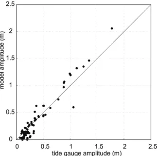
Fig. 4. Comparison of M2 model amplitude with tide gauge ob-servations (Gjevik and Straume, 1989; IHO, 1994; Kowalik and Proshutinsky, 1994, 1995).
Land (Fig. 3b). Figure 4 shows a comparison of the mod-eled M2 tidal amplitude with historical tide gauge data (Gje-vik and Straume, 1989; IHO, 1994; Kowalik and Proshutin-sky, 1994, 1995). The agreement between the simulated and gauged tidal amplitudes is quite reasonable (RMS devia-tion=12.1 cm, mean deviation=0.6 cm) although the phase
correspondence is not as good (RMS deviation=43◦, mean
deviation=6◦). The tide gauge observations are
predomi-nantly from coastal locations (Fig. 1) and no extrapolation or interpolation of the modeled data has been done in the com-parison; rather the model amplitude value at the grid point nearest to each tide gauge has been used. The simplicity of the approach along with the difficulty in modeling the prop-agation of coastal trapped waves around the complex coast-line is most likely responsible for the differences between the modeled and observed tides.
3.2 Impact of tides on sea ice distribution
Assessing the impact of tides on sea ice distribution is com-plicated by the sometimes opposing interactions between tides and ice, as tides can increase melting at the base of the sea ice through enhanced diapycnal mixing of warm deep water with surface cold water, but can also promote new ice production by opening new leads where freezing occurs. Prior to pursuing this assessment, we initially examine how well the model reproduces the location of the sea ice edge, which is defined as the line of 15% ice concentration. The location of the sea ice edge at the time of maximum ex-tent of the sea ice cover (March 2001) is comparable with remote sensing observations (Fig. 5). However, the sea ice
edge location at the time of minimum ice extent (Septem-ber) spreads somewhat southward of the observed one in the vicinity of Franz Josef Land (Fig. 5). Including tides in the model does not significantly improve the modeled ice ex-tent in this region and the September ice edge remains to the south of the observed edge. The modeled sea surface temperature remains several degrees Centigrade cooler than coincident observations in the northern part of the Barents Sea during the summer (Ingvaldsen et al., 2002). It is un-clear whether these discrepancies are a result of anomalous atmospheric forcing, to which sea ice is extremely sensitive (Hunke and Holland, 2007), or rather they reflect deficien-cies in the model, bulk formulae, boundary conditions or a biased state of the ocean and sea ice following the 5 yr spin up with repeat forcing from 2000–2001. In any case, these model errors do not unduly impact the present study into the interaction between tides and ice in our coupled ocean/sea ice model since the summer cold bias is present in both the control and tides simulations.
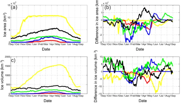
The net impact of including tides on the modeled sea ice distribution varies regionally. To investigate the spatial pat-terns of these changes the continental shelf region of the model domain has been divided into five subdomains defined by geographic and bathymetric boundaries. These subdo-mains are the White Sea, the Pechora Sea (shallower than 100 m), the Kara Sea (shallower than 400 m), the oceanic area around Svalbard (shallower than 200 m) and the rest of the Barents Sea (shallower than 400 m) (Fig. 2b). Time series of daily mean ice area and ice volume integrated over these five regions are plotted in Fig. 6a and c, respectively. The seasonal cycle of sea ice distribution in each subdomain dif-fers widely and is in good agreement with satellite observa-tions for all subdomains (Kern et al., 2010). The entire Kara Sea freezes rapidly during October and November and the ice continues to thicken until May. The Pechora and White Seas are ice free during the summer and freeze up occurs more gradually than in the Kara Sea. The area around Svalbard and the Barents Sea both retain ice in the summer months and have a gradual increase in sea ice during the winter.
The impact of including tides in the model on the sea ice area and volume varies between subdomains (Fig. 6b and d), and so also do the causes for these variations. Warmer sea surface temperatures, caused by enhanced vertical mixing, delays freeze up in the Pechora Sea when tides are included in the model, such that approximately 30% less of the sea surface is ice covered during December and January. With-out tides, haline stratification supports cooler water over-lying warmer water, whereas including tides in the model causes warmer water to get mixed to the surface earlier in the year. The same process speeds up melting in the White Sea, where there is 30% less ice cover during the melting sea-son when tides are included in the model. The actual changes in oceanic heat flux into the ice, however, are not very big, amounting to between 1 and 3 W m−2and causing a decrease
Fig. 5.Location of the ice edge when sea ice extent is at its’ maximum and minimum for(a)the control run,(b)the run including tides and (c)from remote sensing of brightness temperatures data (Cavalieri et al., 1996, updated 2008). The thin lines show the monthly mean ice edge for September 2000 and the heavy lines show the monthly mean ice edge for March 2001. The ice edge is defined as the line of 15% concentration.
Fig. 6. (a)Daily ice area integrated over the subdomains shown in Fig. 2b for the control model run.(b)Difference in ice area between the model run with and without tidal forcing integrated over each subdomain. Positive values indicate that the total ice area is greater with tidal forcing than without.(c)and(d)as above but for ice volume.
these oceanic heat flux anomalies are on the order of 10–20% of the net oceanic heat flux into the ice in the area. The area of open water within the sea ice (leads) increases by 50% in the Pechora Sea during March and April when tides are in-cluded in the model. Extra ice production ensues, resulting in a small increase in ice volume at this time (∼2.5 km3), with
ice becoming an average of 5 cm thicker. Advection of ice in from the northern and western boundaries of the domain increases when tides are included in the model and cause ice to pile up around Svalbard, leading to a 5–10% increase in ice volume (Fig. 6d).
Table 1. Net freezing integrated over the subdomains indicated in Fig. 2b for the model run with tides, the control run without tides and the differences between them (km3yr−1). Also shown in
brackets is the ice thickness increase brought about by this amount of net freezing when averaged over each subdomain (m yr−1).
Net Freezing With tides km3yr−1
(m yr−1)
Without tides km3yr−1
(m yr−1)
Difference km3yr−1
(m yr−1)
Pechora Sea 206 (0.80)
198 (0.77)
8 (0.03) Kara Sea 1154
(1.16)
1159 (1.17)
−5 (0.01) White Sea 39
(0.55) 39 (0.55) 0 (0.00) Svalbard 149 (0.55) 156 (0.57) −7 (−0.02) Barents Sea 384
(0.20) 381 (0.20) 3 (0.00) Deep 869 (0.68) 909 (0.72) −40 (−0.04)
than forms in situ. The deep region of the model domain that is not part of the continental shelf is dominated by melting but this area is heavily influenced by the boundary conditions and is not discussed further.
Including tides in the model increases net melting most significantly in the Svalbard region, where the tidal currents are strong. The impact on net freezing over the shelf varies from location to location with a small increase in freezing in the Pechora Sea and a small decrease around Svalbard. Al-though these differences correspond to relatively small vol-ume changes in sea ice, the shallow depths of some coastal regions means that, as we shall see below, the influence on local salinity and density can be large.
3.3 Impact of tides on salinity distribution
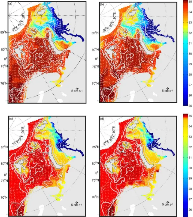
Residual currents, tidal mixing and changes to brine rejec-tion and sea ice melting all act to change the salinity dis-tribution of the water column when tides are added to a coupled ocean/sea ice model. As a first attempt at estab-lishing how tidal processes change the salinity distribution in the model, we compare the sea surface and sea bottom salinity (the salinity in the uppermost/lowermost model grid cells, respectively) between the two model runs for both win-ter and summer. Summer and winwin-ter mean sea surface and sea bottom salinity for the control model run are contoured in Fig. 7. The salty Norwegian Atlantic Current enters the domain at the southern open boundary. One branch, the North Cape Current, enters the Barents Sea following the Norwegian coastline. A second branch, the West
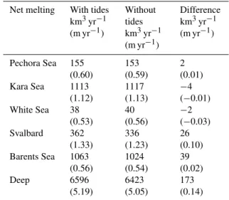
Spitsber-Table 2. Net melting integrated over the subdomains indicated in Fig. 2b for the model run with tides, the control run without tides and the differences between them (km3yr−1). Also shown in
brackets is the ice thickness decrease brought about by this amount of net melting when averaged over each subdomain (m yr−1).
Net melting With tides km3yr−1
(m yr−1)
Without tides km3yr−1
(m yr−1)
Difference km3yr−1
(m yr−1)
Pechora Sea 155 (0.60)
153 (0.59)
2 (0.01) Kara Sea 1113
(1.12)
1117 (1.13)
−4 (−0.01) White Sea 38
(0.53)
40 (0.56)
−2 (−0.03) Svalbard 362 (1.33) 336 (1.23) 26 (0.10) Barents Sea 1063
(0.56) 1024 (0.54) 39 (0.02) Deep 6596 (5.19) 6423 (5.05) 173 (0.14)
Fig. 7.Mean sea surface salinity (color contours) and velocity (arrows) for(a)winter and(b)summer from the fifth year of integration of the control model run (without tides). Mean sea bottom salinity (color contours) and velocity (arrows) for(c)winter and(d)summer from the fifth year of integration of the control model run (without tides). 50 m, 200 m 400 m and 1000 m bathymetric contours are shown. Winter is defined as December, January, February and summer is defined as June, July, and August. For clarity, the velocity vectors are capped at 5 cm s−1.
4 Discussion
We are interested in how tides affect dense water formation via brine rejection in the model. CICE does not include a formulation of salt release or entrapment upon ridging nor does the mixing scheme in POLCOMS account for addi-tional stirring caused by sea ice fracture and pile up. As
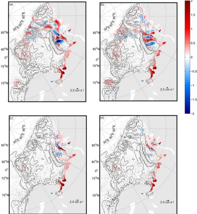
Fig. 8.Mean difference in sea surface salinity (color contours) and velocity (arrows) between the model run with tides and the control run for(a)winter and(b)summer from the fifth year of model integration. Mean difference in sea bottom salinity (color contours) and velocity (arrows) for(c)winter and(d)summer from the fifth year of model integration. Winter and summer as defined in Fig. 7. Positive values indicate the salinity is greater when tides are included in the model. The velocity vectors are capped at 2.5 cm s−1.
salinity as freshwater is released during melting. Moreover, changes to the amount of open water will affect the surface freshwater fluxes by altering both the amount of evapora-tion that can occur and how much precipitaevapora-tion enters the ocean (in the model, snow falling on ice does not enter the ocean until the snow melts or ridging occurs, whereas pre-cipitation falling directly into the ocean has an immediate effect on salinity). However, other processes affected by the tides may also act to change the salinity structure, for
exam-ple tidally enhanced vertical or horizontal mixing of different water masses or salt transport by residual tidal currents. Here we discuss which of the changes to the water column salt budget are directly attributable to tide/ice interactions rather than other tidally related processes.
4.1 Salt budget
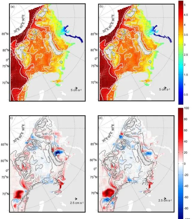
Fig. 9.Vertically integrated salt content (kg m−2, color contours on a logarithmic scale) and barotropic velocities (arrows) for(a)summer
and(b)winter from the fifth year of integration of the control model run (without tides). The velocity vectors are capped at 5 cm s−1. The
difference in vertically integrated salt content (kg m−2, color contours) and barotropic velocities (arrows) between the model run with tides
and the control run for(c)summer and(d)winter. The velocity vectors are capped at 2.5 cm s−1.
scale for both winter and summer. The distribution of this parameter is dominated by the water depth and there is there-fore very little difference between the winter and summer plots. The lower panels in Fig. 9 show the difference in mean salt content between the run with and without tides. Red colors indicate a greater salt content when tides are
in-cluded in the model. Large positive and negative salt anoma-lies at 70◦N in the Norwegian Sea dominate these plots.
following the path of the Norwegian Atlantic Current. The western sector of the Barents Sea, including the area around Svalbard, contains more salt after five years when tides are included. In contrast, the eastern Barents Sea has less salt when tides are included in the model. The persistent posi-tive salinity anomaly along the Russian coast seen in Fig. 8 is confirmed as a net increase in salt content (Fig. 9c and d). A complicated series of positive and negative salt anomalies are seen in the Kara Sea. However, tides do not cause signif-icant changes to any of the net salt fluxes into or out of the Kara Sea, so these salt anomalies indicate small shifts in the circulation patterns within the Kara Sea.
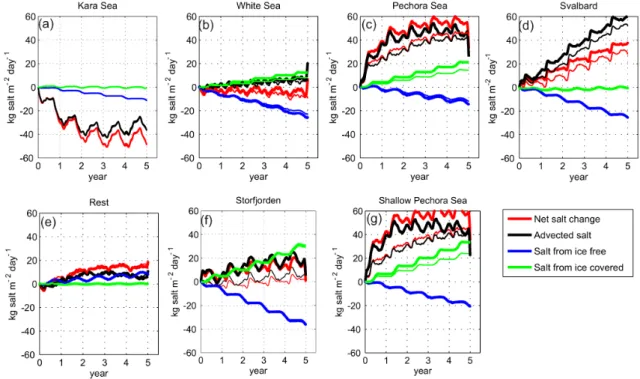
Clearly, the salt distribution of the model run with tidal forcing differs from the one without tides. The following analysis looks at how the vertically integrated salt content of the water column evolves throughout the duration of the model run. Comparing model output before it reaches steady state allows us to monitor how the two model runs diverge and diagnose the causes. Salt budgets for each region de-scribed in Sect. 3.2 along with two further subdomains (the shallow Pechora Sea – shallower than 50 m and Storfjorden – shallower than 100 m) are shown in Fig. 10a–g. Each subplot contains thin lines representing data from the control run and thick lines representing data from the model run including tides. In some cases the results for the two experiments are very similar so only the thick lines are visible. The day to day change in mean salt content of the regions has been at-tributed to three sources; lateral transport, surface salt fluxes from ice covered regions (brine rejection, sea ice/snow melt-ing and rain fallmelt-ing on ice) and surface salt fluxes from ice free regions (evaporation and precipitation over water). For clarity, we discuss each of these processes in turn.
4.1.1 Lateral advection of salt
Advection is the prime source or sink of salt in all shelf re-gions apart from the White Sea. Transport to the White Sea is restricted by a shallow channel which is only five grid cells wide, in contrast to the other subdomains which have long open boundaries across which salt can be advected. All sub-domains, apart from the Kara Sea, gain salt by lateral trans-port during the five years of the experiment. Salt transtrans-port between subdomains reaches steady state within 3 yr apart from in the Svalbard subdomain which is still gaining salt at the end of the five year run. Including tides in the model in-creases the mass of salt advected into the Pechora Sea and the Svalbard subdomains but the remaining regions show little change, reflecting the weakness of the tides there. Interest-ingly, in the Pechora Sea the mass of salt in the water column due to advection appears to be converging for the two model runs. Although the length of the model run does not allow us to confirm whether the salt transports from the two models do converge in this location, we suggest that including tides in the model decreases the time required to reach steady state for this parameter.
4.1.2 Surface salt fluxes from ice free areas
An imbalance between the amount of precipitation and evap-oration over ice free areas is also an important contributor to the evolution of the salt budget of the model. These param-eters are really freshwater fluxes but the POLCOMS model converts them to a salt flux and does not alter the water vol-ume. The blue line in Fig. 10 shows the change to the mass of salt associated with evaporation and precipitation over open water or leads within the ice cover. A seasonal cycle can be seen in all five shelf regions but the signal is dominated by ongoing trends. Four of the subdomains have a negative trend meaning that locally, the seasonal cycle of precipitation is outstripping that of evaporation causing the water column to freshen. Including tides in the model makes little differ-ence to the surface salt fluxes from ice free areas in any part of the model domain. As we saw in Sect. 3.2, including tides in the model leads to a decrease in ice concentration during the freeze up and melting season in the Pechora and White Seas. The associated increase in open water at these loca-tions allows increased ice production which is partially com-pensated by an increase in precipitation directly entering the ocean.
4.1.3 Surface salt fluxes from ice covered areas
Fig. 10.Time series of the change in vertically integrated salt content (kg salt m−2) relative to the initial salt content,S
0(red). Daily means
have been spatially averaged over the five subdomains shown in Fig. 2b and two additional subdomains; Storfjorden and the shallow Pechora Sea. The contribution to vertically integrated salt content from lateral advection (black), surface fluxes from ice free regions (blue) and surface fluxes from ice covered regions (green) are also shown. Thick lines show results from the model run including tides and thin lines are from the control run. A thirty day running mean has been applied to remove high frequency variation and highlight the trends. Initial values areS0=2714 kg m−2(Kara Sea), 1811 kg m−2(White Sea), 1379 kg m−2(Pechora Sea), 3883 kg m−2(Svalbard), 7862 kg m−2(Barents
Sea), 771 kg m−2(Storfjorden) and 708 kg m−2(shallow Pechora Sea).
the whole Svalbard subdomain. Indeed, the tidally induced change to salt content in this region is primarily due to an increase in the lateral advection of salt (Fig. 10d). However, when the domain is limited to the Storfjorden region, brine rejection clearly forms a major component of the salt budget (Fig. 10f). Brine rejection does not change significantly with the addition of tides in this location.
As mentioned above, the model predicts that the Pechora Sea is a net exporter of ice, which is transported into the Bar-ents Sea by the western Novaya Zemlya Current along the western coast of Novaya Zemlya (Panteleev et al., 2007) and the Kara Sea through the Kara Gate. This excess sea ice formation and export in the Pechora Sea provides a positive contribution to the annual salt budget of the region in both the tides and no-tides experiments but is stronger in the former run. Tides cause a residual current to flow from the entrance to the White Sea around the Kanin Peninsula (Fig. 8). This residual current could be due to tidal rectification or density driven by the increased salinity at the Kanin Peninsula. Dur-ing the summer this current extends all the way along the coast of the Pechora Sea to the entrance to the Kara Sea but is reduced in the winter. There is no change to the Novaya Zemlya Current with the inclusion of tides.
The part of the model where tides cause the most signifi-cant increase in salt due to excess brine rejection is the Pe-chora Sea. The details of the salt budget analysis presented here are sensitive to the location of the subdomain bound-aries. It was noted in Sect. 3.3 that the salinity increase in the Pechora Sea was most prominent shoreward of the 50 m bathymetric contour. The salt budget for this shallow sector of the Pechora Sea reveals that the large tidally induced in-crease in salinity here is driven primarily by inin-creased brine rejection (Fig. 10g). This region acts as a brine factory ex-porting ice and brine to the adjacent Pechora Sea and beyond.
5 Summary and conclusions
However, only the more tidally active sites, the Pechora Sea and the White Sea, saw a significant delay in freezing and a speed up of ice retreat during the melting season. Koentopp et al. (2005) also reached a similar conclusion in their model-ing study of tide/ice interaction in the Weddell Sea. Although including tides in the model leads to an increase in ice vol-ume around Svalbard for most of the year, this is not formed in situ but is advected in from outside. Hence there is no associated brine rejection signal associated with it.
Although we have not made any attempt to quantify whether including tides in the model better represents oceanographic observations, it is clear that omitting any rep-resentation of them from models will neglect many impor-tant physical processes. Parameterising tide-ice interactions such as in Holloway and Proshutinsky (2007) is a computa-tionally efficient way to proceed if fully resolving the tides is not possible. However, the parameterization described by Holloway and Proshutinsky (2007) does not capture the ef-fects of increased horizontal mixing or residual currents that we found to be significant in this study. Moreover, tides can create strong vertical current shear that increases vertical mixing, thus homogenizing the water column and bringing warm, saline Atlantic water towards the surface. This impor-tant process is represented in our model but is not discussed in the salt budget analysis as it has no net effect on the verti-cally integrated salt content.
In this study we have investigated whether the interaction between tides and sea ice has an impact on brine rejection. Two locations, the White and Pechora Seas, are key sites where brine rejection increases by 50% when tides are in-cluded in the model. Landfast ice is not represented in this study so it is likely that polynyas caused by offshore winds occur closer to the coast in these simulations than in ones which do include landfast ice. Locating the ice producing polynyas in more tidally active regions closer to the coast may mean the effect of tides on brine rejection is overesti-mated in this study. However, as the band of landfast ice is relatively narrow in the Pechora Sea it seems likely that the region would be a key site of enhanced brine rejection due to tide ice interaction irrespective of the presence of land fast ice. What distinguishes these two sites from other shal-low, tidally active locations is not clear. They do stand out as locations where adding tides to the model significantly re-duces the mixing parameterh/U3(wherehis the water depth andUis the depth mean current), indicating enhanced mix-ing (Simpson and Hunter, 1974). Hannah et al. (2009) used this parameter in the Canadian Arctic Archipelago to iden-tify recurrent sensible heat polynyas that are influenced by tidal currents. It is likely that there are other similar sites across the Arctic where increased brine rejection occurs due to tide/ice interaction.
Acknowledgements. This work was funded by the UK Natural Environment Research Council Strategic Research Programme Oceans 2025 and Thematic Programme RAPID, via Grant NER/T/S/2002/00979. We would like to thank Pam Posey and Lucy Smedstad from the Naval Research Laboratory for assistance in supplying NCOM and PIPS data for the boundary conditions for this study. ERA-40 data was kindly supplied by the European Centre for Medium-Range Weather Forecasts. We appreciate the comments of John Huthnance, Adrian Turner and an anonymous reviewer that greatly enhanced the paper.
Edited by: M. Hecht
References
Arbic, B. K., Wallcraft, A. J., and Metzger, E. J.: Concurrent sim-ulation of the eddying general circsim-ulation and tides in a global ocean model, Ocean Model., 32, 175–187, 2010.
Andreu-Burillo, I., Holt, J., Proctor, R., Annan, J. D., James, I. D., and Prandle, D.: Assimilation of sea surface temperature in the POL Coastal Ocean Modelling System, J. Marine Syst., 65, 27– 40, 2007.
Barron, C. N., Kara, A. B., Martin, P. J., Rhodes, R. C., and Smed-stad, L. F.: Formulation, implementation and examination of ver-tical coordinate choices in the Global Navy Coastal Ocean Model (NCOM), Ocean Model., 11, 347–375, 2006.
Barron, C. N., Kara, A. B., Rhodes, R. C., Rowley, C., and Smed-stad, L. F.: Validation Test Report for the 1/8 Global Navy Coastal Ocean Model Nowcast/Forecast System, NRL Report NRL/MR/7320–07-9019, Stennis Space Center, MS, 2007. Cavalieri, D., Parkinson, C., Gloersen, P., and Zwally, H. J.: Sea ice
concentrations from Nimbus-7 SMMR and DMSP SSM/I pas-sive microwave data, (September 2000, March 2001) Boulder, Colorado USA: National Snow and Ice Data Center, Digital me-dia, 1996, updated 2008.
Egbert, G. D. and Erofeeva, S. Y.: Efficient inverse modeling of barotropic ocean tides, J. Atmos. Ocean. Tech., 19, 183–204, 2002.
Egbert, G. D. and Ray, R. D.: Significant dissipation of tidal energy in the deep ocean inferred from satellite altimeter data, Nature, 405, 775–778, 2000.
Eisen, O. and Kottmeier, C.: On the importance of leads in sea ice to the energy balance and ice formation in the Weddell Sea, J. Geophys. Res.-Oceans, 105, 14045–14060, 2000.
Gjevik, B. and Straume, T.: Model simulations of the M2 and the K1 tide in the Nordic Seas and the Arctic Ocean, Tellus, 41A, 73–96, 1989.
GRDC: River discharge data 1954–1999, Global Runoff Data Cen-tre, Koblenz, 56068 Germany, 2003.
Hannah, C. G., Dupont, F., and Dunphy, M.: Polynyas and Tidal Currents in the Canadian Arctic Archipelago, Arctic, 62, 83–95, 2009.
Holloway, G. and Proshutinsky, A.: The role of tides in Arctic ocean/ice climate, J. Geophys. Res., 112, C04S06, doi:10.1029/2006JC003643, 2007.
Prog. Oceanogr., 60, 47–98, 2004.
Kern, S., Kaleschke, L., and Spreen, G.: Climatology of the Nordic (Irminger, Greenland, Barents, Kara and White/Pechora) Seas ice cover based on 85 GHz satellite microwave radiometry: 1992–2008, Tellus A, 62A, 411–434, 2010.
Koentopp, M., Eisen, O., Kottmeier, C., Padman, L., and Lemke, P.: Influence of tides on sea ice in the Weddell Sea: Investigations with a high-resolution dynamic-thermodynamic sea ice model, J. Geophys. Res., 110, C02014, doi:10.1029/2004JC002405, 2005. Kowalik, Z. and Proshutinsky, A. Y.: The Arctic Ocean tides, in: The polar oceans and their role in shaping the global environ-ment: the Nansen centennial volume, edited by: Johannessen, O. M., Muench, R. D., and Overland, J. E., 525 pp., 1994.
Kowalik, Z. and Proshutinsky, A. Y.: Topographic enhancement of tidal motion in the western Barents Sea, J. Geophys. Res., 100, 2613–2637, 1995.
Lenn, Y.-D., Rippeth, T. P., Old, C. P., Bacon, S., Polyakov, I., Ivanov, V., and H¨olemann, J.: Intermittent intense turbulent mixing under ice in the Laptev Sea Continental Shelf, J. Phys. Oceanogr., doi:10.1175/2010JPO4425.1, in press, 2010. Martin, S., Polyakov, I., Markus, T., and Drucker, R.: Okhotsk Sea
Kashevarov Bank polynya: Its dependence on diurnal and fort-nightly tides and its initial formation, J. Geophys. Res.-Oceans, 109, C09S04, doi:10.1029/2003JC002215, 2004.
Maykut, G. A.: Large-Scale Heat-Exchange and Ice Production in the Central Arctic, J. Geophys. Res.-Oc. Atm., 87, 7971–7984, 1982.
Maykut, G. A. and Perovich, D. K.: The Role of Shortwave Ra-diation in the Summer Decay of a Sea Ice Cover, J. Geophys. Res.-Oceans, 92, 7032–7044, 1987.
Mellor, G. L. and Yamada, T.: Hierarchy of Turbulence Clo-sure Models for Planetary Boundary-Layers, J. Atmos. Sci., 31, 1791–1806, 1974.
Midttun, L.: Formation of dense bottom water in the Barents Sea, Deep-Sea Res., 32, 1233–1241, 1985.
Morales-Maqueda, M. A., Willmott, A. J., and Biggs, N. R. T.: Polynya Dynamics: A review of observations and modeling, Rev. Geophys., 42, RG1004, doi:10.1029/2002RG000116, 2004. Muller, M., Haak, H., Jungclaus, J. H., S¨undermann, J., and
Thomas, M.: The effect of ocean tides on a climate model simu-lation, Ocean Model., 35, 304–313, 2010.
Munk, W. and Wunsch, C.: Abyssal Recipes II: energetics of tidal and wind mixing, Deep-Sea Res. Pt. I, 45, 1977–2010, 1998. Padman, L. and Erofeeva, S.: A barotropic inverse tidal model
for the Arctic Ocean, Geophys. Res. Lett., 31, L02303,
Sumi, A., and Taylor, K. E.: Climate Models and their Evalu-ation, in: Climate Change 2007 – The Physical Science Basis. Contribution of Working Group I to the fourth Assessment Re-port of the Intergovernmental Panel on Climate Change, edited by: Solomon, S., Qin, D., Manning, M., Chen, Z., Marquis, M., Averyt, K. B., Tignor, M., and Miller, H. L., Cambridge Uni-versity Press, Cambridge, United Kingdom and New York, NY, USA, 2007.
Rippeth, T.: Mixing in seasonally stratified shelf seas: a shifting paradigm, Philos. T. R. Soc. A, 363, 2837–2854, 2005.
Rudels, B., Jones, E. P., Anderson, L. G., and Kattner, G.: On the Intermediate Depth Waters of the Arctic Ocean, in: The Polar Oceans and Their Role in Shaping the Global Environment, Geo-physical Monograph 85, edited by: Johannessen, O. M., Muench, R. D., and Overland, J. E., AGU, Washington, 33–46, 1994. Schauer, U., Loeng, H., Rudels, B., Ozhigin, V. K., and Dieck, W.:
Atlantic Water flow through the Barents and Kara Seas, Deep-Sea Res. Pt. I, 49, 2281–2298, 2002.
Serreze, M. C. and Hurst, C. M.: Representation of mean Arctic pre-cipitation from NCEP-NCAR and ERA reanalyses, J. Climate, 13, 182–201, 2000.
Serreze, M. C., Barrett, A. P., Slater, A. G., Steele, M., Zhang, J., and Trenberth, K. E.: The large-scale energy budget of the Arc-tic, J. Geophys. Res., 112, D11122, doi:10.1029/2006JD008230, 2007.
Sharples, J., Moore, C. M., and Abraham, E. R.: Internal tide dis-sipation, mixing, and vertical nitrate flux at the shelf edge of NE New Zealand, J. Geophys. Res., 106, 14069–14081, 2001. Siddorn, J. R., Allen, J. I., Blackford, J. C., Gilbert, F. J., Holt, J.
T., Holt, M. W., Osborne, J. P., Proctor, R., and Mills, D. K.: Modelling the hydrodynamics and ecosystem of the North-West European continental shelf for operational oceanography, J. Ma-rine Syst., 65, 417–429, 2007.
Simpson, J. H. and Hunter, J. R.: Fronts in the Irish Sea, Nature, 250, 404–406, 1974.
Song, Y. H. and Haidvogel, D.: A Semi-implicit Ocean Circulation Model Using a Generalized Topography-Following Coordinate System, J. Comput. Phys., 115, 228–244, 1994.
Thomas, M. and S¨undermann, J.: Consideration of ocean tides in an OGCM and impacts on subseasonal to decadal polar motion excitation, Geophys. Res. Lett., 28, 2457–2460, 2001.
Beljaars, A. C. M., van de Berg, L., Bidlot, J., Bormann, N., Caires, S., Chevallier, F., Dethof, A., Dragosavac, M., Fisher, M., Fuentes, M., Hagemann, S., H´olm, E., Hoskins, B. J., Isak-sen, L., JansIsak-sen, P. A. E. M., Jenne, R., McNally, A. P., Mahfouf, J.-F., Morcrette, J.-J., Rayner, N. A., Saunders, R. W., Simon, P., Sterl, A., Trenberth, K. E., Untch, A., Vasiljevic, D., Viterbo, P., and Woollen, J.: The ERA-40 re-analysis, Q. J. Roy. Meteor. Soc., 131, 2961–3012, 2005.
Willmott, A. J., Holland, D. M., and Morales Maqueda, M. A.: Polynya modeling, in: Polynyas: Windows to the World, edited by: Smith Jr., W. O. and Barber, D. G., Elsevier, Oxford, (Else-vier Oceanography Series, 74) 87–125, 2007.