www.hydrol-earth-syst-sci.net/18/305/2014/ doi:10.5194/hess-18-305-2014
© Author(s) 2014. CC Attribution 3.0 License.
Hydrology and
Earth System
Sciences
Addressing drought conditions under current and future climates in
the Jordan River region
T. Törnros and L. Menzel
Institute of Geography, Heidelberg University, Heidelberg, Germany
Correspondence to:T. Törnros ([email protected])
Received: 2 April 2013 – Published in Hydrol. Earth Syst. Sci. Discuss.: 7 May 2013 Revised: 3 December 2013 – Accepted: 5 December 2013 – Published: 23 January 2014
Abstract. The Standardized Precipitation–Evaporation In-dex (SPEI) was applied in order to address the drought con-ditions under current and future climates in the Jordan River region located in the southeastern Mediterranean area. In the first step, the SPEI was derived from spatially interpo-lated monthly precipitation and temperature data at multi-ple timescales: accumulated precipitation and monthly mean temperature were considered over a number of timescales – for example 1, 3, and 6 months. To investigate the perfor-mance of the drought index, correlation analyses were con-ducted with simulated soil moisture and the Normalized Dif-ference Vegetation Index (NDVI) obtained from remote sens-ing. A comparison with the Standardized Precipitation Index (SPI), i.e., a drought index that does not incorporate tem-perature, was also conducted. The results show that the 6-month SPEI has the highest correlation with simulated soil moisture and best explains the interannual variation of the monthly NDVI. Hence, a timescale of 6 months is the most appropriate when addressing vegetation growth in the semi-arid region. In the second step, the 6-month SPEI was de-rived from three climate projections based on the Intergov-ernmental Panel on Climate Change emission scenario A1B. When comparing the period 2031–2060 with 1961–1990, it is shown that the percentage of time with moderate, se-vere and extreme drought conditions is projected to increase strongly. To address the impact of drought on the agricultural sector, the irrigation water demand during certain drought years was thereafter simulated with a hydrological model on a spatial resolution of 1 km. A large increase in the demand for irrigation water was simulated, showing that the agricul-tural sector is expected to become even more vulnerable to drought in the future.
1 Introduction
Drought is an extended period with water deficits. Different kinds of drought include meteorological, hydrological and agricultural drought (Wilhite and Glantz, 1985). A meteo-rological drought is related to abnormally low precipitation, typically over an extended period of time. Although factors like temperature, wind speed and soil conditions also are of importance, a meteorological drought can trigger both hy-drological droughts (abnormally low lake levels or river dis-charge) and agricultural droughts (abnormally low soil mois-ture). In many parts of the world, drought is a recurrent nat-ural hazard that has environmental, social and economic im-pacts (Wilhite, 2005). This wide range of imim-pacts can be sim-plified and quantified with a drought index. Through such an index, current and past drought events can be compared and essential communication between scientist, decision makers and the public facilitated (Wilhite et al., 2000).
Crop Moisture Index (CMI; Palmer, 1968). The CMI is in general applied in order to address short-term droughts on a week-to-week basis. An advantage of the PDSI and CMI is that they can address the soil moisture status of a region. However, this also implies high data requirements and a high number of defined terms (Alley, 1984; Paulo and Pereira, 2006). Hence, there is also a need for simpler drought in-dices, relying on fewer data and fewer calculations (Hayes et al., 1999; Smith et al., 1993). The Australian Bureau of Meteorology favors the drought index deciles where precip-itation is ranked from lowest to highest and split into 10 groups (Gibbs and Maher, 1967). The index is easy to cal-culate and provides an estimation of how rare certain precip-itation amounts are in comparison to the mean. Nonetheless, a long data record is required (Quiring, 2009). Another well-known drought index is the Standardized Precipitation Index (SPI), developed by McKee et al. (1993) and applied world-wide. The index uses long data records of precipitation as the only input, and in contrast to other drought indices, the SPI can be applied on different timescales (e.g., 1, 3, or 6 months) in order to address the accumulation periods between pre-cipitation and the water supplies in soil moisture, ground-water, snowpack, streamflow and reservoir storage (McKee et al., 1993). The SPI has been recommended by the World Meteorological Organization (WMO, 2011) for characteriz-ing meteorological droughts. An advantage of the SPI is the low amount of required input parameters (only precipitation). Some critics are concerned that the index does not perform well at precipitation near zero (Wu et al., 2007) and that the effect of evapotranspiration is not considered (Vicente-Serrano et al., 2010). To address the latter, there is also a further development of SPI, the Standardized Precipitation– Evaporation Index (SPEI), which incorporates temperature for the calculation of potential evapotranspiration (Vicente-Serrano et al., 2010). In a global assessment of different drought indices, Vicente-Serrano et al. (2012) conclude that the SPI and SPEI are superior to the PDSI in capturing the drought impacts on hydrological, agricultural and ecological variables.
Although the link between precipitation, soil moisture and vegetation growth is widely recognized (Farrar et al., 1994; Gu et al., 2008; Wang et al., 2007), the soil moisture data are often limited to point measurements. Higher data avail-ability is one of the reasons why other studies have focused on the indirect relationship between precipitation and motely sensed data on vegetation in arid and semi-arid re-gions (Anyamba and Tucker, 2005; Fabricante et al., 2009; Nicholson and Farrar, 1994; Nezlin et al., 2005; Schmidt and Karnieli, 2000). Such an analysis offers the opportunity to address the performance of a drought index; a positive cor-relation between a drought index and a vegetation index in-forms about the drought index’s capability of addressing the agricultural response to drought (Ji and Peters, 2003; Quiring and Ganesh, 2010; Vicente-Serrano et al., 2012). One of the most used vegetation indices is the Normalized Difference
Vegetation Index (NDVI) derived from spectral reflectance in the near-infrared (NIR) and visible red regions according to
NDVI=(ρNIR−ρRed)/(ρNIR+ρRed), (1) whereρNIRandρRedare the reflectance at the NIR and vis-ible red bands. The NDVI can be obtained from the Ad-vanced Very High Resolution Radiometer (AVHRR) and Moderate Resolution Imaging Spectroradiometer (MODIS) sensors, among others (Tucker et al., 2005), and be used as an estimate of biomass and net primary production (Leprieur et al., 2000).
Many studies have addressed future drought conditions and water stress (Burke and Brown, 2010; Dai, 2011; Milano et al., 2012; Li et al., 2008). By applying a well-performing drought index, not only the characteristics of current and past drought events can be determined, but in combination with climate projections, future conditions can also be ad-dressed. Several authors have made projections of future changes in the eastern Mediterranean climate by applying global climate models (GCMs) and regional climate models (RCMs). Krichak et al. (2011) applied an ECHAM5/MPI-OM RegCM3 model and noticed a significant trend of de-creasing winter precipitation in near-coastal areas and an in-creasing trend in air temperature for all seasons. Samuels et al. (2011) applied the ECHAM5 and HadCM3 GCMs in combination with the RegCM3 and MM5 RCMs. Their re-sults showed that the maximum daily temperature is expected to increase by 2.5–3◦
C and that the lengths of warm and dry spells are expected to be prolonged by 2021–2050 compared with the control period of 1961–1990. Smiatek et al. (2011) applied the ECHAM-MM5 and HADCM3-MM5 projections and identified a 2.1◦
C mean increase of the annual mean temperature by 2031–2060 compared with 1961–1990. They also identified a drop in the annual mean precipitation by 11.5 %. Together, the application of regional climate mod-els has shown that the eastern Mediterranean climate is pro-jected to become warmer and drier. In order to develop sound water management strategies and preparedness for drought, it is meaningful to address the drought characteristics un-der a changing climate. Further applications of a hydrolog-ical model can thereafter be used to simulate the impact of drought on the agricultural sector in a more detailed manner. Considering that this sector accounts for 58 % of the regional water use (FAO, 2009), the results would especially be use-ful for stakeholders and decision makers when developing a long-term regional drought preparedness plan.
as well as the precipitation-based SPI. Also drought char-acteristics are addressed; the drought indices are applied both on climate model control data as well as on climate data received from future projections. Comparisons are also made with observed reference data. Thereafter, a hydrolog-ical model is used to simulate the irrigation water demand (IWD) during extreme droughts. In that way, the simulated IWD can be used to address the impact of climate change on the agricultural sector. More in detail, the focus is on the following: (1) the correlation between multiple timescales of SPEI and SPI, simulated soil moisture and monthly NDVI in order to identify the SPEI and SPI timescale that best ex-plains the vegetation dynamics in the wider Jordan River re-gion; (2) deriving the percentage of time with moderate, se-vere and extreme drought conditions under current and future climates; and (3) simulating the IWD during a current and fu-ture drought year in order to address the agricultural impacts of a changing climate.
2 Materials and methods
2.1 Study region
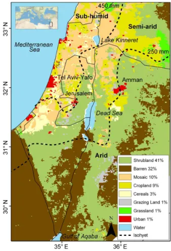
The present study region covers the Jordan River basin and its surroundings (Fig. 1). The area extends from north of Lake Kinneret to the Gulf of Aqaba in the south, and from the Mediterranean coast to the Jordanian Highlands in the east. Altogether, the study area covers around 96 000 km2 and includes Israel, the State of Palestine, and a major part of Jordan, as well as parts of Lebanon, Syria, and Egypt. The region is characterized by a wet season between October and April, whereas the rest of the year receives no precipi-tation. On an annual basis, the potential evaporation greatly exceeds precipitation. The interannual variability of winter precipitation is strong, and abnormally low rainfall recur-rently triggers drought events resulting in economic losses, lowered agriculture productivity, reduced stream flow, and falling lake levels (Inbar and Bruins, 2004). In addition, the spatial variability of precipitation is high; convective storms are common, and two significant precipitation gradients ex-ist (Ben-Gai et al., 1998). The first gradient is in the west– east direction with higher precipitation in proximity to the Mediterranean Sea (Fig. 1). The hilly regions, stretching from Lebanon in the north to the Gulf of Aqaba in the south, give rise to an orographic lift of moist westerly winds, which results in a dry eastern lee side (Dahamsheh and Aksoy, 2007). The second gradient is in the north–south direction. The Golan Heights, stretching northwards from the eastern side of Lake Kinneret, have humid conditions with an annual precipitation of up to 900 mm. Around the Gulf of Aqaba, the conditions are hyper-arid. The area receives dry winds from the Sinai desert, and the annual precipitation is less than 50 mm (Dahamsheh and Aksoy, 2007).
Fig. 1.Location of the study region (based on the ESRI World Phys-ical Map) and land uses with spatial coverage in percentages. Also shown are the 250 and 450 mm isohyets derived from spatially in-terpolated precipitation data. These smoothed lines define a sub-humid, semi-arid and arid sub-region.
2.2 SPEI and SPI
The drought index SPEI (Vicente-Serrano et al., 2010) is a further development of the SPI described in detail by McKee et al. (1993), Guttman (1999) and Bordi et al. (2001). The focus of this paper is on the SPEI; nonetheless, comparisons are conducted with the SPI. The original SPI uses long-term precipitation series, preferably not shorter than 30 yr, as only input (McKee et al., 1993). The SPEI instead requires a series of the climate water balance (precipitation – potential evapo-ration) as input (Beguería and Vicente-Serrano, 2013). Here we applied the Thornthwaite equation (Thornthwaite, 1948), which employs the latitude and the monthly average temper-ature in order to estimate the potential evaporation. To begin the calculations of the SPEI and SPI, a probability density function is fitted to the long-term input series for a certain timescale of interest. The fit is conducted separately for each month of the year, and the series is a running time series of for example a 1-, 3- or 6-month cumulative climate water bal-ance for the SPEI and cumulative series of precipitation for the SPI. The probability density function is thereafter trans-formed to a standard normal distribution with the mean value of 0 and standard deviation of 1. According to the original definition by McKee et al. (1993), drought conditions occur when the SPI is continuously negative and falls below a cer-tain threshold value. The authors suggested a threshold value of −1 for moderate drought; the SPEI and SPI values are expected to be below this threshold 15.9 % (1 standard devi-ation) of the time.
For the purpose of this study, the SPEI and SPI were cal-culated with the SPEI R package (Beguería and Vicente-Serrano, 2013). When calculating the SPEI, the log-logistic probability density function was used. When deriving the SPI, the gamma probability density function was instead em-ployed. Both the SPEI and SPI were applied on gridded data where each 1 km×1 km pixel acted as a single measurement point.
2.3 Time series of SPEI, SPI and NDVI
Precipitation and temperature were interpolated to a spa-tial resolution of 1 km by using data obtained for the pe-riod 1961–2001 from more than 130 precipitation gauges and around 50 temperature sensors. The spatial resolution was chosen to coincide with the land use map. To account for the strong climatic gradients and an irregular spatial distribu-tion of the stadistribu-tions, a multiple regression analysis, described in detail in Menzel et al. (2009) and Wimmer et al. (2009), was applied. Based on the daily data availability, data char-acteristics and possible spatial trends, the method automat-ically identifies a suitable interpolation method (universal kriging, ordinary kriging, ordinary least squares interpolation or inverse distance weighting) for each day and parameter. Thereafter, the interpolated daily precipitation and tempera-ture grids were aggregated into monthly totals and monthly
mean values, respectively. These grids served as input to the SPEI and SPI.
In order to identify the most appropriate SPEI and SPI timescale, the drought indices were applied on short timescales (1, 2, and 3 months), moderate timescales (6, 9, and 12 months), as well as long timescales (18 and 24 months) for each pixel separately. During the SPEI and SPI calculations, the input series were then accumulated to this timescale and compared with the corresponding period in the long-term climatic series. As an example, to derive the 3-month SPEI value of March 2000 for a pixel, the total cli-mate water balance of January, February and March 2000 was compared (standardized) with long-term time series of January–March climate water balance for the same pixel. Throughout the whole study, the gridded observed data for 1961–1990 were used as reference data. Hence, the observed data were used for standardization. The final monthly SPEI and SPI data sets had a spatial resolution of 1 km.
2.4 Climate projections
Once the SPEI and SPI had been compared and the most suitable timescale had been identified based on regression analysis between the drought indices, simulated soil mois-ture and NDVI, data from three climate projections were applied in order to address future droughts. The Intergov-ernmental Panel on Climate Change (IPCC) has prepared several emission scenarios in order to address uncertain-ties in global development. In the present study, we apply the emission scenario A1B, which describes a world with a very rapid economic growth and where energy is generated both from fossil fuels and from alternative energy sources (IPCC, 2007). Three combinations of a GCM and RCM, prepared within the GLOWA Jordan River Project (http: //www.glowa-jordan-river.de/), were considered: ECHAM5-MM5 and HadCM3-ECHAM5-MM5 (Samuels et al., 2011; Smiatek et al., 2011) delivered from the Institute for Meteorology and Climate Research – Atmospheric Environmental Research (IMK-IFU) in Karlsruhe, Germany, and ECHAM5-RegCM3 (Krichak et al., 2010, 2011) delivered from the Tel Aviv Uni-versity (TAU), Israel. Not all RCMs are appropriate for each region (Krichak et al., 2010). The applied RCMs, however, have been adapted and optimized for the eastern Mediter-ranean region (Krichak et al., 2005, 2007).
The climate projections have spatial resolutions of 18– 25 km. From the projections, daily precipitation and tem-perature data were disaggregated to a spatial resolution of 1 km by applying a linear interpolation between the center points of each grid cell. Following this, monthly values were retrieved, and the best performing drought index was ap-plied to the climate model control run (1961–1990) and fu-ture projections (2031–2060) by using the gridded observed data 1961–1990 as a reference. In order to compare the dif-ferent time periods with regards to drought, the SPEI and SPI probability density functions were derived by using all pixels for all months (altogether 96 318 pixels×360 months for each time period). By applying this method, it was pos-sible to derive the percentage of time of moderate drought (SPEI/SPI <−1.0), severe drought (SPEI/SPI <−1.5) and extreme drought (SPEI/SPI <−2.0) conditions.
2.5 Hydrological model
TRAIN is a physically based hydrological model that has fo-cus on the soil–vegetation–atmosphere interface. It is based on comprehensive field studies regarding the water and en-ergy balance of different surface types, including natural veg-etation and agricultural land (Menzel, 1997a, b). Recently, the model has been calibrated with evapotranspiration mea-sured in the semi-arid Yatir Forest, Israel (Hausinger, 2009), a research site operated by the Weizmann Institute of Sci-ence. Furthermore, the model has been applied in several studies focusing on the water balance in the wider Jordan River region (Menzel et al., 2009; Menzel and Törnros, 2012;
Törnros and Menzel, 2014). The model requires input data on precipitation, temperature, wind speed, radiation, and air humidity. These data were available both from meteorologi-cal stations and from climate projections, and were prepared just as the precipitation and temperature grids. TRAIN also requires information regarding land use and the water hold-ing capacities of the soils. These data were available from the International Geosphere-Biosphere Programme GLCC (Loveland et al., 2000; Menzel et al., 2009) and Schacht et al. (2011), respectively.
Based on the necessary input data, TRAIN simulates soil moisture, evapotranspiration, snow accumulation/melt, runoff and percolation. For agricultural areas, TRAIN can also deliver information regarding the irrigation water de-mand (IWD). The model presumes that optimal crop growth takes place when the soil is saturated to field capacity. When the simulated soil moisture drops below a certain threshold level, the model simulates irrigation until optimal plant con-ditions (field capacity) are reached. The derived IWD is of potential value. In reality, and especially during droughts and water shortages, a sufficient amount of water might not be allocated to agriculture. In the present study, TRAIN was applied to simulate soil moisture for the sake of addressing the SPEI/SPI–soil moisture–NDVI relation. In addition, the model was also applied in order to simulate the IWD during average reference conditions and drought years. The latter was defined as the year having the highest drought magni-tude (monthly accumulated negative SPEI/SPI over the year) according to McKee et al. (1993). The result can be used as an indicator of the drought vulnerability of the region. The higher the IWD, the more threatened the agricultural sector becomes because more water is required to sustain (optimal) vegetation growth.
3 Results
3.1 Spatiotemporal variability of NDVI
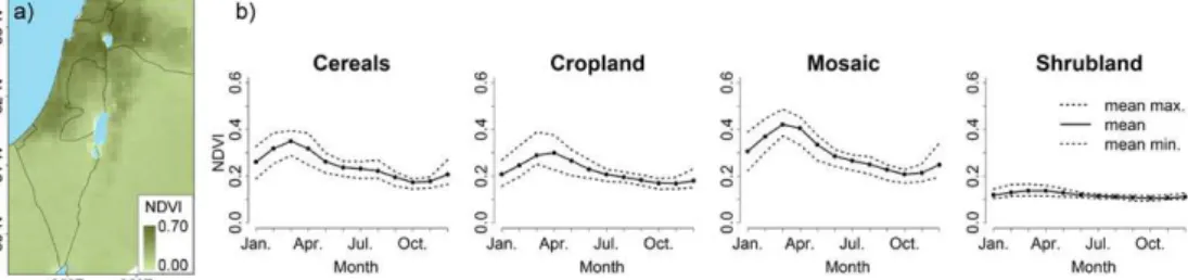
Fig. 2. (a)Spatial distribution of NDVI in April 2000, and(b)the NDVI phenology throughout the year for chosen land uses. Shown are the maximum mean NDVI, the mean NDVI, and the minimum mean NDVI based on monthly values for the years 1982–2001.
also highlights a clear vegetation peak in March/April. By conducting regression analyses between NDVI and multiple timescales of the SPEI and SPI, it was tested whether the drought indices could explain these interannual variations in vegetation.
3.2 Correlation of SPEI, SPI and NDVI
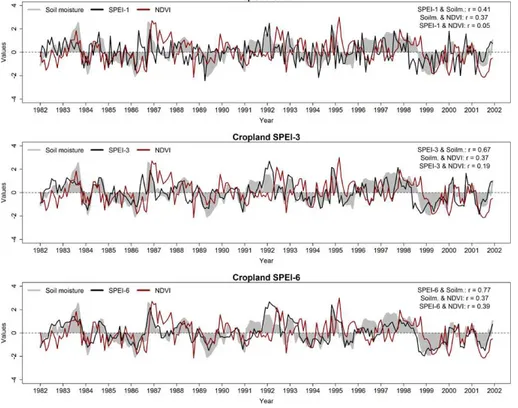
For each considered land use (cereals, cropland, mosaic and shrubland), correlation analyses were conducted be-tween multiple timescales of the SPEI/SPI, soil moisture and NDVI. Figure 3 shows some of the derived time series for cropland. By examining the 1-month SPEI, it becomes clear that the drought conditions quickly change between months and that the response in soil moisture is slower. This result in a moderate correlation between the parameters (r=0.41). Between the 3-month SPEI and soil moisture, the correla-tion is increased (r=0.67). Nonetheless, the highest correla-tion is obtained between the 6-month SPEI and soil moisture (r=0.77). By examining these time series, it can be seen that the response times to an event tend to be comparable for the 6-month SPEI and soil moisture. It can also be seen that the 6-month SPEI and NDVI have a correlation coefficient of 0.39. This relation was addressed more in detail by inves-tigating the variations throughout the main growing season (January to May).
Figure 4 shows scatterplots of the NDVI and the 1-, 3- and 6-month SPEI (the other considered SPEI timescales are not plotted). The results demonstrate that little (significant) cor-relation is detected between NDVI and the 1-month SPEI. The relationship is furthermore only positive in March and April; during this month thepvalue (for the positive rela-tions) is between 0.38 and 0.95. It is clear that the 3-month SPEI shows a higher correlation with NDVI. The correla-tion is strongest, and at times significant (p< 0.05), in Jan-uary and during the vegetation peak in April/May. It can also be seen that a negative relation is obtained in Febru-ary and March. Furthermore, the results demonstrate that the 6-month SPEI performs better in comparison to the shorter timescales. Every month induces a positive correlation be-tween the 6-month SPEI and NDVI, and at the most, a corre-lation coefficient of 0.75 is obtained. In January the correla-tion is significant for cereals, and in February it is significant
for shrubland. In March it is significant both for cereals and shrubland, and in April and May it tends to be significant for all land uses. From all the scatterplots, it can be seen that the relationship between the NDVI and SPEI changes with the different states of vegetation growth. In general, it can also be seen that the correlation between the two parameters is strongest around the vegetation peak.
To facilitate the evaluation of all considered SPEI timescales and allow a comparison with SPI, the 20 regres-sion analyses (which were visualized with scatterplots) con-ducted for each timescale were evaluated with a box plot (Fig. 5). As the 1-month SPEI induces a negative correla-tion (r= −0.09) on average, the result once again indicates that the shortest timescale is not capable of monitoring veg-etation growth. The 2-month SPEI and 3-month SPEI have a higher average correlation (r=0.06 andr=0.26, respec-tively), probably because there is a time lag between precipi-tation and vegeprecipi-tation growth, and the impact of water deficits on vegetation is cumulative (Ji and Peters, 2003). The same figure shows that all moderate timescales perform almost equally well; the 6-, 9-, and 12-month SPEIs have an aver-age correlation coefficient of 0.49, 0.46, and 0.41, respec-tively. The box plot also reveals that the longer timescales tend to result in a lower correlation coefficient than the mod-erate timescales; the 18-month SPEI has an average corre-lation coefficient of 0.28, and the 24-month SPEI has a cor-responding value of 0.22. In the figure, it can also be seen that the SPEI tends to perform slightly better than the SPI, which only uses precipitation as input. For the SPI, the mod-erately long timescales perform almost equally well, having an average correlation coefficient between 0.44 and 0.47.
Altogether, the 6-month SPEI best explains the interannual variability of the monthly NDVI. Therefore, this timescale was chosen as the most appropriate for assessing agricultural drought in the Jordan River region.
3.3 Droughts under current and future climate conditions
Fig. 3.Time series of simulated soil moisture, NDVI and multiple timescales of the SPEI;rrefers to the correlation coefficient.
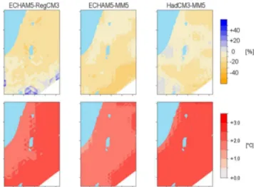
combinations all simulate a decrease of annual precipitation. For large areas, a decrease of between 10 to 20 % is pro-jected. The ECHAM5-RegCM3 simulates mainly a decrease in the semi-arid and sub-humid regions. There are also some local areas where increased precipitation is simulated, possi-ble owing to convective rainfall events (Samuels et al., 2011). Both the ECHAM5-MM5 and the HadCM3-MM5 simulate mainly a decrease in the southern arid parts. Although the spatial distributions of changes in annual precipitation differ slightly between the models, the results can give a sense of the range of the changes expected (Samuels et al., 2011). Fur-thermore, the projections give indications of a seasonal shift (not shown). Precipitation is projected to increase slightly during October to November, in the beginning of the wet sea-son. During the mid-winter months of December to February, a clear reduction in total precipitation is simulated. For the ECHAM5-RegCM3, the reduction is large for all the mid-winter months, whereas the ECHAM5-MM5 model simu-lates the strongest reduction in February and none in Jan-uary. In contrast, the HadCM3-MM5 simulates a reduction in January’s precipitation and only minor changes in Febru-ary. Furthermore, all climate projections predict a decrease in precipitation for March through May.
By 2031–2060, an increase of temperature by 1.5–2.0◦C is simulated; the highest increase is simulated by HadCM3-MM5 followed by RegCM3 and ECHAM5-MM5, respectively. As also noticed by Samuels et al. (2011), all models show a higher temperature increase inland than at
the coast. The authors suggest that it could be related to cool-ing effects of sea breezes. When examincool-ing the simulated change of monthly mean temperature throughout the wet sea-son, the results give an increase by 1.5–3◦
C (not shown). The increase tends to be highest in the beginning of the wet season. Increased temperature means a higher atmospheric evaporation demand and may have negative consequences for the agricultural sector.
Fig. 4.Scatterplots between NDVI and multiple timescales of SPEI for chosen land uses. Each dot represents one year between 1982 and 2001. Also shown are the correlation coefficientrand thepvalue.
Fig. 5.Box plot for the correlation of NDVI and multiple timescales of SPEI and SPI;ris the correlation coefficient. The figure is based on the months January to May, and the land uses cereals, cropland, mosaic and shrubland. Hence, altogether there are 20 values for each timescale.
the drought conditions in comparison to the reference data. Although the climate model control runs show biases when compared to the reference data, a comparison between the fu-ture projections and the control run can nonetheless reveal an indication of the expected changes with regards to drought. A first glance shows that the future projections have shifted towards more negative values in comparison to the control data. This means that SPEI and SPI are expected to be below
−1 more frequently.
Tables 1–2 show the percentage of time (equal to the percentage of months) with moderate, severe and extreme drought conditions. When evaluating the 6-month SPEI and the 6-month SPI (once again given in brackets), the results show that moderate drought occurs 9.0 % (8.7 %) of the time for the reference data. Severe and extreme droughts occur 4.2 % (3.8 %) and 2.0 % (1.7 %) of the time, respectively. Al-together this sums to 15.2 % (14.2 %), which is slightly lower than the 15.9% that is expected for a normal distribution with
Fig. 6.Projected relative changes in annual precipitation (upper row) and annual mean temperature (lower row) simulated by three climate models. The figure shows projected data for 2031–2060 in comparison with the climate model control run 1961–1990.
Table 1.The percentage of time with moderate, severe and extreme drought conditions as derived with the 6-month SPEI. The values are standardized according to the reference period 1961–1990 (observed data). “Ctrl.” refers to the climate model control run (1961–1990) and “Proj.” to the future projection (2031–2060).
Drought Reference ECHAM5-RegCM3 ECHAM5-MM5 HadCM3-MM5 SPEI Values condition 1961–1990 Ctrl. Proj. Ctrl. Proj. Ctrl. Proj.
−1.00 to−1.49 Moderate 9.0 % 9.1 % 13.0 % 10.2 % 13.2 % 5.2 % 12.9 %
−1.50 to 1.99 Severe 4.2 % 6.3 % 12.7 % 7.0 % 12.8 % 3.0 % 11.0 % ≤ −2.0 Extreme 2.0 % 7.7 % 33.9 % 8.1 % 33.7 % 2.5 % 21.3 %
Total: 15.2 % 23.1 % 59.6 % 25.3 % 59.7 % 10.7 % 45.2 %
Table 2.The percentage of time with moderate, severe and extreme drought conditions as derived with the 6-month SPI. The values are standardized according to the reference period 1961–1990 (observed data).
Drought Reference ECHAM5-RegCM3 ECHAM5-MM5 HadCM3-MM5 SPI Values condition 1961–1990 Ctrl. Proj. Ctrl. Proj. Ctrl. Proj.
−1.00 to−1.49 Moderate 8.7 % 9.4 % 10.2 % 11.6 % 12.0 % 11.5 % 11.7 % −1.50 to 1.99 Severe 3.8 % 6.8 % 7.8 % 8.6 % 9.9 % 8.8 % 9.6 %
≤ −2.0 Extreme 1.7 % 9.2 % 12.5 % 11.8 % 18.3 % 13.1 % 17.5 %
Total: 14.2 % 25.4 % 30.5 % 32.0 % 40.2 % 33.4 % 38.8 %
occur 8.1 % (11.8 %) of the time. It can also be seen that the HADCM3-MM5 underestimates (overestimates) the severe droughts at a number of 3.0 % (8.8 %). Furthermore, the ex-treme droughts are overestimated, expecting to occur 2.5 % (13.1 %) of the time.
When comparing the future projections with the climate model control runs, the results show that a strong increase in the percentage of time with moderate, severe and extreme drought conditions is expected. Moderate drought condi-tions are expected to occur 13.0 % (10.2 %), 13.2 % (12.0 %) and 12.9 % (11.7 %) of the time for the ECHAM5-RegCM3, ECHAM5-MM5 and HADCM3-MM5 models, respectively. A strong increase is given also for the severe drought con-ditions, which by 2031–2060 is expected to occur 12.7 % (7.8 %), 12.8 % (9.9 %) and 11.0 % (9.6 %) of the time for the respective projection. By analyzing the results, it can fur-thermore be seen that the extreme drought conditions are ex-pected to occur much more often by 2031–2060. By applying the ECHAM5-RegCM3, ECHAM5-MM5 and HADCM3-MM5 models, it is estimated that extreme drought condi-tions will occur 33.9 % (12.5 %), 33.7 % (18.3 %) and 21.3 % (17.5 %) of the time, respectively.
3.4 Simulated irrigation water demand
To address the agricultural impacts of a changing climate, the IWD was simulated with TRAIN for the years 1961–1990 and by considering only agricultural land. The latter covers around 22 684 km2and comprises vegetables, fruits, cereals, and cropland, as well as a mixture of natural vegetation and crops. The model results show that the annual IWD in most of the area does not exceed 100 mm (Fig. 8a). A scattered
Fig. 7.Probability density functions for the 6-month SPEI (upper row) and the 6-month SPI (lower row). Shown are three GCM/RCM combinations and observed reference data (ref. 1961–1990), the climate model control run (ctrl. 1961–1990) and a future projection (proj. 2031–2060). The negative vertical lines indicate the thresholds for moderate, severe and extreme drought conditions.
Fig. 8.Simulated annual irrigation water demand (IWD) in millimeters. The figure shows(a)the current reference conditions based on the period 1961–1990,(b)the annual IWD based on the HadCM3-MM5 climate model control run and a drought year in 1961–1990, and(c)the annual IWD based on the HadCM3-MM5 climate model and a drought year in 2031–2060. The figure shows agricultural land only, and an assumption of no land use change has been made.
4 Discussion
A time lag between rainfall and vegetation growth is ex-pected (Ji and Peters, 2003). Therefore a lack of correlation between the 1-month SPI and NDVI is not surprising. How-ever, it is interesting to see that the relationship between the 1-month SPEI and NDVI tends to be negative. One explana-tion for this might be that NDVI is more closely related to the rainfall of the previous month than to the current rain-fall. Another explanation could be related to that the SPEI and SPI has problems in fitting a probability density func-tion to precipitafunc-tion at or close to zero precipitafunc-tion (Wu et
is not incorporated in the 3-month SPEI from January and onwards. Later in the growing season, another contributing factor might be related to the importance of precipitation in the mid-winter months of December to February in which about 65 % of annual precipitation falls (Goldreich, 1995). It is also interesting to see that the longer SPEI timescales perform worse than the moderately long ones. This indicates that the vegetation growth is not influenced by the previous wet season’s rainfall amounts. The reason for this might be linked to the dry summers during which the high cumulative evaporation rate might dry the soils out, irrespective of the soil moisture content at the beginning of the season. It is also interesting to see that SPI performs almost just as well as the SPEI. The index could therefore be applied in studies where temperature data are missing.
The study also addresses the current and future climates by applying three climate projections. The performance of these climate projections for the current conditions has been evaluated by Samuels et al. (2011). The authors compared the output of the climate models with the same gridded data set on observed precipitation that was applied in the present study. In comparison to observed data, the RCMs tend to underestimate the annual mean precipitation by 5–10 % and slightly overestimate the consecutive dry days and the num-ber of days with very heavy precipitation (> 20 mm day−1). In this study, it further becomes clear that the climate mod-els tend to overestimate the percentage of time with moder-ate, severe and extreme drought conditions. An exception is the HadCM3-MM5 model, which for the 6-month SPEI and extreme droughts delivers comparable values for the control and reference period (Table 1; Fig. 7). It should be noticed how this is due a shift of the probability density function to-wards higher values (Fig. 7). This shift is probably related to the underestimation of days with high temperature (i.e., the underestimation of potential evaporation) in the control run (not shown). Although it is clear that the climate models tend to overestimate the percentage of time with moderate, severe and extreme drought conditions, a comparison between the future projections and the climate model control run is still valuable.
Even though the SPEI and SPI show a comparable perfor-mance when applied on observed reference data, their output largely differs when applied on data delivered from the cli-mate models. Furthermore, for the future clicli-mates it cannot be determined if the SPEI or the SPI performs the best. On the one hand, the SPEI addresses the changes in tempera-ture in addition to the changes in precipitation. On the other hand, in order to calculate the SPEI with the lowest amount of required data (precipitation and temperature), the Thornth-waite (1948) equation was applied. This is a simplified model of potential evaporation, and it has recently been recognized that its empirical relationship of temperature tends to over-estimate the potential evaporation when extrapolated into the future (Dai, 2011, 2013; Sheffield, 2012). Hence, the choice of formula is probably contributing to the large disparities
between the SPEI and SPI by 2031–2060. In order to bet-ter quantify the percentage of time with moderate, severe and extreme drought conditions under future climates, forth-coming applications of the SPEI should also be based on the Penman–Monteith equation (Monteith, 1965) for the assess-ment of potential evaporation.
The simulated annual IWD of 1815 Mm3agrees very well with statistics for the years 2000–2004. For this period, the annual water withdrawal for irrigation and livestock was es-timated to be 1129 Mm3 in Israel, 89 Mm3 in the State of Palestine, and 611 Mm3in Jordan (FAO, 2009). These num-bers add up to a total water withdrawal of 1829 Mm3. Nev-ertheless, there are some uncertainties that can be discussed. Since reliable information regarding irrigation practices are missing, the IWD is simulated based on a pretty simple ap-proach. Furthermore, data regarding multiple cropping and areas equipped for irrigation are in general not available. On the one hand, an overestimation of the area equipped for irri-gation would overestimate the IWD, and, on the other hand, an underestimation of the areas that are doubled-cropped would underestimate the IWD. These potential errors could cancel each other out, and it still results in a good agreement between the simulated IWD and the statistics. Nonetheless, the model components are up to date with our present knowl-edge of the regional irrigation practices.
5 Conclusions
In a region where the interannual variability in precipitation is high and drought conditions recurrently occur, the bene-fits of a well performing drought index are many. A well-known drought index is the SPI, as well as the further devel-opment SPEI. Often, however, the drought indices are ap-plied without further considerations to the most appropri-ate timescale. By conducting correlation analyses between multiple timescales of SPEI/SPI, simulated soil moisture and NDVI received from remote sensing, it can be seen that the choice of SPEI/SPI timescale is crucial. A too short timescale fails to recognize longer periods of abnormally wet or dry conditions, and a too long timescale includes redundant in-formation. This study identifies the 6-month SPEI as the most appropriate index when addressing agricultural drought in the wider Jordan River region under the current climate. Al-though not extensively addressed, it is also shown that the SPI performs almost just as well and could be applied if tem-perature data are not available.
comparing the climate model control run with observed ref-erence data. Nonetheless, by comparing the future projec-tions with the control run, it is shown that the percentage of time with moderate, severe and extreme drought is ex-pected to increase strongly in the southeastern Mediterranean region. The increase is much larger when applying the SPEI than when using the SPI. It is also demonstrated that the in-tensified droughts lead to large increases in the annual IWD. Hence, the agricultural sector is expected to become even more vulnerable to drought in the future.
Acknowledgements. This study was conducted within the GLOWA Jordan River project funded by the German Ministry of Education and Research (BMBF), contract number 01LW0509I. The authors are grateful to Stefan Schlaffer for providing spatially interpolated climate data and to Zhiyong Liu for helpful discussions. The authors would also like to thank the editor and reviewers for their constructive comments, which significantly helped to improve the manuscript.
Edited by: J. Seibert
References
Alley, W. M.: The Palmer Drought Severity Index: Limitations and Assumptions, J. Clim. Appl. Meteorol., 23, 1100–1109, doi:10.1175/1520-0450(1984)023<1100:tpdsil>2.0.co;2, 1984. Anyamba, A. and Tucker, C. J.: Analysis of Sahelian vegetation
dynamics using NOAA-AVHRR NDVI data from 1981–2003, J. Arid Environ., 63, 596–614, 2005.
Beguería, S. and Vicente-Serrano, S.: Calculation of the Standard-ised Precipitation-Evapotranspiration Index, R-package version 1.6, available at: http://sac.csic.es/spei/, last access: 11 Novem-ber 2013.
Ben-Gai, T., Bitan, A., Manes, A., and Alpert, P.: Long-term change in October rainfall patterns in southern Israel, Theor. Appl. Cli-matol., 46, 209–217, doi:10.1007/bf00865708, 1993.
Ben-Gai, T., Bitan, A., Manes, A., Alpert, P., and Rubin, S.: Spatial and temporal changes in rainfall frequency distribution patterns in Israel, Theor. Appl. Climatol., 61, 177–190, 1998.
Bordi, I., Frigio, S., Parenti, P., Speranza, A., and Sutera, A.: The analysis of the standardized precipitation index in the Mediter-ranean area: Large-scale patterns, Ann. Geofis., 44, 965–978, 2001.
Bruins, H. J.: Drought management and water supply systems in Is-rael, in: Drought management planning in water supply systems, edited by: Cabrera, E. and García-Serra, J., Kluwer Academic Publishers, 1999.
Burke, E. J. and Brown, S. J.: Regional drought over the UK and changes in the future, J. Hydrol., 394, 471–485, 2010.
Dahamsheh, A. and Aksoy, H.: Structural characteristics of annual precipitation data in Jordan, Theor. Appl. Climatol., 88, 201– 212, 2007.
Dai, A.: Drought under global warming: A review, Wi-ley Interdisciplinary Reviews: Climate Change, 2, 45–65, doi:10.1002/wcc.81, 2011.
Dai, A.: Increasing drought under global warming in ob-servations and models, Nature Climate Change, 3, 52–58, doi:10.1038/nclimate1633, 2013.
Fabricante, I., Oesterheld, M., and Paruelo, J. M.: Annual and sea-sonal variation of NDVI explained by current and previous pre-cipitation across northern Patagonia, J. Arid Environ., 73, 745– 753, 2009.
FAO: Irrigation in the Middle East region in figures: Aquastat sur-vey – 2008, FAO Water Reports 34, 423 pp., 2009.
Farrar, T. J., Nicholson, S. E., and Lare, A. R.: The influence of soil type on the relationships between NDVI, rainfall, and soil moisture in semiarid Botswana. II. NDVI response to soil ois-ture, Remote Sense. Environ., 50, 121–133, doi:10.1016/0034-4257(94)90039-6, 1994.
Gibbs, W. J. and Maher, J. V.: Rainfall deciles as drought indicators, Bureau of Meteorology Bulletin, 48, 33 pp., 1967.
Goldreich, Y.: Temporal variations of rainfall in Israel, Clim. Res., 5, 167–179, 1995.
Gu, Y., Hunt, E., Wardlow, B., Basara, J. B., Brown, J. F., and Verdin, J. P.: Evaluation of MODIS NDVI and NDWI for vegetation drought monitoring using Oklahoma Mesonet soil moisture data, Geophys. Res. Lett., 35, L22401, doi:10.1029/2008gl035772, 2008.
Guttman, N. B.: Accepting the standardized precipitation index: A calculation algorithm, J. Am. Water Resour. As., 35, 311–322, 1999.
Hausinger, I.: Application and validation of TRAIN at the Yatir forest, Diploma thesis, Ecological Modelling, University of Bayreuth, Bayreuth, Germany, 112 pp., 2009.
Hayes, M. J., Svoboda, M. D., Wilhite, D. A., and Vanyarkho, O. V.: Monitoring the 1996 Drought Using the Standard-ized Precipitation Index, B. Am. Meteorol. Soc., 80, 429–438, doi:10.1175/1520-0477(1999)080<0429:mtduts>2.0.co;2, 1999. Inbar, M. and Bruins, H. J.: Environmental impact of multi-annual drought in the Jordan Kinneret watershed, Israel, Land Degrad. Dev., 15, 243–256, doi:10.1002/ldr.612, 2004.
IPCC (Intergovernmental Panel on Climate Change): Climate change – the physical science basis, in: Contribution of work-ing group I to the fourth assessment report of the IPCC, edited by: Solomon, S., Qin, D., Manning, M., Chen, Z., Marquis, M., Averyt, K. B., Tignor, M., Miller, H. L., Cambridge University Press, Cambridge, UK, 996 pp., 2007.
Ji, L. and Peters, A. J.: Assessing vegetation response to drought in the northern Great Plains using vegetation and drought indices, Remote Sens. Environ., 87, 85–98, 2003.
Krichak, S. O., Alpert, P., and Dayan, M.: Adaptation of the MM5 and RegCM3 for regional, climate modeling over the eastern Mediterranean region, Geophys. Res. Abstr., EGU05-A-04624, EGU General Assembly 2005, Vienna, Austria, 2005.
Krichak, S. O., Alpert, P., Bassat, K., and Kunin, P.: The surface climatology of the eastern Mediterranean region obtained in a three-member ensemble climate change simulation experiment, Adv. Geosci., 12, 67–80, doi:10.5194/adgeo-12-67-2007, 2007. Krichak, S., Alpert, P., and Kunin, P.: Numerical simulation of
sea-sonal distribution of precipitation over the eastern Mediterranean with a RCM, Clim. Dynam., 34, 47–59, doi:10.1007/s00382-009-0649-x, 2010.
for near-coastal eastern zone of the eastern Mediterranean region, Theor. Appl. Climatol., 103, 167–195, doi:10.1007/s00704-010-0279-6, 2011.
Leprieur, C., Kerr, Y. H., Mastorchio, S., and Meunier, J. C.: Moni-toring vegetation cover across semi-arid regions: Comparison of remote observations from various scales, Int. J. Remote Sens., 21, 281–300, doi:10.1080/014311600210830, 2000.
Li, W., Fu, R., Negra Juarez, R. I., and Fernandes, K.: Observed change of the standardized precipitation index, its potential cause and implications to future climate change in the Amazon region, Philos. T. R. Soc. B., 363, 1767–1772, 2008.
Loveland, T. R., Reed, B. C., Brown, J. F., Ohlen, D. O., Zhu, Z., Yang, L., and Merchant, J. W.: Development of a global land cover characteristics database and IGBP discover from 1 km AVHRR data, Int. J. Remote Sens., 21, 1303–1330, 2000. McKee, T., Nolan, J., and Kleist, J.: The relationship of drought
frequency and duration to time scales, in: Proceedings of the 8th Conference of Applied Climatology, 17–22 January, Anaheim, CA, American Meteorological Society, Boston, MA, 179–184, 1993.
Menzel, L.: Modellierung der Evapotranspiration im System Boden-Pflanze-Atmosphäre, Zür. Geogr. Schr., 67, Institute of Geography, ETH Zürich, Zürich, 128 pp., 1997a (in German). Menzel, L.: Modelling canopy resistances and transpiration of
grassland, Phys. Chem. Earth, 21, 123–129, 1997b.
Menzel, L. and Törnros, T.: The water resources of the Eastern Mediterranean: present and future conditions, in: Hydrogeology of arid environments, edited by: Rausch, R., Schüth, C., and Himmelsbach, T., Borntraeger, Stuttgart, 97–100, 2012. Menzel, L., Koch, J., Onigkeit, J., and Schaldach, R.: Modelling
the effects of land-use and land-cover change on water avail-ability in the Jordan River region, Adv. Geosci., 21, 73–80, doi:10.5194/adgeo-21-73-2009, 2009.
Milano, M., Ruelland, D., Fernandez, S., Dezetter, A., Fabre, J., and Servat, E.: Facing climatic and anthropogenic changes in the Mediterranean basin: What will be the medium-term impact on water stress?, C. R. Geosci., 344, 432–440, doi:10.1016/j.crte.2012.07.006, 2012.
Mishra, A. K. and Singh, V. P.: A review of drought concepts, J. Hy-drol., 391, 202–216, doi:10.1016/j.jhydrol.2010.07.012, 2010. Monteith, J. L.: Evaporation and environment, Sym. Soc. Exp.
Biol., 19, 205–234, 1965.
Nezlin, N. P., Kostianoy, A. G., and Li, B.-L.: Inter-annual variabil-ity and interaction of remote-sensed vegetation index and atmo-spheric precipitation in the Aral Sea region, J. Arid. Environ., 62, 677–700, 2005.
Nicholson, S. E. and Farrar, T. J.: The influence of soil type on the relationships between NDVI, rainfall, and soil moisture in semi-arid Botswana. I. NDVI response to rainfall, Remote Sens. Env-iron., 50, 107–120, doi:10.1016/0034-4257(94)90038-8, 1994. Otterman, J., Manes, A., Rubin, S., Alpert, P., and Starr, D.
O. C.: An increase of early rains in Southern Israel follow-ing land-use change?, Bound.-Lay. Meteorol., 53, 333–351, doi:10.1007/bf02186093, 1990.
Palmer, W. C.: Meteorological drought, Research Paper No. 45, US Department of Commerce Weather Bureau, Washington, DC, 1965.
Palmer, W. C.: Keeping track of crop moisture conditions, nation-wide: The new crop moisture index, Weatherwise, 21, 156–161, 1968.
Paulo, A. A. and Pereira, L. S.: Drought Concepts and Characteri-zation, Water Int., 31, 37–49, doi:10.1080/02508060608691913, 2006.
Pinzon, J., Brown, M. E., and Tucker, C. J.: Satellite time series correction of orbital drift artifacts using empirical mode decom-position, in: Hilbert-Huang transform: Introduction and applica-tions, edited by: Huang, N., World Scientific Publishing, Singa-pore, 167–186, 2005.
Quiring, S. M.: Monitoring Drought: An Evaluation of Meteorolog-ical Drought Indices, Geography Compass, 3, 64–88, 2009. Quiring, S. and Ganesh, S.: Evaluating the utility of the vegetation
condition index (VCI) for monitoring meteorological drought in Texas, Agr. Forest Meteorol., 150, 330–339, 2010.
Rosenthal, W. D., Arkin, G. F., Shouse, P. J., and Jordan, W. R.: Water deficits effects on transpiration and leaf growth, Agron. J., 76, 1019–1026, 1987.
Samuels, R., Smiatek, G., Krichak, S., Kunstmann, H., and Alpert, P.: Extreme value indicators in highly resolved climate change simulations for the Jordan River area, J. Geophys. Res., 116, D24123, doi:10.1029/2011jd016322, 2011.
Schacht, K., Gönster, S., Jüschke, E., Chen, Y., Tarchitzky, J., Al-Bakri, J., Al-Karablieh, E., and Marschner, B.: Evaluation of soil sensitivity towards the irrigation with treated wastewater in the Jordan River region, Water, 3, 1092–1111, 2011.
Schmidt, H. and Karnieli, A.: Remote sensing of the seasonal vari-ability of vegetation in a semi-arid environment, J. Arid Environ., 45, 45–59, 2000.
Sheffield, J., Wood, E. F., and Roderick, M. L.: Little change in global drought over the past 60 years, Nature, 491, 435–438, doi:10.1038/nature11575, 2012.
Sims, A. P., Niyogi, D. D. S., and Raman, S.: Adopt-ing drought indices for estimatAdopt-ing soil moisture: A North Carolina case study, Geophys. Res. Lett., 29, 24.1–24.4, doi:10.1029/2001GL013343, 2002.
Smiatek, G., Kunstmann, H., and Heckl, A.: High-resolution cli-mate change simulations for the Jordan River area, J. Geophys. Res., 116, D16111, doi:16110.11029/12010JD015313., 2011. Smith, D., Hutchinson, M., and McArthur, R.: Australian climatic
and agricultural drought: Payments and policy, Drought Network News, 5, 11–12, 1993.
Svoboda, M., Lecomte, D., Hayes, M., Heim, R., Gleason, K., Angel, J., Rippey, B., Tinker, R., Palecki, M., Stooksbury, D., Miskus, D., and Stephens, S.: The drought monitor, B. Am. Me-teorol. Soc., 83, 1181–1190, 2002.
Thornthwaite, C. W.: An approach toward a rational classification of climate, Geogr. Rev., 38, 55–94, doi:10.2307/210739, 1948. Törnros, T. and Menzel, L.: Leaf Area Index as a function of
pre-cipitation within a hydrological model, Hydrol. Res., in press, 2014.
Vergni, L. and Todisco, F.: Spatio-temporal variability of precipita-tion, temperature and agricultural drought indices in central Italy, Agr. Forest Meteorol., 151, 301–313, 2011.
Vicente-Serrano, S. M., Beguería, S., and López-Moreno, J. I.: A multiscalar drought index sensitive to global warming: the stan-dardized precipitation evapotranspiration index, J. Climate, 23, 1696–1718, 2010.
Vicente-Serrano, S. M., Beguería, S., Lorenzo-Lacruz, J., Ca-marero, J. J., López-Moreno, J. I., Azorin-Molina, C., Revuelto, J., Morán-Tejeda, E., and Sanchez-Lorenzo, A.: Performance of drought indices for ecological, agricultural, and hydrological ap-plications, Earth Interact., 16, 1–27, 2012.
Wang, J., Price, K., and Rich, P.: Spatial patterns of NDVI in response to precipitation and temperature in the central Great Plains, Int. J. Remote Sens., 22, 3827–3844, 2001.
Wang, X., Xie, H., Guan, H., and Zhou, X.: Different re-sponses of MODIS-derived NDVI to root-zone soil mois-ture in semi-arid and humid regions, J. Hydrol., 340, 12–24, doi:10.1016/j.jhydrol.2007.03.022, 2007.
Wilhite, D. A. (Ed.): Drought and water crises: Science, technology and management issues, CRC Press, Boca Raton, FL, 406 pp., 2005.
Wilhite, D. A. and Glantz, M. H.: Understanding: the drought phenomenon: the role of definitions, Water Int., 10, 111–120, doi:10.1080/02508068508686328, 1985.
Wilhite, D., Hayes, M., Knutson, C., and Smith, K. H.: Planning for drought: Moving from crisis to risk management, J. Am. Water Resour. As., 36, 697–710, 2000.
Wimmer, F., Schlaffer, S., aus der Beek, T., and Menzel, L.: Dis-tributed modelling of climate change impacts on snow sub-limation in Northern Mongolia, Adv. Geosci., 21, 117–124, doi:10.5194/adgeo-21-117-2009, 2009.
WMO: Agricultural meteorology programme: Report to plenary on item 4.2, draft congress report sixteenth congress, Geneva, Switzerland, 2011.