Effect of the Number of Injectors on the Mixing Process in a Rapidly Mixed Type Tubular Flame Burner

J_{ournal of} A_pplied F_luid M_{echanics, Vol. 10, No. 2, pp. 595-603, 2017.} Available online at www.jafmonline.net, ISSN 1735-3572, EISSN 1735-3645. DOI: 10.18869/acadpub.jafm.73.238.26294

Effect of the Number of Injectors on the Mixing Process

in a Rapidly Mixed Type Tubular Flame Burner

Y. Chouari

, W. Kriaa

, H. Mhiri

and P. Bournot

1 _{UTTPI, National Engineering School of Monastir (ENIM), Av. Ibn El Jazzar, 5019 Monastir, Tunisia} 2 _{University Institute for Industrial Thermal Systems, UMR CNRS 6595, Technopole Château Gombert,}

Marseille, France

†Corresponding Author Email:yoldoss.chouari@yahoo.fr

(Received March 10, 2016; accepted October 17, 2016)

A

Three-dimensional simulations are performed to study the non-reactive mixing process in a rapidly mixed type tubular flame burner (RTFB). The current work examines the effect of the number of injectors (N= 2, 4 and 6) on the mixing process by focusing on three criterions (Flow structure, local swirl intensity and mixing layer thickness). The Discrete Phase Model (DPM) is used to track the particle trajectories. Validation of the numerical results is carried out by comparing the predicted particle trajectories, central recirculation zone (CRZ) and tangential velocity results to the experimental data. It is concluded that the model offers a satisfactory prediction of the flow field in a RTFB. Numerical results show that, for the same geometrical swirl number (Sw) and the same Reynolds number (ReT), the increasing of the number of injectors enhances the mixing process by generating a larger reverse flow and reducing the mixing layer thickness. It is also concluded that the local swirl intensity along of the RTFB can be correlated in terms of geometric swirl number and number of injectors.

Keywords: CFD; DPM; Number of injectors; Mixing layer thickness; Tubular flame burner.

N

AT area of the tangential inlet slits

Da Damköhler number

De exit diameter

dp particle diameter

DR CRZ diameter

K mixing coefficient

N number of injectors

L injector length

L* total burner length

LCRZ CRZ length

N1 slits number of seeded air N2 slits number of unseeded air Qtotal total flow in burner

Qinj flow injected

Q flow injected in one slit

Rei fluid Reynolds number in the injection ReT fluid Reynolds number in the tube Rep Reynolds number of particles

S swirl number

Sw geometrical Swirl number

St Stokes number

Uf fluid velocity Up particle velocity Vinj injection velocity

V tangential velocity component

W slit Width

δ mixing layer thickness

ρ density of fluid

ρp density of particle

τm mixing time

τr reaction time

CRZ Central Recirculation Zone

DPM Discrete Phase Model

MgO Magnesium Oxide particles

RANS Reynolds Averaged Navier Stokes

RTFB Rapidly mixed type Tubular Flame Burner

1. I

Swirling flows have been commonly encountered in various industrial applications such as exchangers

Indeed, the burners use swirling flow for controlled mixing of reactive species (oxidizer and fuel) with the aim to improve flame stability and reduce pollutants emission (Syred and Beer 1974).

Ishizuka et al. (2007) have proposed the safe concept of the Rapidly Tubular Flame Burner (RTFB). The reactants in this burner are separately introduced using four tangential injectors. So, the mixing process between the reactive occurs rapidly under the effect of centrifugal force. Following the ignition of combustion, a rapidly mixed type tubular flame can be established.

This type of burner (RTFB) have been reviewed and investigated experimentally by multiple researchers as Zhang et al. (2005) and Shi et al. (2013)-(2014a) (2014b) (2014c). Shi et al. (2014b) (2014c) have investigated the mixing process, the extinction limits and the stability under different oxygen mole fractions. It was demonstrated that the mixing layer thickness (δ) and the square root of the injection velocity are inversely proportional. On the one hand, Shi et al. (2014b) have outlined the role of this thickness (δ). Indeed, the mixing layer thickness allows to deduce the mixing time (τm) and to calculate the Damkhöler number (Da =τm/τr with

τr is the reaction time). On the other hand, Shi et al. (2014b) have demonstrated that the Damkhöler number is able to give a useful indication for the success or failure of the rapid combustion in the RTFB. The authors have also examined the effect of

geometric swirl (Sw) and Reynolds

(

 WVinj I

Re ) numbers on mixing in a RTFB.

They have demonstrated that high geometric swirl (Sw) and Reynolds (ReI) numbers are recommended to enhance the mixing in a RTFB with four injectors. It is worth noting that Y. Zhang et al. (2005) have examined experimentally the flow field in two tubular flame burners with a geometrical swirl number of 0.21 and 0.78.

In the type of burner RTFB, it is essential to have a general idea on the success/failure of the tubular flame before the combustion test. However, it is worth noting that the experimental investigations are often limited by the bounds of cost and measurement techniques. To surmount these limits, the computational fluid dynamics was proposed in order to analyse the mixing in different burner configurations. The CFD propose various criterions for quantification of mixing process (as example the mixture fraction, coherent structures and the mixing layer). By using the mixture fraction, Tatsumi et al. (2010) have examined the buoyancy and the swirl effects on mixing process in the miniature confined multijet. A small flow circulation was observed in the proximity of the baffle plate. This region extends toward the downstream zone as the swirl number increases. Tatsumi et al. (2010) have deduced that this expansion may improve the performance of mixing control. By analysing the coherent structures, the vortex breakdown bubbles and the mean passive scalar distribution, Ranga Dinesh et al. (2010) have studied the swirl effects on the mixing in a coannular swirl combustor. It

was found that an increasing swirl number leads to an increase in the rate of decay of axial momentum due to both viscous and inviscid effects. This decay promotes mixing in the vicinity of the swirl generator. In another study, the mixing layer was used by Pathak et al. (2005) to examine the effects of the streamline curvature on the mixing process. M. A. Azim et al. (2016) have outlined the impact of operating conditions on the mixing of two co-axial streams. These authors have demonstrated that the reduction in the mixing thickness reflects the improvement of the mixing of two fluids.

The study of swirling flows with the same global parameters (Sw and ReT) has shown that this type of flow has a strong memory and does not easily lose its original identity (Kitoh et al. 1991, Steenbergen et al. 1998 and Martemaniov et al. 2004). Thus, it is necessary to note that the characteristics of a swirling flow depend strongly on the geometry of the swirl generator. Mantilla (1998) has noted that the number of cylindrical inlet has a significant effect on the local swirl intensity. This fact supports the present numerical study that provides a detailed investigation of mixing in the rapidly mixed type tubular flame Burners (RTFB).

The aim of the present paper is to improve the design of the RTFB by analyzing the effect of changing number of injectors on mixing process, to correlate the swirl decay along of the RTFB in terms of geometrical swirl number and number of injectors and to determine the mixing coefficient for each burner.

2. B

C

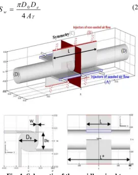
The tubular flame burner configurations considered in the present study (Fig. 1) are identical to the experimental configurations of Shi et al. (2014b). The burners are open on both sides. For the validation of the CFD code, two RTFB configurations were analyzed. The total length of burners is L* =10 D0 with D0 is the inner diameter which equals to 16 mm. The burners have four rectangular tangential injectors with a width W=0.125 D0 and a length L.

In order to validate our results and to analyze then the effect of number of injectors, five RTFB configurations were identified (Table 1). The swirl number S used to measure the swirl strength was defined by Beer and Chigier. (1972) as:





0 0

0 2 0

0 2

0/2) ( /2)

( R

R

x _{D ru dr}

dr uwr

D G

G

S  (1)

A D D S

T e w

4

0



 (2)

Fig. 1. Schematic of the rapidly mixed type tubular flame burner.

Where De is the exit throat diameter which defined by the following expression De=D0-W, AT=N*L*W is the total area of the tangential inlet injectors, N is the number of injectors and L is the injector length.

The two burner configurations studied as a validation of the CFD code are characterized by a geometrical swirl number (Sw) equal to 0.34 and 1.37 respectively (Table 1).

cTable 1Specifications of burner design

Table 1Specifications of burner design

Cases Number of Injectors, N

Area of the tangential inlet

slits, AT [m2_]

Geometrical swirl number,

Sw

Burner 1 4 512x10-6 _0.34

Burner 2 4 128 x10-6 _1.37

Burner 3 4 96 x10-6 _1.83

Burner 4 2 96 x10-6 _1.83

Burner 5 6 96 x10-6 _1.83

The mixing process was analysed by adopting the method proposed by Shi et al. (2013)-(2014a) (2014b) (2014c) based on the injection of Magnesium oxide particles (MgO) (Fig. 1). Indeed, for the burner with four injectors, seeded air (air + Magnesium oxide particles (MgO)) was introduced into the horizontal injectors (A), non seeded airflow was introduced into the other two injectors (B).

3. G

S

The computational domains of the different configurations were first generated and meshed by Gambit. The geometry of interest has a symmetrical nature. So, the simulative domain adopted here is the half of the tubular burner.

A hexahedral mesh with a structured boundary layer mesh near the burner wall was used since it is much more computationally efficient than the tetrahedral mesh. To reduce the total cell number and avoid a very large difference in cell volume between adjacent cells, the axial mesh distribution is increased progressively from the downstream slits to the outlet region.

In order to ensure the independence of the solution on the grid size, grid densities from 431 472 cells to 1 083 704 cells were tested for the computational domain. It was noticed that for a cells number varying between 879 040 to 1 083 704, the numerical results were similar. So, the choice of the grid size, which was based on the weakest computing time, was fixed to 879 040 cells (Fig. 2). The selected grid (879 040 cells) is locally refined in the near injection slits and boundary walls (Δy=Δz=3.10-4_{) as well as near the burner axis} (Δy=Δz=10-4_{) so as to predict more accurately the} trajectory of particles and the mixing process. Fig. 2 shows the overall grid structures adopted in this research.

Fig. 2.Grid system used in the computation.

4. N

M

A numerical investigation based on Reynolds-averaged Navier–Stokes (RANS) method is performed to examine the effect of number of injectors on the mixing process in Rapidly mixed type Tubular Flame Burner (RTFB).

The Eulerian–Lagrangian approach with a discrete phase method (DPM) was used to describe the solid particles motion in a flow field, i.e., the gas phase was considered as a continuum phase by solving Navier Stokes equations and the solid phase was calculated by tracking particles in the flow field.

4.1.

Assumptions

For all simulations, the following assumptions were considered:

- The flow is steady state and isothermal.

- The flow is laminar. Indeed, for all studied cases, the Reynolds number in the tube

“





0

Re  ” is less than the critical

Reynolds number of 300. (R.C. Chanaud 1963 and 1965).

- The particle phase is sufficiently diluted that particle-particle interactions

- The effects of the particle volume fraction on the gas phase are negligible.

- The volume fraction of discrete phase is less than 10–12% (Elghobashi 1994).

- The solid particles are spherical and non-deformable with a same diameter dp =10-6 m and density ρp =3580 kg/m3. Since the particle density is considerably larger than that of the fluid, i.e., ρp/ρ>>1, the Basset force, the buoyancy force, the virtual mass force and the pressure gradient force, could be neglected (D.E. Stock et al. (1996); Wenjing Sun et al. 2015).

4.2.

Governing Equations

Given the preceding assumptions, the governing equations can be written as follows:

0    x U i

i (3)





 (4)

The force balance on particles has been integrated to determine the trajectories of the solid particle (Fluent.2006). The particles motions are calculated with the following equation:





dU ₍₅₎

Where FD is the drag force per unit of mass and velocity difference (U-UP), U is the fluid phase velocity and UP is the particle velocity. FD is given by: 24 Re 18 2 p D p p D C d

F  



 (6)

μ is the molecular viscosity of the fluid, ρ is the fluid density, ρp is the density of particle, dp is the particle diameter, Rep is the relative Reynolds number of particles which is defined as





 U UP dp p

 

Re (7)

And CD is the drag coefficient given by:

2 3 2 1

Re

Rep p

D

a a a

C    (8)

Where the a’s are constants that apply for smooth spherical particles over several ranges of Rep given by S. A. Morsi and Alexander (1972).

The volume flow rate of the discrete phase

(Q N d uf

p p p 4 2 

 ) was chosen equal to 0.09

multiplied by the volume flow rate of the gas phase and the number of MgO particles introduced in the simulation at the corresponding inlets is respectively equal to 3584, 1260, 560, 560 and 560

for the burners 1, 2, 3, 4 and 5.

In this three-dimensional study, the MgO particles are considered to following exactly the flow, indeed for all treated cases the particles have a very small

Stokes number D u d N S f f p p p t 0 2    .

4.3.

Boundary Conditions and Solution

Strategies

The burners considered have four rectangular tangential injectors and two axial outlets. Since, the geometry of interest has a symmetrical nature. So, the simulative domain adopted here is the half of the RTFB. It means that the half of the total flow enters through the four tangential slots (with a length of L/2) and it comes out through a single axial outlet.

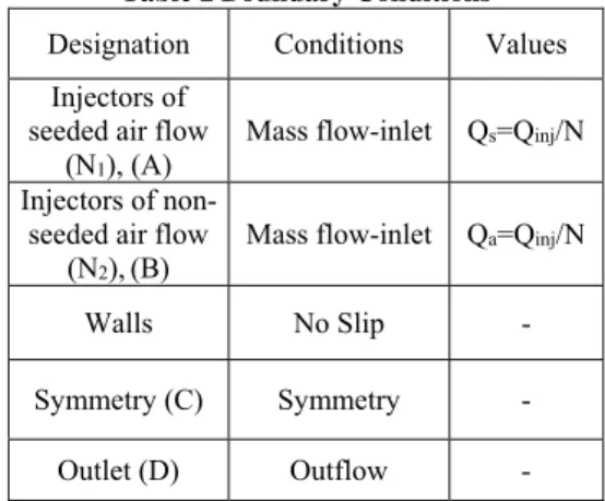
The boundary conditions illustrated in Fig. 1, are summarized in Table 2.

Table 2Boundary Conditions

Designation Conditions Values

Injectors of seeded air flow

(N1), (A)

Mass flow-inlet Qs=Qinj/N

Injectors of non-seeded air flow

(N2),(B)

Mass flow-inlet Qa=Qinj/N

Walls No Slip -

Symmetry (C) Symmetry -

Outlet (D) Outflow -

Numerical computations were carried out using Fluent which is based on the finite volume method. In order to improve accuracy, the second order upwind scheme was used. The SIMPLE method was applied to determine the pressure–velocity coupling. It uses a relationship between velocity and pressure corrections to enforce mass conservation and obtain the pressure field. The maximum residual of all variables was 10-4 _{in the} converged solution.

We noted that the N1 is the number of injectors type A which inject air/MgO and the N2 is the number of injectors type B which inject air.

5. R

A

D

5.1.

Validation of the Numerical Model

To give more confidence of the model, we established some quantitative and qualitative comparisons with the experimental data of Shi et al. (2014b).

(CRZ) and circumferential velocities results with the experimental results of Shi et al. (2014b).

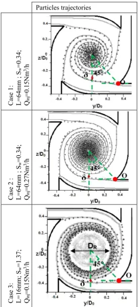
Three cases were considered:

- Case 1: L=64mm; Sw=0.34; Qinj=0.15Nm3/h;

- Case 2: L=64mm; Sw=0.34; Qinj =0.27Nm3/h;

- Case 3: L=16mm; Sw=1.37; Qinj =0.15Nm3/h.

The seeded air (air + MgO particles) is tangentially introduced into the burner by the two horizontal injectors. Or, non-seeded air was introduced by the other injectors. To simplify the flow visualization, the flow structure is determined by tracking the particles trajectories delimiting the flow injected through the horizontal slits.

Fig. 3. Predicted and experimental results of particle trajectories in a cross section for the three treated cases. + : Experimental data; Gray

line: Numerical results.

Figure 3 shows a confrontation between the predicted and experimental Shi et al. (2014b) results of flow structure for the three cases treated here. It is found that a satisfactory agreement with the experimental data (Shi et al. (2014b)) was obtained. Indeed, this method permits to describe

expansion (case 1 and 2) and shrinkage (case 3) of the jet thickness after being ejected outside the injector. Moreover, it is shown that the width of the air injected from the low side gradually shrinks with increasing the geometrical swirl number.

The dashed zone indicates surface contour of negative axial velocity which is used to identify the existence of the central recirculation zone (CRZ). This zone eventually appears only for the case 3 characterised by a geometrical swirl number larger than the critical swirl number (Sw>0.6). Indeed, Gupta et al. (1984) have established that the number of swirl must be higher than 0.6, value from which the flow develops recirculation zones.

The mixing layer thickness (δ) around the exit of the injector is defined as the width of the non seeded air flow from the upper right slit. This thickness was measured after an angle of 45 degrees of the starting point O (see Fig. 3) which is defined as the inner edge of the lower right injector.

Numerical and experimental results of the mixing layer thickness and the CRZ diameter are compared in Table 3. The discrepancy between these results is less than 5%. Thus, the obtained results agree well with those of Shi et al. (2014b).

Table 3Numerical and experimental mixing

layer thickness and CRZ diameter

Case 1

Case 2

Case 3

Ex. Nu. Ex. Nu. Ex. Nu.

δ

(mm) 1 1.05 0.8 0.84 0.75 0.79

DR

(mm) 0 0 0 0 8.51 8.59

0 0.1 0.2 0.3 0.4 0.5

r/D0 (m)

0 2 4 6

V/

Uav

(m

/s

)

Experiment of Shi et al. : Sw=0.34, Q=0.15 [Nm

3_/h]

Numerical: Sw=0.34, Q=0.15 [Nm3/h]

Experiment of Shi et al. : Sw=0.34, Q=0.27 [Nm3/h] Numerical: Sw=0.34, Q=0.27 [Nm3/h]

Experiment of Shi et al. :Sw=1.37, Q=0.15 [Nm

3_/h]

Numerical: Sw=1.37, Q=0.15 [Nm

3_/h]

Fig. 4. Numerical and experimental results of circumferential velocities at x/D0=0.

In Fig. 4, we compare numerical and experimental profiles of the tangential velocity at the injectors’ Particles trajectories

Case 1: L=64mm ; S

w

=0.34;

Qinj

=0.15Nm

3/h

Case 2 : L=64mm ; S

w

=0.34;

Qinj

=0.27Nm

3/h

Case 3: L=16mm; S

w

=1.37;

Qinj

=0.15Nm

outlet for the three treated cases. To analyse the statistical accuracy of the proposed model, the determination coefficient (R-square) and the P-value for the three cases have been calculated and presented in Table 4.

Table 4 Summary of R-square and P-value

Case 1 Case 2 Case 3

R-square 0.89 0.91 0.98

P-Value 10–7 ₁₀–7 ₁₀–8

As it can be seen on Table 4, the results are statistically significant with a high R-square (close to 1) and a low P-value (less than 10-7_{). So, the} agreement between the results is satisfactory which means that the adopted model offers a satisfactory prediction of the tangential velocity distributions.

This comparison proves the validity of our numerical model and justifies its use to discuss the effects of some parameters affecting the RTFB operating.

5.2.

Number of Injectors Effect

In this sub-section, we attempt to reveal the effect of number of injectors on the flow structure and the mixing process in a RTFB. The discussed results are thematically presented according to the following subtopics: “flow structure (particle trajectories and CRZ)”, “local swirl intensity” and “Mixing layer thickness”.

Three burner configurations with different number of injectors (N=2, 4, 6) have been considered (Table 1).

5.2.1.

Flow Structure

The total flow rate is fixed at a value of 410-5 _Kg s-1_{, i.e. almost the same Reynolds number (Re}

T). It should be noted also that all the tested burners have the same geometrical swirl number (Sw=1.83).

In Fig. 5, the particle trajectories in the cross section perpendicular to the tube axis (x=0, y, z) for different numbers of injectors were presented. For all the tested burners, it is shown that the flow width shrinks after being ejected outside the injector generating a very intense centrifugal force. This strong centrifugal force causes the pressure drop in the center causing the appearance of a central recirculation zone.

Moreover, the mixing layer thickness ‘previously defined” seems to be constant for the three burners. However, this is only true for a general observation. In reality, an important decrease of the mixing coefficient is visible, especially between burner 4 and burner 5. This result is discussed with more details in the section of the mixing layer thickness. Moreover, it is noted that the seeded air width after injection decreases and the diameter of CRZ increases by increasing the number of injectors, which according to B.shi et al. (2014b), results in the decrease the mixing time in the burner (Eqs. (10) and (11)).

Burner 3

Burner 4

Burner 5

Fig. 5. Particles trajectories in a cross section varying with number of injectors.

These observations lead to conclude that for the same geometrical swirl (Sw) and Reynolds (ReT) numbers, the increase of the number of injectors promotes the mixing process in rapidly tubular flame burner.

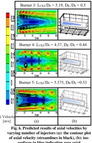
The Fig. 6 illustrated, at the left side, the contour plot of axial velocity and streamlines on the plane (x, y, z=0m) and the iso-surfaces (U=0) indicating central recirculation zones at the right side for burner 3, 4, 5 respectively.

The streamlines present a radial vortex bubble shift towards the inlet plane with increasing the number of injectors. This vortex manifests on the periphery of the central recirculation zone (CRZ). This zone is located in the central region. It has the same conical form for the three burners. This happens due to the decrease of the swirl motion while going downstream of the swirl generating device, decreasing thus the centrifugal force and consequently the adverse pressure gradient. The size of the CRZ becomes more extended with increased number of injectors (seen Fig. 6). This happens due to the inlet mass flow distribution effect.

Burner 3: LCRZ/D0 = 5.19, DR /D0 = 0.5

Burner 4: LCRZ/D0 = 4.37, DR /D0 = 0.44

Burner 5: LCRZ/D0 = 5.375, DR/D0 =0.53

(a) (b)

Fig. 6. Predicted results of axial velocities by varying number of injectors (a): the contour plot

of axial velocity (streamlines in black), (b): iso-surfaces in blue indicating zero axial

velocity (U=0) zones.

5.2.2.

Local Swirl Intensity

In this subsection, the total flow rate and the geometrical swirl number are fixed at a value of 410-5 _{Kg s}-1 _{and 1.83, respectively.}

For design purposes, it is major to understand the swirl decay process along the burner. The Swirling motion decay is an inevitable effect in swirl flows resulting from shear stresses. To calculate Swirl decay, it is suitable to calculate the swirl number along the burner axis using Eq. (1).

Fig. 7. Swirl intensity distributions for various number of injectors along the pipe axis.

Figure 7 depicts the local swirl intensity distribution along the burner axis for different number of injectors. According to Hay and West (1975), F. Chang and V. K. Dhir (1994) and Steenbergen and Voskamp (1998), local swirl number with an exponential manner except for axial distances less than two diameters downstream the inlet. The local

swirl decrease can be approximated as exponential function (S=A exp (B* x/D0); where A and B are depending to the geometrical swirl number and the number of injectors).

Fig. 8. Variations of Ln(S/S N ))/(N S0.22))

w 0.2 0.62 0.78 w according to (x/D0).

In the Fig. 8, Ln(S/Sw0.78N0.62))/(N0.2Sw0.22))is presented as a function of (x/D0). As you can see in the Fig. 8, the three curves of Fig. 7 are transformed into a single linear line passing through the origin with a slope of -0.15.

So, the local swirl number can be correlated in terms of geometric swirl number and number of injectors as follows:

) 15

. 0 exp(

0 22 . 0 2 . 0 62

. 0 78 . 0

D x S N N

S

S w  w (x/D0≥2) (9)

5.2.3.

Mixing Layer Thickness

The effect of the number of injectors on the mixing time was examined. To quantify this effect, the mixing coefficient K is also determined. Indeed, the coefficient K is an essential parameter in determining the Damkhöler number (Da= τm / τr) where τm is the mixing time that is expressed based on K as follows:

D V

K

mass inj m

2



 (10)

Where Dmass is the mass diffusivity. The mixing coefficient K was determined according to the work of Shi et al. (2013, 2014a, 2014b, 2014c) who have found that the flow near the slits is dominated by a boundary layer type flow. So, they were demonstrated that the mixing layer thickness (δ) determined after 45 degrees from the starting point O (see Fig. 3) can be expressed as a function of injection velocity, as follows:

V K

inj



 (11)

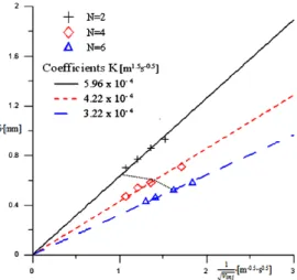
In this subsection, the injection velocity was varied for the three burners (burner 3, 4 and 5). The corresponding width  is plotted as a function of

Vinj

1

(see Fig. 9). It is shown that the flow

around the exit of the injector is dominated by a X Velocity

boundary layer type flow (Shi et al. (2014a) (2014b) (2014c)). At a constant total flow rate (QTotal) shown by the dotted line, it has been noted the width  gradually decreases with increasing the number of injectors.

Fig. 9. Boundary layer type flow around the exit of injector varying with the number of injectors.

For fixed injection velocity Vinj=1 m/s, it is shown that the mixing layer thickness reaches its maximum for the case with low number of injectors (N=2) (corresponding to the smaller values of total flow rate, QTotal=N* Q). Indeed, the burner 4 (N=2) gives the upper limit of mixing coefficient (K=5.9610-4 _m1.5 _s-0.5_{). By gradually increasing the} number of injectors, i.e. the total flow rate increases, resulting in the decrease of the mixing coefficient. According to these observations and Eqs. (10) and (11), we can conclude that the burner with higher number of injectors ensures a better mixing time.

6. C

In this paper, a numerical investigation based on Reynolds-averaged Navier–Stokes (RANS) method is performed to examine the effect of number of injectors on the mixing process in Rapidly mixed type Tubular Flame Burner (RTFB). To analyse the non reactive mixing process, the method adopted by Shi et al. (2014b) based on the injection of Magnesium oxide particles (MgO) is used (Fig. 1).

Numerical simulations were performed using Fluent 6.3 which is based on the finite volume method. Solid particles motion in a flow field were described by the Eulerian–Lagrangian approach with a discrete phase method (DPM), i.e., the gas phase was treated as a continuum by solving Navier Stokes equations and the solid phase was calculated by tracking particles in the Flow field.

We started our results by comparing the numerical results to the experimental data of Shi et al. (2014b) in order to validate our numerical model. The results of the flow structure, mixing layer thickness, diameter of the central recirculation zone (CRZ) and circumferential velocities were compared and a

good agreement was found. Thereafter, we analysed the mixing process for different numbers of injectors and we noticed that, for the same geometrical swirl (Sw) and Reynolds (ReT) numbers, the air width after injection decreases and the diameter of CRZ increases with the increase of the number of injectors. This happens due to the increase of the swirl number near the inlet, increasing thus the centrifugal force and consequently the adverse pressure gradient. Thus, the increase of number of injectors promotes the mixing process in rapidly tubular flame burner. On the other hand, we correlated the swirl decay along of the RTFB in terms of geometric swirl number and number of injectors and we determined the mixing coefficient for each burner.

R

Alekseenko, S. V., P. A. Kuibin, V. L. Okulov and S. I. Shtork (1999). Helical vortices in swirl flow. Journal of Fluid Mechanics 382, 195-243.

Avci, A., I. Karagoz, A. Surmen and I. Camuz (2013). Experimental Investigation of the Natural Vortex Length in Tangential Inlet Cyclones. Separation Science and Technology (Philadelphia) 48(1), 122-126

Azim, M. A. (2016). Mixing of Co-Axial Streams: Effects of Operating Conditions. Journal of Applied Fluid Mechanics 9(2), 751-756.

Beer J. M. and N. A. Chigier (1972). Combustion Aerodynamics. Applied Science Publishers I., 100-117.

Cakmak, G., Z. Argunhan and C. Yildiz (2011). Effect of swirl generators with different sized propeller on heat transfer enhancement. Energy Education Science and Technology Part A: Energy Science and Research 27(2), 323-330

Chanaud, R. C. (1963). Experiment concerning the vortex whistle. J. Acoust. Soc. Am. 35(7), 953-960.

Chanaud, R. C. (1965). Observations of oscillatory motion in certain swirling flows. J. Fluid Mech. 27, 11-21.

Chang, F. and V. K. Dhir (1994). Turbulent flow field in tangentially injected swirl flows in tubes. International Journal of Heat and Fluid Flow 15, 346-356.

Elghobashi, S. (1994). On predicting particle-laden turbulent flows. Appl. Sci. Res. 52, 309-329.

Fluent (2006). FLUENT 6.3user’s guide.

Guizani, R., I. Mokni, H. Mhiri and P. Bournot (2014). CFD modeling and analysis of the fish-hook effect on the rotor separator's efficiency. Powder Technology 264, 149-157.

Hay, N. and P. D. West (1975). Heat transfer in free swirling flow in a pipe. Journal of Heat Transfer 97, 411-417.

Ishizuka, S., T. Motodama and D. Shimokuri (2007). Rapidly mixed combustion in a tubular flame burner. Proc. Combust. Inst. 31, 1085-1092.

Khaldi, N., Y. Chouari, H. Mhiri and P. Bournot (2016). CFD investigation on the flow and combustion in a 300 MWe tangentially fired

pulverized-coal furnace. Heat and Mass

Transfer 9(5), 2359-2367.

Kitoh, O. (1991). Experimental study of turbulent swirling flow in a straight pipe. Journal of Fluid Mechanics 225, 445-479.

Klančišar, M., T. Schloen, M. Hriberšek and N. Samec (2016). Analysis of the Effect of the Swirl Flow Intensity on Combustion Characteristics in Liquid Fuel Powered Confined Swirling Flames. Journal of Applied Fluid Mechanics 9(5), 2359-2367.

Mantilla, I. (1998). Bubble Trajectory Analysis in Gas–Liquid Cylindrical Cyclone Separators. Master’s thesis, The University of Tulsa.

Martemaniov, S. and V. Okulov (2004). On heat transfer enhancement in swirl pipe flows. International Journal of Heat and Mass Transfer 47, 2379-2393.

Morsi, S. A. and A. J. Alexander (1972). An Investigation of Particle Trajectories in Two-Phase Flow Systems. J. Fluid Mech. 55(2), 193-208.

Pathak, M., Dewan A. and A. K. Dass (2005). An assessment of streamline curvature effects on the mixing region of a turbulent plane jet in crossflow. Applied Mathematical Modelling 29, 711-725.

Ranga Dinesh K. K. J., M. P. Kirkpatrick and K. W. Jenkins (2010). Investigation of the influence of swirl on a confined coannular swirl jet. Computers and Fluids 39, 756-767.

Shi, B., D. Shimokuri and S. Ishizuka (2013). Methane/oxygen combustion in a rapidly

mixed type tubular flame burner. Proc. Combust. Inst. 34, 3369-3377.

Shi, B., D. Shimokuri and S. Ishizuka (2014a). Reexamination on methane/oxygen combustion in a rapidly mixed type tubular flame burner. Combust. Flame 161, 1310-1325.

Shi, B., J. Hu and S. Ishizuka (2014c). Carbon dioxide diluted methane/oxygen combustion in a rapidly mixed tubular flame burner. Combust. Flame 162, 420-430.

Shi, B., J. Hu, H. Peng and S. Ishizuka (2014b). Flow visualization and mixing in a rapidly mixed type tubular flame burner. Experimental Thermal and Fluid Science 54, 1-11.

Steenbergen, W. and J. Voskamp (1998). The rate of decay of swirl in turbulent pipe flow. Flow Measurement and Instrumentation 9, 67-78.

Stock, D. E. (1996). Particle dispersion in flowing gases, Freeman Scholar Lecture. J. Fluids Eng. 118, 4-17.

Sun, W., W. Zhong and Y. Zhang (2015). LES-DPM simulation of turbulent gas-particle flow on opposed round jets. Powder Technology 270, 302-311.

Syred, N. and J. M. Beer (1974). Combustion in swirling flows: a review. Combust. Flame 23, 143-201.

Tatsumi, K., M. Tanaka, P. Woodfield and K. Nakabe (2010). Swirl and buoyancy effects on mixing performance of baffle-plate-type miniature confined multijet. International Journal of Heat and Fluid Flow 31, 45-56.

Vahidifar, S. and M. Kahrom (2015). Experimental study of heat transfer enhancement in a heated tube caused by wire-coil and rings. Journal of Applied Fluid Mechanics 8(4), 885-892