www.nat-hazards-earth-syst-sci.net/12/187/2012/ doi:10.5194/nhess-12-187-2012
© Author(s) 2012. CC Attribution 3.0 License.
and Earth
System Sciences
Physically-based modelling of granular flows with Open Source GIS
M. Mergili1, K. Schratz2, A. Ostermann2, and W. Fellin3
1Institute of Applied Geology, BOKU University of Natural Resources and Life Sciences Vienna, Peter-Jordan-Straße 70, 1190 Vienna, Austria
2Department of Mathematics, University of Innsbruck, Technikerstraße 13, 6020 Innsbruck, Austria
3Unit of Geotechnical and Tunnel Engineering, University of Innsbruck, Technikerstraße 13, 6020 Innsbruck, Austria Correspondence to:M. Mergili ([email protected])
Received: 29 April 2011 – Revised: 28 October 2011 – Accepted: 4 December 2011 – Published: 17 January 2012
Abstract. Computer models, in combination with Geo-graphic Information Sciences (GIS), play an important role in up-to-date studies of travel distance, impact area, velocity or energy of granular flows (e.g. snow or rock avalanches, flows of debris or mud). Simple empirical-statistical rela-tionships or mass point models are frequently applied in GIS-based modelling environments. However, they are only ap-propriate for rough overviews at the regional scale. In detail, granular flows are highly complex processes and physically-based, distributed models are required for detailed studies of travel distance, velocity, and energy of such phenomena. One of the most advanced theories for understanding and mod-elling granular flows is the Savage-Hutter type model, a sys-tem of differential equations based on the conservation of mass and momentum. The equations have been solved for a number of idealized topographies, but only few attempts to find a solution for arbitrary topography or to integrate the model with GIS are known up to now. The work presented is understood as an initiative to integrate a fully physically-based model for the motion of granular flows, physically-based on the extended Savage-Hutter theory, with GRASS, an Open Source GIS software package. The potentials of the model are highlighted, employing the Val Pola Rock Avalanche (Northern Italy, 1987) as the test event, and the limitations as well as the most urging needs for further research are dis-cussed.
1 Introduction
Granular flows – including avalanches of snow, mud, debris or even rocks – are highly destructive phenomena putting people, buildings and infrastructures at risk. Delineation of possible impact areas as well as flow velocities is an essen-tial precondition for efficient action towards risk reduction,
e.g. designation of hazard zones for land use planning, di-mensioning of technical structures etc. (Hungr et al., 2005; Pudasaini and Hutter, 2007).
Since the 1990s, Geographic Information Sciences (GIS) have played an increasing role in the mapping and predic-tion of landslide, debris flow, and avalanche hazard and risk. They enable an efficient management of spatial data at all scales, usually in raster or vector format.
On a regional or even national level, GIS have a high popularity for identifying areas with high landslide hazard and risk and for generating so-called landslide susceptibil-ity maps. A large array of statistical methods has been ap-plied for this purpose (e.g. Corominas et al., 2003; Lee, 2004; Guzzetti et al., 2006). Also regarding physically-based methods, which require more detailed topographic and geotechnical information and are therefore mainly applicable at the small catchment scale, various approaches have been worked out and several GIS-based studies on shallow slope failures have been published (e.g. Godt et al., 2008). Pro-grams likeSINMAP(Pack et al., 1998) orSHALSTAB (Di-etrich and Montgomery, 1998) work as extensions to pro-prietary GIS software packages. Mergili and Fellin (2011) implemented a model for rotational failures with the Open Source package GRASS GIS(GRASS Development Team, 2011). However, GIS-based model development has focused to a lesser extent on the movement itself, but rather on the onset of the movement.
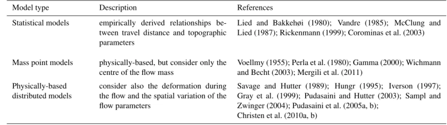
Table 1.Types of models for granular flows, partly based on Pudasaini and Hutter (2007).
Model type Description References
Statistical models empirically derived relationships be-tween travel distance and topographic parameters
Lied and Bakkehøi (1980); Vandre (1985); McClung and Lied (1987); Rickenmann (1999); Corominas et al. (2003)
Mass point models physically-based, but consider only the centre of the flow mass
Voellmy (1955); Perla et al. (1980); Gamma (2000); Wichmann and Becht (2003); Mergili et al. (2011)
Physically-based distributed models
consider also the deformation during the flow and the spatial variation of the flow parameters
Savage and Hutter (1989); Hungr (1995); Iverson (1997); Gray et al. (1999); Pudasaini and Hutter (2003); Sampl and Zwinger (2004); Pudasaini et al. (2005a, b);
Christen et al. (2010a, b)
Statistical models are employed for the estimation of key parameters (particularly travel distance). Threshold values of slope angles or horizontal and vertical distances (e.g. Lied and Bakkehøi, 1980; McClung and Lied, 1987; Bur-ton and Bathurst, 1998 based on Vandre, 1985; Coromi-nas et al., 2003), related to volume (e.g. Rickenmann, 1999; Scheidl and Rickenmann, 2009 for debris flows) are used as criteria. Such relationships are gained from the analysis of historical events. Some approaches also include basic physi-cal principles (Blahut et al., 2010; Kappes et al., 2011). Sta-tistical models are used today in combination with GIS and are often applied for regional-scale studies (e.g. Mergili and Schneider, 2011 for glacial lake outburst floods).
Mass point models (sometimes referred to as semi-deterministic or conceptual models) for snow avalanches or debris flows go back to the work of Voellmy (1955), who related the shear traction at the base to the square of the velocity and assumed an additional Coulomb friction ef-fect (Pudasaini and Hutter, 2007). This approach consid-ers only the centre of the flowing mass but not its defor-mation and the spatial distribution of the flow parameters. The Voellmy (1955) model was further developed and ap-plied e.g. by Perla et al. (1980); Gamma (2000); Wich-mann and Becht (2003); and Mergili et al. (2011). With statistical and mass point models, random walk procedures based on Monte Carlo techniques (Gamma, 2000) are used for routing the flow. As Van Westen et al. (2005) showed, the influence of the routing algorithm on the modelled areas of deposition is considerable.
Physically-based distributed models require more special-ized input information and are therefore suitable for local-scale studies. Movements are computed based on physical laws, assuming specific flow rheologies (Savage and Hut-ter, 1989; Takahashi et al., 1992; Hungr, 1995; Iverson, 1997; Pudasaini and Hutter, 2003; McDougall and Hungr, 2004, 2005; Pudasaini et al., 2005a, b). GIS applications of such models are still rather scarce. Some examples ex-ist where numerical models can be coupled with propri-etary GIS software, e.g.FLO-2D(O’Brien, 2003),SAMOS
(Sampl and Zwinger, 2004) or an application of the Taka-hashi et al. (1992) model (Chau and Lo, 2004). Some other models have been used in combination with GRASS GIS, likeDAN(Hungr, 1995; Revellino et al., 2008) or TI-TAN2D(Pitman et al., 2003). TheRAMMSmodel (Chris-ten et al., 2010a, b), primarily applied to snow avalanches, uses Voellmy (1955) viscous drag and runs with GRASS GIS in the background. However, a full GIS implementa-tion of more complex models (e.g. Savage and Hutter, 1989; Iverson 1997; Pudasaini and Hutter, 2003; see Pudasaini and Hutter, 2007 for a comprehensive list of references) still re-mains a challenge. Recently, there has been rapid progress in theoretical modelling, numerical simulation and valida-tion of the models with experimental and field data for gran-ular flows (Gray et al., 1999; Pudasaini et al., 2005a; Pu-dasaini et al., 2008; Luca et al., 2009a, b, c, d; PuPu-dasaini, 2011b). Zwinger et al. (2003) adapted the Savage-Hutter model for arbitrarily shaped mountain terrain, introducing some geometric simplifications. Based on Nessyahu and Tadmor (1990) and Tai et al. (2002), Wang et al. (2004) devised a numerical scheme applicable to flows over com-plex shallow terrain along a horizontally straight flow path (Gray et al., 1999). Pudasaini and Hutter (2003) proposed an avalanche model for generally curved and twisted chan-nels which was further developed by Pudasaini et al. (2005a, b, 2008). The simulation results were verified with experi-mental data. The Gray et al. (1999) and the Pudasaini and Hutter (2003) model are both based on curvilinear coordi-nate systems. Whilst such general models are adequate for the problems related to arbitrarily shaped mountain terrain, substantial efforts are still needed to apply these equations to real-world mountain topographies in connection with con-ventional raster-based GIS environments. This requires some adaptations which will be explained later.
distribution and evaluation: the program code is freely acces-sible and new modules may be added by anybody. Therefore, the entire scientific community has the chance to contribute to the evaluation of the model and the further development of the program code. Examples of GRASS implementations of mass movement models are provided e.g. by Cannata and Molinari (2008) and Mergili et al. (2011).
The GRASS module developed was namedr.avalanche. It builds on a numerical scheme devised by Gray et al. (1999), Pudasaini (2003), and Wang et al. (2004) for simple concave topographies with an only vertically curved flow line (Fig. 1). Pudasaini et al. (2005a, b, 2008) further applied these numer-ical schemes to more complex curved and twisted topogra-phies, and compared the model simulations with laboratory and field data for dry avalanches and mixture debris flows. Future work should be directed towards extending the scope of the physical and numerical model to arbitrary mountain terrain.
2 Methods
2.1 Model basics
The extended Savage-Hutter Model (Savage and Hutter, 1989; Gray et al., 1999; Pudasaini and Hutter, 2003) is ex-pressed as a system of partial differential equations describ-ing the conservation of mass and momentum for the rapid motion of dry granular avalanches:
∂h ∂t +
∂ ∂x(hu)+
∂
∂y(hv)=0, (1)
∂ ∂t(hu)+
∂ ∂x
hu2+ ∂
∂y(huv)=hsx− ∂ ∂x
βxh2
2 !
, (2)
∂ ∂t(hv)+
∂
∂x(huv)+ ∂ ∂y
hv2=hsy− ∂ ∂y
βyh2
2 !
, (3)
wherehis the avalanche thickness, anduandvare the depth-averaged downslope and cross-slope velocities.sxandsyare
the net driving accelerations:
sx=sinζ−√ u
u2+v2tanδ(cosζ+λκu 2)
−εcosζ∂b ∂x, (4) sy= −
u
√
u2+v2tanδ(cosζ+λκu 2)
−εcosζ∂b
∂y, (5)
whereζ is the downslope inclination angle of the reference surface,κ is the local curvature of the reference surface,b
is the elevation above the reference surface, andεandλare some scaling factors (see Sect. 2.3.2).βxandβyare defined as
βx=εcosζ Kx, (6)
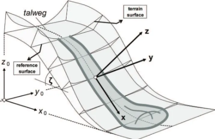
Fig. 1. Idealized topography for the solution of the extended Savage-Hutter Model by Wang et al. (2004), also used for
r.avalanche.
βy=εcosζ Ky. (7)
KxandKy are the earth pressure coefficients in downslope and cross-slope directions (as computed at the basal surface):
Kx,act/pass=2 1∓ r
1−cos2φ.cos2δ !
sec2φ−1, (8)
Ky,act/pass= 1 2
Kx+1∓ q
(Kx−1)2+4tan2δ
. (9)
φis the angle of internal friction, andδis the bed friction an-gle. Active stress rates (subscript act) are connected to local elongation of the flowing mass, passive stress rates (subscript pass) are connected to local compacting – it depends on ac-celeration or deac-celeration of the flow whether active or pas-sive stress rates are applied (Gray et al., 1999). The system of equations described above is only valid for the shallow flow of cohesionless and incompressible granular materials which can be considered as continuum. The model is often applied to cases with non-shallow onset areas. This is acceptable as long as the movement quickly transforms into a shallow flow, since the geometry during the flow and the deposition does not much depend on the geometry of the onset mass in such cases. The curvature of the terrain has to be relatively small. It has to be emphasized that all variables are dimensionless. The model is scale-invariant and small-scale laboratory tests can be used as reference for large-scale problems in nature. 2.2 Numerical solution of the equations
The differential equations Eqs. (1) to (3) were solved us-ing a high resolution Total Variation Diminishus-ing Non-Oscillatory Central Differencing (TVD-NOC) Scheme, a nu-merical scheme useful to avoid unphysical nunu-merical oscil-lations (Nessyahu and Tadmor, 1990). Cell averages ofh,
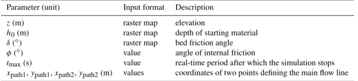
Table 2. Input parameters forr.avalanche.
Parameter (unit) Input format Description
z(m) raster map elevation
h0(m) raster map depth of starting material δ(◦) raster map bed friction angle φ(◦) value angle of internal friction
tmax(s) value real-time period after which the simulation stops xpath1,ypath1,xpath2,ypath2(m) values coordinates of two points defining the main flow line
is moved half of the cell size with every time step, the val-ues at the corners of the cells and in the middle of the cells are computed alternatively. The TVD-NOC scheme with the minmod limiter has been successfully applied to a large num-ber of avalanche and debris flow problems (Tai et al., 2002; Wang et al., 2004; Pudasaini et al., 2005a, b, 2008, Pudasaini and Kroener, 2008). Here, this scheme is implemented in the r.avalanchecomputational tool.
The simulation is run for a user-defined, real-time period; in the future it is planned to implement a criterion based on the absolute value of the average velocity of the flow, with a user-defined sufficiently low threshold value. The time steps have to be kept short enough to fulfil the Courant-Friedrichs-Levy (CFL) condition:
1t
1x|cmax|<
1
2, (10)
cmax= max alli,j
ui,j +
p
βxhi,j,vi,j +
p
βyhi,j, (11)
where1x is the cell size inx direction,cmaxis the global maximum wave speed andiandj are the coordinates of the cells inx andy direction, respectively. 1t is determined dynamically during the run-time ofr.avalanche, based on the CFL condition from the previous time step.
2.3 Implementation into GRASS GIS
2.3.1 Layout
r.avalanche was developed as a raster module for GRASS GIS, using the C programming language. Raster maps and a set of parameters compiled in a text file serve as input (see Table 2). The implementation of the model and the numerical scheme described above into GIS should consider the following:
– Eqs. (1) to (3) provide dimensionless values. However, in real flow simulations, for better physical intuition, it is desirable to use dimensional values;
– in general the solution is obtained for a curvilinear ref-erence system. However, this must be converted into a rectangular GIS system.
In reality the avalanche valleys are not only curved in the downslope direction, but also in the cross-slope direction. Here, for simplicity, the idealized situation that the slope is only curved in the downslope direction but laterally flat is assumed (Gray et al., 1999). However, as in Puda-saini et al. (2005a, b, 2008), it would be more realistic to construct the mountain topography based on a curved and twisted surface or even better, on arbitrary topography. This could be an interesting future direction, but is not within the scope of this paper.
2.3.2 Non-dimensionalization of the variables
The first issue concerns the non-dimensionalization of the governing variables and parameters, which is explained e.g. in Pudasaini (2003). With the typical avalanche lengthL, the typical avalanche depthHand the typical radius of curvature
R, the dimensional variables are derived by using ⌢
x,⌢y=(Lx,Ly) ⌢
h,⌢b=(H h,H b) ⌢
u,⌢v= u√gL,v√gL ⌢
t =t q
Lg ⌢
κ=κR
, (12)
where the variables denoted with a cap are the dimensional counterparts of the variables used in Eqs. (1) to (3) and g
is gravitational acceleration. The implemented model com-putes the dimensionless variables and converts them to di-mensional values according to Eq. (12) for output. The scal-ing parametersL,H, andR are set to 1 in this paper. The factorsε=H/Landλ=L/R(Pudasaini, 2003) are therefore 1 as well. However, the choice of the scaling parameters does not influence the numerical results since Eqs. (1) to (9) are scale invariant.
2.3.3 Adaptation of the coordinate system
1
Fig. 2.Iterative determination ofbbased on the coordinate system defined by the reference plane.
Here, as in Gray et al. (1999) and Wang et al. (2004), it is assumed that the talweg is only curved in the downslope di-rection so that its projection to a horizontal plane is a straight line (see Fig. 1). Three steps are required for converting the original rectangular coordinate system of the input raster maps into the coordinate system for the simulation:
– the coordinate system is rotated around thez axis so that the direction of the main flow line is aligned with the newx (downslope) direction. The main flow line is based on two user-defined pairs of coordinates (see Table 2);
– a reference surface is created, defined by the given tal-wegand an inclination of zero iny (cross-slope) direc-tion. As the talweg follows the natural terrain, its lon-gitudinal section (Fig. 2) does not represent a straight or regularly curved line like in the idealized topography shown in Fig. 1;
– based on this reference surface, the cell size1xfor each
x parallel to the reference surface is computed. The offsetb (m) – defined as the distance between terrain surface and reference surface perpendicular to the ref-erence surface – is derived. Since the terrain surface is not given analytically andz0,terrainin Fig. 2 depends on the correspondingx0,b has to be determined itera-tively. This is done by varying the horizontal shift until the tested value ofz0,testconverges to the terrain surface. The terrain height is interpolated between the centres of the two closest raster cells in the direction ofx0. Initial avalanche thicknessh is derived in an analogous way. As a final step, all raster maps are resampled in order to set1x=1y=const. (a precondition for applying the numerical scheme used by Wang et al., 2004).
After completing the simulation, the entire system is re-converted into the rectangular coordinate system used in the
1
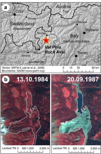
Fig. 3. Val Pola Rock Avalanche:(a)location;(b)comparison of Landsat imagery before and after the event.
GRASS GIS mapset in order to enable a proper display of the results.
3 Study area and data
3.1 The 1987 Val Pola Rock Avalanche
debris flows were reported from the tributaries to the Valtel-lina. The Val Pola Creek was deeply eroded, undercutting the northern edge of an old landslide body. Preceded by the opening of a prominent crack, a block of highly fractured and faulted igneous and metamorphic rocks detached and rushed into the valley (Crosta et al., 2003). Figure 3b provides a comparison of satellite views of the area before and after the event.
The volume of the released mass was estimated to 34– 43 million m3 (Crosta et al., 2003) and 35 million m3 (Govi et al., 2002), the entrainment by the resulting rock avalanche to further 5–8 million m3. After detaching, the mass first moved northwards until rushing against the Sassavin-Motta Ridge, and then proceeded as rock avalanche eastwards down to the main valley. Govi et al. (2002) dis-tinguished six phases of the movement, with a duration of the main avalanching phase of 8–12.5 s. The velocity of the flow was estimated to peak at 76–108 m s−1 (Crosta et al., 2004), indicating that the event was one of the most rapid documented mass movements in history.
The mass moved up 300 m on the opposite slope. In the main valley, it continued 1.5 km downstream and 1.5 km up-stream, with a maximum thickness of 90 m (Crosta et al., 2003; see Fig. 3b). The Adda river was dammed, and a lake started to form, the level rising several metres per day. An artificial drainage was constructed rapidly in order to avoid an uncontrolled sudden drainage of the lake. The event claimed 27 human lives and caused high economic costs (Crosta et al., 2003).
3.2 Data
The following data sets were obtained for the Val Pola Rock Avalanche:
– Digital Elevation Models (DEMs) before and after the event;
– geotechnical parameters of the sliding mass and the slid-ing surface;
– reference information on the distribution of the deposit. A DEM provided by the Geoportal of the Region Lombardy (Italy; www.cartografia.regione.lombardia.it) at a cell size of 20 m was used. It represents the situation before the 1987 Val Pola event. An SRTM-4 DEM (Jarvis et al., 2008) from February 2000 was obtained in order to capture the situation after the event. It has a cell size of 3 arc seconds and was resampled to 20 m, too. However, it was mainly used for defining the depth of the failure plane whilst the pre-failure DEM was applied for the simulation.
The distribution of the released mass was estimated from the difference between the two DEMs. A volume of ap-prox. 40 million m3was derived, being well within the range reported by Crosta et al. (2003, 2004). The higher value
Fig. 4. Val Pola Rock Avalanche. Distribution of detached and deposited volumes as derived from the DEM change detection, the flow trimline was mapped from Landsat TM imagery (thick black line).
compared to that one reported by Govi et al. (2002) can be explained by the fact that material detached from the Sassavin-Motta Ridge – considered as entrained material by those authors – is included here (Fig. 4). Furthermore, the de-fined onset area is larger than shown by Crosta et al. (2003). This counterbalances the fact that entrainment is disregarded byr.avalanche. In general, it is hard to clearly delineate the zones of onset and entrainment by the mass flow. The accu-racy of the DEMs did not allow for a reliable estimate of entrained and deposited volume. However, the maximum thickness of deposited material derived by the DEM over-lay was 83 m and therefore close to the value reported by Crosta et al. (2003) and Govi et al. (2002). However, this overlay has to be considered as a rough approximation since significant anthropogenic reshaping of the terrain took place after the event. Only areas with a derived thickness of the deposit≥20 m are shown in Fig. 4. The affected area as ref-erence data was mapped from Landsat TM imagery and veri-fied with the Italian Landslide Inventory (IFFI Project) and a map published by Crosta et al. (2003). Possible inaccuracies are caused by secondary processes, e.g. mud flows down-stream blurring the delineation of the impact area downval-ley.
Table 3.Parameter combinations applied for the simulations.
cell size δ φ talweg (m) (◦) (◦) assumption Simulation 01 20 22 35 1 Simulation 02 40 22 35 1 Simulation 03 12 22 35 1 Simulation 04 20 22 35 2 Simulation 05 20 18 35 1 Simulation 06 20 26 35 1 Simulation 07 20 22 40 1 Simulation 08 20 22 45 1
a Drucker-Prager model, whilst the Savage-Hutter Model is based on a Mohr-Coulomb model. Therefore, and since Crosta et al. (2003) used a two dimensional model with plane strain condition, these values are not directly applicable to the present study. Crosta et al. (2004) back-calculated the event in a three-dimensional way with a Lagrangian Finite Element Model (LFEM), assuming a basal friction angle of 22◦and a dynamic internal friction angle of 35◦. These val-ues were used as a base also for the present study. How-ever, it has to be emphasized that the parameters were not directly derived from laboratory tests but indirectly by fitting the model results to the observations.
The standard cell size for the computation was set to 20 m, according to the DEM used. The model was also tested with 40 m and 12 m cell size, respectively. Furthermore, two dif-ferent assumptions of the talweg (see Fig. 4) were tested: talweg 1 starting farther N than the centre of the affected area (accounting for the fact that the detached mass moved northwards before converting into a rock avalanche), and talweg 2 along the centre of the affected area. All simula-tions were run for a real-time duration of 300 s, following Crosta et al. (2004) and the observation that no substantial temporal changes of the height and geometry of the modelled deposit were observed at that time.
The single-phase model used does not allow for consider-ing landslide-river interactions that may have occurred when the rock avalanche plunged into the Adda river. However, future model development will go in this direction (see Con-clusions).
4 Results
4.1 Test with simple artificial topography
Before being applied to the Val Pola Rock Avalanche, r.avalanchewas tested for a simple plane slope with an incli-nation of 35◦, running out into a horizontal plane. Assuming a hemispherical starting mass, the simulation was run with four combinations ofφ(30◦ and 37◦) and δ(23◦ and 28◦). The model responded much less sensitively to variations of
Fig. 5. Granular flow over an inclined surface running out into a horizontal plane withφ=30◦andδ=23◦and 28◦, respectively:
(a)longitudinal profiles, flow depth 15-fold exaggerated compared to terrain height;(b)flow depth maps (colours forδ=28◦and con-tour lines forδ=23◦). The shorter travel distance withδ=28◦is obvious.
φthan to variations ofδ. Maps and longitudinal sections il-lustrating the results forφ=30◦are shown in Fig. 5. The patterns yielded byr.avalanchecorrespond well to those pre-sented by Wang et al. (2004).
4.2 Val Pola Rock Avalanche
4.2.1 Simulation with published friction parameters
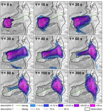
The model was first run at a cell size of 20 m (the same as the DEM resolution) withφ=35◦andδ=22◦, assuming tal-weg 1 (Simulation 1; see Table 3 and Fig. 4). This simulation can be considered as a validation with the parameters used by Crosta et al. (2004). Figure 6 illustrates the distribution of flow depth at selected time intervals from the onset (t=0) tot=300 s, when the flow is assumed having stopped. 86 % of the modelled deposit coincide with the observed area of deposition, and 79 % of the observed deposition area are oc-cupied by the modelled deposit (considering only those areas with depth of deposition>1 m; Table 4). The travel distance modelled for the central part of the deposit corresponds very well to the observation.
However, some issues become obvious from Fig. 6: 1. some portions of the lateral (northern and southern)
1
φ Fig. 6. Time series of flow depth distribution simulated withφ= 35◦andδ=22◦at a cell size of 20 m. Only flow depths>1 m are shown.
Table 4.Correspondence of observed and modelled rock avalanche deposit and key output parameters for each simulation: c1=per cent of surface of modelled deposit with depth≥1 m located within the observed deposition area;c2=per cent of observed deposition area with modelled deposition of depth≥1 m; dmax=maximum depth of modelled deposit;vmax=maximum modelled flow veloc-ity.
c1 c2 dmax vmax
(per cent) (per cent) (m) (m s−1) Simulation 01 86 79 75 94 Simulation 02 73 91 39 86 Simulation 03 93 73 85 96 Simulation 04 87 75 72 88 Simulation 05 85 78 67 107 Simulation 06 74 79 69 80 Simulation 07 84 82 67 97 Simulation 08 82 85 60 99
2. the depth of the deposit is underestimated: whilst the measured maximum depth is approx. 90 m (Govi et al., 2002), the model yields a maximum depth of 75 m only; 3. already shortly after the onset of the flow (t=10 s), the simulation predicts a degree of lateral spreading of the flow beyond the observed extent. As a conse-quence, part of the material crosses the delineation of the catchment and follows gullies north and south of the
1
φ Fig. 7.Time series of flow velocity distribution simulated withφ= 35◦andδ=22◦at a cell size of 20 m.
main flow path, a behaviour not at all observed in real-ity.
The lake dammed by the rock avalanche deposit was mod-elled by filling the sink behind the simulated deposit (see
t=300 in Fig. 6). The extent of the modelled lake corre-sponds well to the observation on 20 September 1987 (see Fig. 3b), which represents the lake close to its maximum ex-tent.
and related processes move at much higher velocities (e.g. Evans et al., 2009a).
The values used forφ andδ – and their spatial distribu-tion in particular – are uncertain. Therefore, the sensitivity of the model to variations of these governing parameters has to be evaluated. r.avalancheis supposed to be sensitive also to changes of the assumed talweg and to the cell size used for the simulation. Table 4 summarizes the key output parame-ters for each simulation and the correspondence of modelled and observed deposit.
4.2.2 Sensitivity to cell size
The simulation was repeated with 40 m (Simulation 2) and 12 m cell size (Simulation 3), leaving the remaining parame-ters unchanged (see Table 3). Longitudinal profiles compar-ing the results to those yielded with 20 m cell size as well as the maps of the simulated deposits are shown in Fig. 8. It was observed that the variations of the cell size do not lead to a substantial change in the behaviour of the simulated rock avalanche. However, with coarser resolution, the spreading of the flow is more pronounced and the simulated flow mass is smoothed, leading to a larger impact area but smaller depth of flow and deposit (see Table 4). With 12 m resolution, the predicted maximum depth of the final deposit (85 m) comes close to the observation (approx. 90 m), whilst with 40 m res-olution, it is clearly underestimated (39 m).
This effect is particularly visible when comparing the re-sults for 40 m and 20 m and much less pronounced between 20 m and 12 m. A maximum flow velocity of 86 m s−1was predicted with 40 m cell size, 96 m s−1with 12 m cell size.
These findings are not surprising as the cell size governs the distance of spreading during each time step of the simu-lation. Tests with channelized debris flows have shown that r.avalancheonly works well if the cell size is much smaller than the width of the flow, otherwise lateral spreading is over-estimated. A cell size of 40 m is definitely too coarse for the simulation of the Val Pola Rock Avalanche. The less pro-nounced difference between the results yielded with 20 m and 12 m suggests that these values are close to the cell size ideal for the simulation of this specific event (choosing a too fine resolution would unnecessarily increase computing time).
4.2.3 Sensitivity to assumption of talweg
Whilst the talweg is clearly defined in the idealized topogra-phy suggested by Gray et al. (1999) and Wang et al. (2004), the identification of the talweg is non-trivial for the real ter-rain. A talweg for the simulation has to be defined manu-ally, based on the geometry and the mechanics of the flow. Assumption 1, used for most of the simulations presented here (see Table 3), builds on the fact that the detached mass first moved towards north before rushing down as a rock avalanche: therefore, the starting point of the talweg
1
φ
Fig. 8. (a)Longitudinal profiles of the flow along the talweg at different time steps withφ=35◦andδ=22◦: comparison of the results for 12 m, 20 m and 40 m cell size – the result for 20 m is also shown proportionally to the terrain;(b)flow depth distribution after t=300 s, computed at three different cell sizes.
is shifted north from the centre line of the affected area (see Fig. 4). Assumption 2 works with a talweg following the cen-tre line of the affected area and was tested against assump-tion 1 (Simulaassump-tion 4). The result (comparison of time series of flow depths) is shown in Fig. 9.
1
φ Fig. 9. Time series of flow depth distribution simulated withφ= 35◦ andδ=22◦ at a cell size of 20 m, assuming talweg 2. The computed flow depth assuming talweg 1 is shown as reference (see Fig. 6).
effects should have been included (Pudasaini et al., 2005a, b, 2008). However, only the curvature in the downslope direc-tion is considered here.
4.2.4 Sensitivity to friction parameters
The simulation was repeated withδ=18◦(Simulation 5) and 26◦(Simulation 6; Fig. 10; see Table 4). The expected effects of reduced flow velocity and resulting delayed motion with increasing values of δ were observed (Fig. 11). With δ=
18◦, the predicted flow velocity peaks at 107 m s−1, withδ
=
26◦it reaches 80 m s−1only. Whilst the simulated maximum travel distance is longer when assuming a lower bed friction (t=40 s andt=60 s in Fig. 10a), the final travel distance at
t=300 s is almost the same withδ=18◦and withδ=22◦ (see Fig. 10b). This phenomenon is explained by the higher tendency of the material to flow back into the main valley with lower bed friction. Also withδ=26◦, the modelled final deposit reaches approx. as far east as in the other simulations. An overall look at the deposits shown in Fig. 10b shows that varying the bed friction angle may result in a highly nonlinear response governed by several factors (see Fig. 10): with δ=18◦, the maximum thickness of the deposit de-creases to 67 m (see Table 4), compared toδ=22◦(75 m), an effect to be attributed primarily to increased lateral spread-ing (north–south direction). Withδ=26◦, part of the flow
1
φ Fig. 10. (a)Longitudinal profiles of the flow at different time steps withφ=35◦: comparison of the results withδ=18, 22 and 26◦ with a cell size of 20 m – the flow depth forδ=22◦is also shown proportionally to the terrain;(b)flow depth distribution att=300 s, computed with three different assumptions ofδ.
material would remain in the transit and even onset area. The deposit in general would therefore assume a much more stretched shape in east–west direction, with a maximum depth of 69 m. However, withδ=26◦, the modelled deposit extends farther south than even withδ=18◦. This counter-intuitive effect illustrates that the numerical model is not de-signed to appropriately describe flows on curved flow paths. In this specific case, this affects only the lateral parts of the flow (flow height≤5 m) in the downstream direction, larger flow heights are modelled in a plausible way.
1
Fig. 11. Velocity profiles along the assumed talweg with different assumptions ofδfor selected time steps and for the maximum over the entire flow. The values are positive in downslope direction (from left to right).
a consequence of the stronger tendency of material with re-duced internal friction to level out and therefore fill up the valley bottom. When assuming higher values ofφ, there is less tendency of the modelled rock avalanche to level out the valley bottom, and the deposit is spread over a larger area, but with a lower maximum depth (67 m forφ=40◦and 60 m for
φ=45◦). For laboratory-scale flows, the effects of the basal and internal friction angles are analyzed in detail in Pudasaini and Kroener (2008).
5 Conclusions
r.avalanche represents a first attempt to implement a physically-based, distributed granular flow model with Open Source GIS. With respect to travel distance and impact ar-eas, the physical model considered and computational tool developed are potentially suitable for real avalanche flows. With its current layout, the model is applicable to large-scale mass movements rather than to channelized debris flows. If the width of the flow would be much smaller than its length, a very small cell size (much smaller than the flow width) would be required in order to avoid an unrealistically high degree of lateral spreading. Such a small cell size, however, would lead to unacceptably long computing times.
1
φ φ
φ
Fig. 12. (a)Longitudinal profiles of the flow at different time steps withδ=22◦: comparison of the results withφ=35, 40 and 45◦ with a cell size of 20 m – the flow depth forφ=35◦is also shown proportionally to the terrain;(b)flow depth distribution after t=300 s for three different assumptions ofφ.
The travel distance and partly also the impact area of the Val Pola Rock Avalanche were well reconstructed without re-calibration of the input parameters. In contrast, the max-imum depth of the deposit was rather underestimated. The friction parameters used by Crosta et al. (2004) in combina-tion with the talweg assumpcombina-tion 1 lead to the most realistic model results regarding travel distance along the talweg and maximum depth of the deposit. However, also the other sim-ulations yield parameters of comparable or, for specific pa-rameters, even better quality (see Table 4). The impact area is best predicted when assumingφ=45◦(Simulation 8). Most simulations failed to reconstruct the northern distal part of the impact area but the travel distance in the central part was predicted very well. The same phenomenon is visible in the simulation results of Crosta et al. (2004), where the under-estimation of the northern portion of the impact area is even more pronounced than in the present work.
12 m and 20 m, so that 20 m cell size is considered accept-able. The modelled flow velocities of all simulations are in the range of published estimates (Crosta et al., 2004) which, however, appear high when compared to those specified for other large and rapid mass movements (see Scheidegger, 1973, for examples).
The quality of the results may be limited by uncertainties in the governing parameters and their spatial patterns. How-ever, as it stands now, there are some limitations of the phys-ical model and the numerphys-ical model used:
– r.avalanche is primarily applicable to granular flows with approximately horizontally projected straight flow lines, as this was a basic assumption in the derivation of the model equations for flows over super-imposed com-plex terrain by Gray et al. (1999). However, this concept can further be extended to more general topographies. Whilst the requirement of a straight flow line is fulfilled by many large mass movements, this assumption fails for most channelized debris or mud flows where the travel distance is much larger than the flow width. For such processes, the Pudasaini and Hutter (2003) model, developed for curved and twisted channels, could be considered (Pudasaini et al., 2005a, b, 2008). An alter-native model for arbitrary topography can also be con-sidered. However, it still needs considerable efforts to develop such a model and to apply it to raster-based GIS;
– entrainment of regolith during the flow is disregarded – in the case of the Val Pola Rock Avalanche, entrainment was not extremely significant. However, in general, en-trainment plays a major role for the travel distance of granular flows (e.g. McDougall and Hungr, 2005; So-villa et al., 2006, 2007; Quan Luna et al., 2012). There-fore, high priority should be given to this aspect when pushing the model development further;
– the role of pore water for the motion of the flow is ne-glected, but many geophysical mass flows in nature are a mixture of solid and fluid components and should be considered as such (Iverson and Denlinger, 2001; Puda-saini et al., 2005a).
Attacking the limitations in a comprehensive way will re-quire at least the following steps:
1. selecting and adapting a sound method for modelling rapid granular flows over arbitrary topography, using and extending the existing theories. Such an approach would have to build on the latest extensions of the Savage-Hutter model (Luca et al., 2009a, b, c, d), incor-porating particle entrainment and the role of pore fluid (besides water, also air may play an important role). As explained in Pudasaini (2011a), the rheological model should take into account different dominant physical as-pects as observed in two-phase geophysical mass flows.
Such aspects include the solid volume fraction gradient enhanced non-Newtonian fluid extra stress; the gener-alized interfacial momentum transfer that takes into ac-count the viscous drag, buoyancy, and the virtual mass; and also the generalized drag which covers both the solid-like and fluid-like contributions. Such a general model is essential to describe e.g. complex landslide-river/lake interactions.
2. devising an appropriate high resolution shock capturing numerical scheme for solving the differential equations derived in (1)–(3). Numerical solutions of the avalanche model equations for arbitrary topography would have to be elaborated (e.g. Bouchut and Westdickenberg, 2004; Pudasaini et al., 2005a, b, 2008);
3. performing more simulation tests and calibrating the model with well-studied granular flow events.
Since no user-friendly Open Source software for the motion of granular flows (fully incorporating the relevant physical and geometrical processes) is available at present, the fur-ther development ofr.avalanchein terms of the above points would be highly relevant for reliable process modelling and the delineation of hazard zones.
Acknowledgements. This work was supported by the Tyrolean Science Funds. Special thanks for fruitful discussions go to Kolumban Hutter, Jean F. Schneider, and Mechthild Thalhammer.
Edited by: T. Glade
Reviewed by: J. Blahut and S. P. Pudasaini
References
Blahut, J., Horton, P., Sterlacchini, S., and Jaboyedoff, M.: De-bris flow hazard modelling on medium scale: Valtellina di Tirano, Italy, Nat. Hazards Earth Syst. Sci., 10, 2379–2390, doi:10.5194/nhess-10-2379-2010, 2010.
Bouchut, F. and Westdickenberg, M.: Gravity driven shallow water models for arbitrary topography, Comm. Math. Sci., 2, 359–389, 2004.
Burton, A. and Bathurst, J. C.: Physically based modelling of shallow landslide sediment yield at a catchment scale, Environ. Geol., 35, 89–99, 1998.
Cannata, M. and Molinari, M.: Natural Hazards and Risk Assess-ment: The FOSS4G Capabilities. Academic Proceedings of the 2008 Free and Open Source Software for Geospatial (FOSS4G) Conference, 29 Sept.–3 Oct., Cape Town, South Africa, 172– 181, 2008.
Chau, K. T. and Lo, K. H.: Hazard assessment of debris flows for Leung King Estateof Hong Kong by incorporating GIS with nu-mericalsimulations, Nat. Hazards Earth Syst. Sci., 4, 103–116, doi:10.5194/nhess-4-103-2004, 2004.
Christen, M., Kowalski, J., and Bartelt, B.: RAMMS: Numerical simulation of dense snow avalanches in three-dimensional ter-rain, Cold Reg. Sci. Technol., 63, 1–14, 2010b.
Corominas, J., Copons, R., Vilaplana, J. M., Altamir, J., and Amig´o, J.: Integrated Landslide Susceptibility Analysis and Hazard As-sessment in the Principality of Andorra, Nat. Hazards, 30, 421– 435, 2003.
Crosta, G. B., Imposimato, S., and Roddeman, D. G.: Numerical modelling of large landslides stability and runout, Nat. Hazards Earth Syst. Sci., 3, 523–538, doi:10.5194/nhess-3-523-2003, 2003.
Crosta, G. B., Chen, H., and Lee, C. F.: Replay of the 1987 Val Pola Landslide, Italian Alps, Geomorphology, 60, 127–146, 2004. Dietrich, W. E. and Montgomery, D. R.: SHALSTAB: A Digital
Terrain Model for Mapping Shallow Landslide Potential, Na-tional Council of the Paper Industry for Air and Stream Improve-ment, Technical Report, 1998.
Evans, S. G., Bishop, N. F., Fidel Smoll, L., Valderrama Murillo, P., Delaney, K. P., and Oliver-Smith, A.: A re-examination of the mechanism and human impact of catastrophic mass flows orig-inating on Nevado Huascar´an, Cordillera Blanca, Peru in 1962 and 1970, Eng. Geol., 108, 96–118, 2009a.
Evans, S. G., Roberts, N. J., Ischuk, A., Delaney, K. B., Morozova, G. S., and Tutubalina, O.: Landslides triggered by the 1949 Khait earthquake, Tajikistan, and associated loss of life, Eng. Geol., 109, 195–212, 2009b.
Gamma, P.: Dfwalk – Murgang-Simulationsmodell zur Gefahren-zonierung, Geographica Bernensia, G66, 144 pp., 2000. Godt, J. W., Baum, R. L., Savage, W. Z., Salciarini, D., Schulz,
W. H., and Harp, E. L.: Transient deterministic shallow land-slide modeling: Requirements for susceptibility and hazard as-sessments in a GIS framework, Eng. Geol., 102, 214–226, 2008. Govi, M., Gull`a, G., and Nicoletti, P. G.: Val Pola rock avalanche of July 28, 1987, in Valtellina (Central Italian Alps), in: Catas-trophic landslides: Effects, occurrence, and mechanism, edited by: Evans, S. G. and Degraff, J. V., Geol. Soc. Am. Rev. Eng. Geol., 15, 71–89, 2002.
GRASS Development Team: Geographic Resources Analysis Sup-port System (GRASS) Software, Open Source Geospatial Foun-dation Project, available at: http://grass.osgeo.org, last access: 27 December 2011, 2011.
Gray, J. M. N. T., Wieland, M., and Hutter, K.: Gravity-driven free surface flow of granular avalanches over complex basal topogra-phy, Proc. R. Soc. Lond. A, 455, 1841–1874, 1999.
Guzzetti, F., Galli, M., Reichenbach, P., Ardizzone, F., and Cardi-nali, M.: Landslide hazard assessment in the Collazzone area, Umbria, Central Italy, Nat. Hazards Earth Syst. Sci., 6, 115–131, doi:10.5194/nhess-6-115-2006, 2006.
Highland, L. M. and Bobrowsky, P.: The landslide handbook. A guide to understanding landslides, US Geological Survey Circu-lar, 1325, 129 pp., 2008.
Hungr, O.: A model for the runout analysis of rapid flow slides, de-bris flows, and avalanches, Can. Geotech. J., 32, 610–623, 2005. Hungr, O., Corominas, J., and Eberhardt, E.: State of the Art pa-per: Estimating landslide motion mechanism, travel distance and velocity, in: Landslide Risk Management, edited by: Hungr, O., Fell, R., Couture, R., and Eberhardt, E., Proceedings of the Inter-national Conference on Landslide Risk Management, Vancouver, Canada, 31 May–3 June 2005, 129–158, 2005.
Iverson, R. M.: The physics of debris flows, Rev. Geophys., 35, 245–296, 1997.
Iverson, R. M. and Denlinger, R. P.: Flow of variably fluidised gran-ular masses across three-dimensional terrain, I: Coulomb mixture theory, J. Geophys. Res., 106, 537–552, 2001.
Jarvis, A., Reuter, H. I., Nelson, A., and Guevara, E.: Hole-filled seamless SRTM data V4, International Centre for Tropical Agri-culture (CIAT), available at: http://srtm.csi.cgiar.org, last access: 9 January 2012, 2008.
Kappes, M. S., Malet, J.-P., Remaˆıtre, A., Horton, P., Jaboyedoff, M., and Bell, R.: Assessment of debris-flow susceptibility at medium-scale in the Barcelonnette Basin, France, Nat. Hazards Earth Syst. Sci., 11, 627–641, doi:10.5194/nhess-11-627-2011, 2011.
Lee, S.: Application of Likelihood Ratio and Logistic Regression Models to Landslide Susceptibility Mapping Using GIS, Envi-ron. Manage., 34, 223–232, 2004.
Lied, K. and Bakkehøi, S.: Empirical calculations of snow-avalanche run-out distance based on topographic parameters, J. Glaciol., 26, 165–177, 1980.
Luca, I., Hutter, K., Tai, Y. C., and Kuo, C. Y.: A hierarchy of avalanche models on arbitrary topography, Acta Mech., 205, 121–149, 2009a.
Luca, I., Hutter, K., Tai, Y. C., and Kuo, C. Y.: Two-layer models for shallow avalanche flows over arbitrary variable topography, Int. J. Adv. Engin. Sci. Appl. Math., 1, 99–121, 2009b.
Luca, I., Tai, Y. C., and Kuo, C. Y.: Modelling shallow-gravity driven solid-fluid mixtures over arbitrary topography, Comm. Math. Sci., 7, 1–36, 2009c.
Luca, I., Tai, Y. C., and Kuo, C. Y.: Non-Cartesian topogra-phy based avalanche equations and approximations of gravity driven flows of ideal and viscous fluids, Math. Mod. Meth. Appl. Sci., 19, 127–171, 2009d.
McClung, D. M. and Lied, K.: Statistical and geometrical definition of snow avalanche runout, Cold Regions Sci. Technol., 13, 107– 119, 1987.
McDougall, S. and Hungr, O.: A Model for the Analysis of Rapid Landslide Motion across Three-Dimensional Terrain, Can. Geotech. J., 41, 1084–1097, 2004.
McDougall, S. and Hungr, O.: Dynamic modeling of entrainment in rapid landslides, Can. Geotech. J., 42, 1437–1448, 2005. Mergili, M. and Fellin, W.: Three-dimensional modelling of
rota-tional slope failures with GRASS GIS, Proceedings of the 2nd World Landslide Forum, Rome, October 3–9, 2011.
Mergili, M. and Schneider, J. F.: Regional-scale analysis of lake outburst hazards in the southwestern Pamir, Tajikistan, based on remote sensing and GIS, Nat. Hazards Earth Syst. Sci., 11, 1447– 1462, doi:10.5194/nhess-11-1447-2011, 2011.
Mergili, M., Fellin, W., Moreiras, S. M., and St¨otter, J.: Simulation of debris flows in the Central Andes based on Open Source GIS: Possibilities, limitations, and parameter sensitivity. Nat. Hazards, in press, doi:10.1007/s11069-011-9965-7, 2011.
Nessyahu, H. and Tadmor, E.: Non-oscillatory central differencing for hyperbolic conservation laws, J. Comput. Phys., 87, 408–463, 1990.
Congress of the International Association of Engineering Geol-ogy, Vancouver, British Columbia, Canada, 21–25 Sept. 1998, 8 pp., 1998.
Perla, R., Cheng, T. T., and McClung, D. M.: A Two-Parameter Model of Snow Avalanche Motion, J. Glaciol., 26, 197–207, 1980.
Pitman, E. B., Nichita, C. C, Patra, A. K, Bauer, A. C., Bursik, M., and Weber, A.: A model of granular flows over an erodible sur-face, Discrete Contin. Dynam. Syst. B., 3, 589–599, 2003. Pudasaini, S. P.: Dynamics of Flow Avalanches Over Curved and
Twisted Channels. Theory, Numerics and Experimental Valida-tion, Dissertation at the Technical University of Darmstadt, Ger-many, 2003.
Pudasaini, S. P.: A General Two-Fluid Debris Flow Model, Geo-phys. Res. Abstr. 13, EGU2011-4205-1, 2011a.
Pudasaini, S. P.: Some exact solutions for debris and avalanche flows, Phys. Fluids, 23, 043301, doi:10.1063/1.3570532, 2011b. Pudasaini, S. P. and Hutter, K.: Rapid shear flows of dry granular masses down curved and twisted channels, J. Fluid Mech., 495, 193–208, 2003.
Pudasaini, S. P. and Hutter, K.: Avalanche Dynamics: Dynamics of rapid flows of dense granular avalanches, Springer, Berlin Hei-delberg New York, 2007.
Pudasaini, S. P. and Kroener, C.: Shock waves in rapid flows of dense granular materials: theoretical predictions and experimental results, Phys. Rev. E, 78, 041308, doi:10.1103/PhysRevE.78.041308, 2008.
Pudasaini, S. P., Wang, Y., and Hutter, K.: Modelling debris flows down general channels, Nat. Hazards Earth Syst. Sci., 5, 799– 819, doi:10.5194/nhess-5-799-2005, 2005a.
Pudasaini, S. P., Wang, Y., and Hutter, K.: Rapid motions of free-surface avalanches down curved and twisted channels and their numerical simulation, Phil. Trans. R. Soc. A, 363, 1551–1571, 2005b.
Pudasaini, S. P., Hutter, K., Hsiau, S.-S., Tai, S.-C., Wang, Y., and Katzenbach, R.: Rapid flow of dry granular materials down in-clined chutes impinging on rigid walls, Phys. Fluids, 19, 053302, doi:10.1063/1.2726885, 2007.
Pudasaini, S. P., Wang, Y., Sheng, L.-T., Hsiau, S.-S., Hutter, K., and Katzenbach, R.: Avalanching granular flows down curved and twisted channels: Theoretical and experimental results, Phys. Fluids, 20, 073302, doi:10.1063/1.2945304, 2008. Quan Luna, B., Remaˆıtre, A., van Asch, Th. W. J., Malet, J.-P., and
Van Westen, C. J.: Analysis of debris flow behavior with a one di-mensional run-out model incorporating entrainment, Eng. Geol., in press, doi:10.1016/j.enggeo.2011.04.007, 2012.
Revellino, P., Guadagno, F. M., and Hungr, O.: Morphological methods and dynamic modelling in landslide hazard assessment of the Campania Apennine carbonate slope, Landslides, 5, 59– 70, 2008.
Rickenmann, D.: Empirical Relationships for Debris Flows, Nat. Hazards, 19, 47–77, 1999.
Sampl, P. and Zwinger, T.: Avalanche Simulation with SAMOS, Ann. Glaciol., 38, 393–398, 2004.
Savage, S. B. and Hutter, K.: The motion of a finite mass of granu-lar material down a rough incline, J. Fluid Mech., 199, 177–215, 1989.
Scheidegger, A. E.: On the Prediction of the Reach and Velocity of Catastrophic Landslides, Rock Mech., 5, 231–236, 1973. Scheidl, C. and Rickenmann, D.: Empirical prediction of
debris-flow mobility and deposition on fans, Earth Surf. Proc. Land-forms, 35, 157–173, 2010.
Sovilla, B., Burlando, P., and Bartelt, P.: Field experiments and numerical modeling of mass entrainment in snow avalanches, J. Geophys. Res., 111, F03007, doi:10.1029/2005JF000391, 2006. Sovilla, B., Margreth, S., and Bartelt, P.: On snow entrainment in avalanche dynamics calculations, Cold Reg. Sci. Technol., 47, 69–79, 2007.
Tai, Y. C., Noelle, S., Gray, J. M. N. T., and Hutter, K.: Shock-capturing and front-tracking methods for granular avalanches, J. Comput. Phys., 175, 269–301, 2002.
Takahashi, T., Nakagawa, H., Harada, T., and Yamashiki, Y.: Rout-ing debris flows with particle segregation, J. Hydrol. Res., 118, 1490–1507, 1992.
Van Westen, C. J., van Asch, T. W. J., and Soeters, R.: Landslide hazard and risk zonation : why is it still so difficult?, Bull. Eng. Geol. Environ, 65, 176–184, 2005.
Vandre, B. C.: Rudd Creek debris flow, in: Delineation of landslide, flash flood and debris flow hazards in Utah, edited by: Bowles, D. S., 117–131, Utah Water Research Laboratory, 1985.
Voellmy, A.: ¨Uber die Zerst¨orungskraft von Lawinen, Schweiz-erische Bauzeitung, 73, 159–162, 212–217, 246–249, 280–285, 1955.
Wang, Y., Hutter, K., and Pudasaini, S. P.: The Savage-Hutter the-ory: A system of partial differential equations for avalanche flows of snow, debris, and mud, J. Appl. Math. Mech., 84, 507– 527, 2004.
Wichmann, V. and Becht, M.: Modelling of Geomorphic Processes in an Alpine Catchment, in: Proceedings of the 7th International Conference on GeoComputation, Southampton, 14 pp., 2003. Zwinger, T., Kluwick, A., and Sampl, P.: Numerical simulation of