204 Hygor Amaral Santana et al.
Modelos para predição da área foliar individual de leguminosas forrageiras
A área foliar é uma variável essencial para a quantificação de outras importantes características foliares em estudos fisiológicos de plantas, como taxa fotossintética e teor de fósforo, normalizados por área. Essa é uma das razões para a necessidade de métodos rápidos e precisos para estimar a área foliar. O objetivo deste trabalho foi ajustar modelos de regressão linear ou não linear para predizer a área foliar de seis espécies de leguminosas forrageiras, a partir de imagens digitais analisadas com o pacote LeafArea, software R. Em um experimento de campo, foram coletadas aleatoriamente 100 folhas das seguintes espécies: Crotalaria juncea (L.), Canavalia ensiformis (L.), Cajanus cajan (L.), Dolichos lablab (L.), Mucuna cinereum (L.), e Mucuna aterrima (Piper & Tracy) Merr., nas quais foram medidos o comprimento e a largura do folíolo central. Posteriormente, imagens digitais de cada folha foram processadas no software R para estimativa da área foliar. Essas estimativas foram usadas para ajustar modelos de predição de área foliar; de fato, setenta folhas foram usadas para ajustar os modelos; o restante delas foi usado para validação do modelo. Para as seis espécies, o modelo polinomial completo de segundo grau, ou submodelos derivados, pode ser usado para predizer a área foliar em função do comprimento e largura do folíolo central, apresentando R² acima de 0,98 e porcentagem de erro médio absoluto abaixo de 9%. Nestes modelos, o efeito da largura da folha é geralmente maior que o comprimento da folha. O pacote R LeafArea mostrou-se uma ferramenta muito eficiente para a estimativa da área foliar através da execução do software ImageJ, com alta precisão e fácil calibração.
Palavras-chave: Fabaceae; comprimento da folha; largura da folha; pacote LeafArea, imagens digitais.
ABSTRACT
RESUMO
Short communication
Models for prediction of individual leaf area of forage legumes
Leaf area is an essential variable for the quantification of other important leaf characteristics in physiological studies of plants, such as normalized photosynthetic rate and normalized phosphorus content. That is one of the reasons for the need of fast and accurate methods to estimate leaf area. The objective of this work was to fit linear or non-linear regression models to predict the individual leaf area of six species of forage legumes, based on digital images analyzed with the package LeafArea, R software. In a field experiment, 100 leaves were randomly collected from the following species: Crotalaria juncea (L.), Canavalia ensiformis (L.), Cajanus cajan (L.), Dolichos lablab (L.), Mucuna cinereum (L.), and Mucuna aterrima (Piper & Tracy) Merr., in which the central leaflet length and width were measured. Afterwards, digital images of each leaf were processed in R software for leaf area estimation. These estimates were used to fit leaf area prediction models; in fact, seventy leaves were used to fit the models; the rest of them were used for model validation. For the six species, the complete second-degree polynomial model, or derivative submodels, can be used to predict leaf area as a function of length and width of the central leaflet, presenting R² above 0.98 and percentage absolute mean error below 9%. In these models, the effect of leaf width is generally greater than the leaf length. The R package LeafArea showed to be a very efficient tool for the estimation of leaf area through the execution of the software ImageJ, with high precision and easy calibration.
Keywords: Fabaceae; leaf length; leaf width; package LeafArea; digital images.
Hygor Amaral Santana1, Brunna Rithielly Rezende1, Wilhan Valasco dos Santos1, Anderson Rodrigo da Silva1* 10.1590/0034-737X201865020013
licence Creative Commons
Submitted on August 02nd, 2017 and accepted on March 22nd, 2018.
INTRODUCTION
Forage legumes (Fabaceae family), such as lablab (Dolichos lablab L.) and crotalaria (Crotalaria juncea L.), are widely cultivated as green fertilizers because of their biological and nitrogen-fixation capacity in the soil (Philippot et al., 2013), which increases the availability of this nutrient for conventional crops (e.g. maize). These plants provide a very efficient plant cover (Perin et al., 2004), help to control weeds (Monquero et al., 2009), provide animal feed (Fiallos et al., 2012) and soil protection against mechanical damage, and avoid losses of nutrients by leaching and/or percolation (Souza et al., 2012). Nevertheless, the production of biomass and the efficient use of these species are directly related to the foliage production.
Leaf area is a commonly analyzed variable in field studies (Wang & Zhang, 2012) with woody species, agricultural crops, and weeds. This is because several leaf characteristics are typically normalized by leaf area, such as maximum rate of net photosynthesis, dark respiration rate, nitrogen content, and phosphorus content (Osnas et al., 2013). In phytopatometry, the calculation of leaf area through image analysis is essential to evaluate the severity of diseases, substituting disease diagrammatic scales, and pest damage degree. However, accurate measurements of leaf area usually require the use of expensive equipment, making this type of procedure unviable, especially in large scale.
There are also indirect, non-destructive, methods of foliar area measurement, thus circumventing logistical difficulties in obtaining data. These methods consist in the application of dimensional or allometric analysis from mathematical equations that relate linear measures of the leaf limb to its area (Marchi et al., 2011). In general, these methods are simple, efficient, and inexpensive, based on linear models (Souza & Amaral, 2015), avoiding leaf exception, thus eliminating the need for foliar area meters or geometric reconstructions.
Nowadays, digital cameras are promising devices for the measurement of leaf area in field because they are easy to handle, cheaper than leaf measuring devices, and perhaps more accurate than methods based on leaf dimensions, especially when leaves present damage (Godoy et al., 2007). The estimation of leaf area through digital images has already been performed with several species, such as legumes (Cargnelutti Filho et al., 2015; Cargnelutti Filho et al., 2012; Toebe et al., 2012), soybean
(Richter et al., 2014), common bean (Martin et al., 2013), grasses (Zanchi et al., 2009), and perennial crops (Godoy et al., 2007).
The package LeafArea (Katabuchi, 2015) of the R software (R Core Team, 2016) allows to conveniently exe-cute the software ImageJ (Rasband, 2016; Schneider et al., 2012) for the analysis of digital images. The package provides an easy-to-use automated tool to measure the leaf area of several images simultaneously, but requires the excision of leaves, not allowing the same leaves to be measured later (Rouphael et al., 2010).
The objective of this work was to fit regression models, linear or non-linear, to predict the individual leaf area of six cultivated species of forage legumes, based on digital images analyzed with the R package LeafArea.
MATERIAL AND METHODS
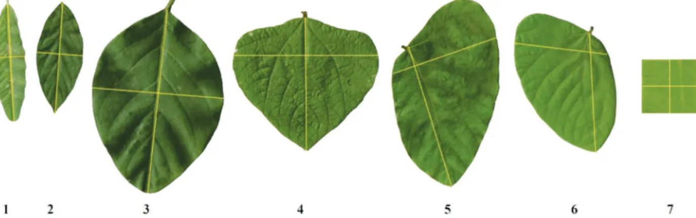
The experiment was carried out in an experimental area in Urutaí, GO, Brazil (latitute: 17°29’24.4" S, longitude: 48°13’3.2" W), where the following crops were grown: Crotalaria juncea (L.) cv. IAC-KR1, Canavalia ensiformis (L.), Cajanus cajan (L.) cv. IAPAR 43 - Aratã, Dolichos lablab (L.) cv. Rongai, Mucuna cinereum (L.), and Mucuna aterrima (Piper & Tracy) Merr., all spaced 0.5 m between rows. When the plants were in full bloom, 100 leaves of the middle third of each cultivar were randomly collected. Each leaf was composed of three leaflets.
In these 100 leaves, we measured, with a millimeter ruler, the length and the width of the central leaflet, as illustrated in Figure 1. The central leaflets were scanned using an HP Ink Advantage 1516® multifunctional digital printer, generating A4 size images (210 × 297 mm). Then, the images were processed and analyzed with the package LeafArea version 0.1.1 for leaf area estimation through the function run.ij() that automatically runs ImageJ. Images are initially segmented to separate background from leaf blade. The proportion of pixels in each part of the segmented image is computed and used to calculate leaf area. To calibrate the function, a leaf cut of 5 × 5 cm size was scanned and processed, setting the arguments “distance.pixel = 395.02” and “known.distance = 5.0”. To prevent dust from affecting the image analysis, the size lower limit for leaf area to be considered on calculations was set to 4.5 (cm², in this case), through the argument “low.size”.
An exploratory analysis of the length, width, and leaf area data from the 100 leaflets of each species was
Table 1: Models to predict leaf area (LA) as a function of the length (L) and width (W) of the central leaflet
Model Function
Power LA = L Wβ1 β2 + ε
2
performed, calculating minimum, mean, and maximum values. Then, 70 leaves of each species were used to fit the regression models described in Table 1, to predict the leaf area as a function of leaflet length and width.
The complete second-degree polynomial model was also subjected to the stepwise selection of regressors, aiming to obtain more parsimonious submodels.
We highlight that all models were fitted without the intercept, so that for null values of length and width, the leaf area would also be zero. The choice of model for each species was based on the goodness-of-fit criteria presented
in Table 2. After choosing the model, 30% of the data (30 leaves of each species) were used for the validation of the model, computing Pearson’s correlation coefficient between observed and predicted values. Shepard diagrams were built to visualize this relationship.
All statistical analyzes were performed with the software R (R Core Team, 2016).
RESULTS AND DISCUSSION
The crops have a great diversity of leaf formats and dimensions. C. ensiformis showed the highest leaf area, followed by M. cinereum, M. aterrima, D. lablab, C. juncea, and C. cajan (Table 3). In each of the six species, the variability in terms of leaf area varied from 20 to 35%. The fitted equations that relate the leaf area with length and width, as well as the goodness-of-fit criteria, are presented in Table 4. In bold, we highlighted the chosen model, also considering the complexity of the model. It was observed, for example, that for C. juncea, the reduced linear model practically did not present reduction in R² and adjusted coefficient of determination (R²aj). or increase in mean absolute percentage error (MAPE) and AIC.
Different models were required for the leaf area according to the species. However, it is known (Maldaner et al., 2009; Monteiro et al., 2005; Queiroga et al., 2003) that the format, age, and size of the leaves determine the type of model used for leaf area prediction.
Figure 1: Scanned images of central leaflet of 1) C. juncea, 2) C. ensiformis, 3) C. cajan, 4) D. lablab, 5) M. cinereum, 6) M. aterrima, and 7) foliar cut 5 × 5 cm.
Table 3: Minimum, maximum, and mean (n = 100) values of leaflet length, width, and area
Length (cm) Width (cm) Leaf area (cm²)
Min. Max. Mean Min. Max. Mean Min. Max. Mean
C. juncea 9.31 19.15 12.42 2.02 5.12 3.13 16.07 73.89 31.37 C. ensiformis 11.85 21.37 16.74 8.76 17.72 12.30 78.42 275.86 160.13 C. cajan 6.71 12.46 9.39 2.48 6.08 4.12 12.71 51.79 29.21
D. Lablab 7.62 14.09 11.05 7.85 15.20 12.12 46.18 151.32 98.26
M. cinereum 10.09 17.72 14.59 8.97 15.91 12.07 86.94 238.22 144.64
M. aterrima 9.31 18.36 13.41 7.77 14.55 10.56 46.92 210.14 114.53 Species
Table 2: Goodness-of-fit criteria
Criterion Equation
Coefficient of determination
Adjusted coefficient of determination ( - 1) - R n p
2
n - p - 1
R2aj =
Mean absolute percentage error MAPE = 100n
n
i = 1
|^ |εi
LAi
Akaike’s information criterion AIC = p - logL2 ( ( ))
SSR - residual sum of squares; SST - total sum of squares; p - number of model parameters; n - number of observations (70, in this case);
LAi - i-th value of leaf area; ogL( )) - maximum value of the likelihood
Table 4: Fitted models to predict leaf area (LA) as a function of leaflet length (L) and width (W)
Species Fitted model R² R²aj. MAPE AIC
LA = 1.37763L - 4.83394W - 0.10460L² - 0.46837W² + 1.26844(L×W) 0.9989 0.9988 2.94 313.71 C. juncea LA = 0.35959L - 0.91680W + 0.74287(L×W) 0.9988 0.9988 2.99 314.05
LA = L0.91256 × W0.98504 0.9877 0.9875 3.32 337.06
LA = -8.268L + 14.141W + 2.351L² + 3.085W² - 4.881(L×W) 0.9907 0.9902 6.13 847.90 C. ensiformis LA = 1.7628L² + 2.8624W² - 3.7505(L × W) 0.9900 0.9897 6.05 850.95
LA = L1.2882 × W0.5714 0.8074 0.8054 5.87 848.29
LA = -0.85546L + 2.81942W + 0.16528L² + 0.39295W² + 0.09497(L×W) 0.9990 0.9989 2.42 285.25
C. cajan — — — — —
LA = L0.85813 × W1.0103 0.9892 0.9891 2.42 280.37
LA = -2.1384L + 2.9399W + 0.9479L² + 0.4828W² - 0.7655(L×W) 0.9983 0.9982 3.49 577.72
D. Lablab LA = 0.780226L² 0.9923 0.9922 7.33 724.05
LA = L1.11188 × W0.76304 0.9695 0.9692 3.56 577.50
LA = 2.4854L - 1.9488W + 0.6807L² + 0.5324W² - 0.5240(L×W) 0.9859 0.9852 9.00 869.27
M. cinereum — — — — —
LA = L1.5531 × W0.3228 0.7236 0.7208 8.94 863.56
LA = 14.7211L - 18.8437W - 0.1182L² + 1.4295W² - 0.1730(L×W) 0.9911 0.9906 8.39 778.71
M. aterrima — — — — —
LA = L0.9104 × W1.0044 0.8697 0.8697 8.67 777.73
MAPE - mean absolute percentage error; AIC - Akaike’s information criterion; R2 - coefficient of determination; R²
aj. - adjusted coefficient
of determination.
It was not possible to obtain a reduced linear model for C. cajan and the two mucunas. A power model was chosen for C. cajan. Due to expressive differences in R² and R²aj, we chose the complete linear model for M. cinereum and M. aterrima.
Except for D. lablab, the product (L × W) was necessary in all prediction equations (Table 4). The fitted model for D. lablab was a reduced polynomial, with only the quadratic effect of leaf length, LA = 0.780226L². And this is perfectly plausible, given the more rounded shape of the leaflet (Figure 1). Note that if we take the simple ratios between the mean length and width of each species found in Table 3, we will see that the one of D. lablab is closest to 1 (11.05/12.12 = 0.91), showing a greater circularity. Thus, it would be unnecessary to have both variables (length and width) in the same model. In addition, based on the area of the circle, we approach the coefficient of the fitted equation, that is,
L
2
2 π
4
Lucena et al. (2011) found that linear models are optimal for estimating leaf area of acerola. Sachet et al. (2015) observed that the best method to estimate leaf area of peach is the linear model, replacing the destructive analysis. For M. cinereum (Cargnelutti Filho et al., 2012) and C. ensiformis (Toebe et al., 2012), linear models using leaf width and length were well fitted, presenting R² of 0.992 and 0.978, respectively, corroborating the results found here.
The linear effect of the width is higher than the leaf length (Table 4). In the case of M. cinereum, the length had a slightly higher effect. Toebe et al. (2012) observed that the width of the central leaflet of C. ensiformis affects leaf area more than the leaf length. Cargnelutti Filho et al. (2012) reported that the leaf area of M. cinereum is more affected by width.
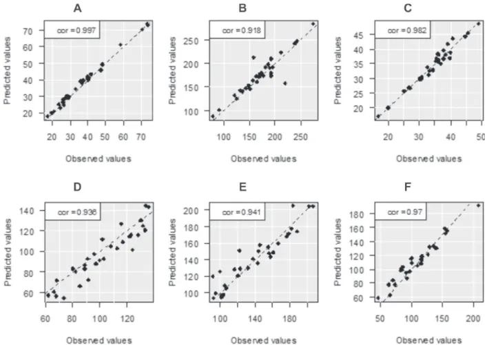
Figure 2 shows Shepard diagrams of the observed values of leaf area and values predicted by the chosen model with the data of 30 leaves, randomly chosen from each species, to validate the fitted model. The correlation coefficients were all higher than 0.93, indicating high reliability of the models.
CONCLUSIONS
For the six species, the complete second-degree polynomial model, or derivative submodels, can be used to predict the leaf area as a function of length and width of the central leaflet, presenting high goodness-of-fit, with R² above 0.98 and mean absolute percentage error below 9%. In these models, the effect of leaf width is generally greater than the leaf length.
The four criteria of goodness-of-fit, coefficient of determination, mean absolute percentage error, and Akaike’s information criterion, were generally concordant with each other. Nevertheless, Akaike’s information criterion was more sensitive to the number of parameters than the adjusted coefficient of determination.
The R package LeafArea showed to be a very efficient application for the estimation of leaf area through the execution of software ImageJ, with high precision and easy calibration.
ACKNOWLEDGEMENTS
We thank the Instituto Federal Goiano (Brazil), for the financial support, and NEPA – Núcleo de Estudos e Pes-quisas em Agroecologia (IF Goiano, Urutaí, GO, Brazil), for supplying the seeds.
REFERENCES
Cargnelutti Filho A, Toebe M, Burin C, Fick AL, Neu IMM & Facco G (2012) Leaf area estimation of velvet bean through non destructive method. Ciência Rural, 42:238-242.
Cargnelutti Filho A, Toebe M, Alves BM & Burin C (2015) Leaf area estimation of pigeonpea by leaf dimensions. Ciência Ru-ral, 45:01-08.
Fiallos FG, Silva WM & Benavides OP (2012) Germination and health quality of mucuna white and black seeds used as a green manure in Quevedo, Ecuador. Scientia Agropecuaria, 3:15-21.
Godoy LJG, Yanagiwara RS, Bôas RLV, Backes C & Lima CP (2007) Digital image analysis for estimatives of leaf area in “Pêra” orange plants. Revista Brasileira de Fruticultura, 29:420-424.
Katabuchi M (2015) LeafArea: an R package for rapid digital image analysis of leaf area. Ecological Research., 30:1073-1077.
Lucena RRM, Batista TMV, Dombroski JLD, Lopes WAR & Rodrigues GSO (2011) Measurement of acerola leaf area. Re-vista Caatinga, 24:40-45.
Maldaner IC, Heldwein AB, Loose LH, Lucas DDP, Guse FI & Bortoluzzi MP (2009) Models for estimating leaf area in sunflower. Ciência Rural, 39:1356- 1361.
Marchi SR, Martins D & Costa NV (2011) Non-destructive method for surface leaf area estimate of weeds from aquatic environments: african tanner-grass and capim-fino. Semina: Ciências Agrárias, 32:1717-1724.
Martin TN, Marchese JA, Sousa AKF, Curti GL, Fogolar IH & Cunha VS (2013) Using the ImageJ software to estimate leaf area in bean crop. Interciencia, 38:843-848.
Monquero PA, Amaral LR, Inácio EM, Brunhara JP, Binha DP, Silva PV & Silva AC (2009) Effect of green fertilizers on the suppression of different species of weeds. Planta Daninha, 27:85 95.
Monteiro JEBA, Sentelhas PC, Chiavegato EJ, Guiselini C, Santi-ago AV & Prela A (2005) Cotton leaf area estimates based on leaf dimensions and dry mass methods. Bragantia, 64:15-24.
Perin A, Santos RHS, Urquiaga S, Guerra JGM & Cecon PR (2004) Phytomass yield, nutrients accumulation and biological nitrogen fixation by single and associated green manures. Pesquisa Agropecuária Brasileira, 39:35-40.
Philippot L, Raaijmakers JM, Lemanceau P & Vanderputten WH (2013) Going back to the roots: the microbial ecology of the rhizosphere. Nature Reviews Microbiology, 11:789-799.
Queiroga JL, Romano EDU, Souza JRP & Miglioranza E (2003) Model to estimate the leaf area of snap bean. Horticultura Bra-sileira, 21:64-68.
R Core Team (2016) R: A Language and environment for statistical computing. Disponível em: <www.R-project.org>. Accessed em: 18 de junho de 2016.
Rasband WS (2016) ImageJ. Available at: <http://imagej.nih.gov/ ij/>. Accessed em: 01 de abril de 2017.
Richter GL, Zanon Júnior A, Streck NA, Guedes JVC, Kräulich B, Rocha TSM, Winck JEM & Cera JC (2014) Estimating leaf area of modern soybean cultivars by a non-destructive method. Bragantia, 73:416-425.
Rouphael Y, Mouneimne AH, Ismail A, Gyves EM, Rivera CM & Colla G (2010) Modeling individual leaf area of rose (Rosa hybrida L.) based on leaf length and width measurement. Photosynthetica, 48:09-15.
Sachet MR, Penso GA, Pertille RH, Guerrezi MT & Citadini I (2015) Non-destructive leaf area estimation in peach tree. Ciência Rural, 45:2161-2163.
Schneider CA, Rasband WS & Eliceiri KW (2012) NIH Image to ImageJ: 25 years of image analysis. Nature Methods, 9:671-675.
Souza MC & Amaral CL (2015) Non-destructive linear model for leaf area estimation in Vernonia ferruginea Less. Brazilian Journal of Biology, 75:152-156.
Souza MC, Pires FR, Partelli FL & Assis RL (2012) Adubação verde e rotação de culturas. Viçosa, UFV. 108p.
Toebe M, Cargnelutti Filho A, Burin C, Fick AL, Neu IMM, Casarotto G & Alves BM (2012) Leaf area prediction models for jack bean by leaf dimensions. Bragantia, 71:37-41.
Wang Z & Zhang L (2012) Leaf shape alters the coefficients of leaf area estimation models for Saussurea stoliczkai in central Tibet. Photosynthetica, 50:337-342.