Mathematical modelling of shallow flows: Closure
models drawn from grain-scale mechanics of
sediment transport and flow hydrodynamics
1
Rui M. L. Ferreira, Ma´rio J. Franca, Joa˜o G. A. B. Leal, and Anto´nio H. Cardoso
Abstract:Mathematical modelling of river processes is, nowadays, a key element in river engineering and planning. River modelling tools should rest on conceptual models drawn from mechanics of sediment transport, river mechanics, and river hydrodynamics. The objectives of the present work are (i) to describe conceptual models of sediment transport, deduced from grain-scale mechanics of sediment transport and turbulent flow hydrodynamics, and (ii) to present solutions to spe-cific river morphology problems. The conceptual models described are applicable to the morphologic evolution of rivers subjected to the transport of poorly sorted sediment mixtures at low shear stresses and to geomorphic flows featuring in-tense sediment transport at high shear stresses. In common, these applications share the fact that sediment transport and flow resistance depend, essentially, on grain-scale phenomena. The idealized flow structures are presented and discussed. Numerical solutions for equilibrium and nonequilibrium sediment transport are presented and compared with laboratory and field data.
Key words:sediment load, sediment concentration, turbulence modelling, debris flow, river morphology, conceptual mod-elling, mathematical model.
Re´sume´ :La mode´lisation mathe´matique des processus fluviaux est aujourd’hui un e´le´ment cle´ de l’inge´nierie et de la pla-nification des ouvrages en rivie`re. Les outils de mode´lisation des rivie`res devraient se baser sur des mode`les the´oriques ti-re´s de la me´canique de transport des se´diments, de la me´canique des rivie`res et de l’hydrodynamique des rivie`res. Les objectifs de la pre´sente recherche e´taient : (i) de´crire les mode`les the´oriques de transport des se´diments, de´duits de la me´-canique de transport des se´diments a` l’e´chelle granulome´trique et de l’hydrodynamique des e´coulements turbulents et (ii) pre´senter des solutions a` des proble`mes spe´cifiques de morphologie des rivie`res. Les mode`les the´oriques de´crits peuvent eˆtre applicables a` l’e´volution morphologique de rivie`res soumises au transport de me´langes de se´diments a` granulome´trie e´tendue sous de faibles contraintes de cisaillement et lors d’e´coulements ge´omorphologiques comportant un transport in-tense de se´diments sous de fortes contraintes de cisaillement. Ces applications ont en commun de se baser sur le fait que le transport de se´diments et la re´sistance a` l’e´coulement de´pendent en grande partie de la taille des grains. Les structures d’e´coulement ide´alise´es sont pre´sente´es et examine´es. Des solutions nume´riques pour le transport de se´diments a` l’e´qui-libre et hors d’e´quil’e´qui-libre sont e´galement pre´sente´es puis elle sont compare´es aux donne´es de laboratoire et de terrain.
Mots-cle´s :transporte solide, concentration de se´diments, mode´lisation de la turbulence, e´coulement de de´bris, morpholo-gie des rivie`res, mode´lisation the´orique, mode`le mathe´matique.
[Traduit par la Re´daction]
1. Introduction
Still a young discipline, fluvial hydraulics has encom-passed two different attitudes in what concerns the treatment of its empirical basis, that is, empirical science and engi-neering practice. It can be argued that fluvial hydraulics only came into being as a true empirical science with the re-search program for the study of the physics of sediment
transport of H.A. Einstein between 1937 and 1950. The ap-proach characteristic of engineering practice inherits the pre-modern heuristic attitude of observation / reproduction of apparently successful systems, as in the case of the regime method for the design of stable channels.
Until recently, fluvial hydraulics bore visible unresolved tensions between its applied science and engineering con-ceptions. In 1956, Thomas Blench complained that the
find-Received 10 June 2008. Revision accepted 16 February 2009. Published on the NRC Research Press Web site at cjce.nrc.ca on 3 November 2009.
R.M.L. Ferreira2and A.H. Cardoso.Instituto Superior Te´cnico, TULisbon, Lisbon 1049-001, Portugal.
M.J. Franca.Department of Civil Engineering and IMAR-Institute of Marine Research, Faculdade de Cieˆncias e Tecnologia-Universidade de Coimbra, Coimbra, Portugal.
J.G.A.B. Leal.Universidade Nova de Lisboa, Lisbon, Portugal.
Written discussion of this article is welcomed and will be received by the Editor until 28 February 2010.
ings of Einstein’s program were obtained ‘‘from laboratory flumes with trifling flows’’ and suggested that such findings were of use only in such laboratory flows (Ettema and Mutel 2004). Earlier, in 1937, Meyer-Peter, who had en-rolled H.A. Einstein in the modification of the Alpine Rhine reach, described Einstein’s doctoral thesis as producing ‘‘some intriguing ideas, but not exactly useful for my Alpine Rhine study’’ (Ettema and Mutel 2004).
Engineering practice and scientific methodology have since travelled the path of reconciliation. Further develop-ments in fluid mechanics, namely, in what concerns turbu-lent flows and flows of granular material, have provided fluvial hydraulics with the formal apparatus to expand Einstein’s research program and to create others (Bagnold 1966; Yalin 1977, 1992; Savage and Hutter 1989).
A most significant contribution for the integration of basic phenomenological knowledge into practical engineering works was the advent of computer-aided mathematical mod-elling of fluvial processes. Indeed, river modmod-elling tools, constituting a key element in river engineering and planning, rest on conceptual models that incorporate empirical knowl-edge gathered from the mechanics of sediment transport, river mechanics, and river hydrodynamics. Hence, the qual-ity of the engineering tool ultimately depends on basic re-search efforts not necessarily designed to answer specific engineering needs.
Bearing this principle in mind, the objectives of the present work are (i) to describe closed conceptual models for the simulation of open-channel flows with mobile boun-daries and (ii) to present mathematical solutions to specific problems. Attention is restricted to open-channel flows sus-ceptible to be described by shallow-flow conservation equa-tions and closure equaequa-tions developed from grain-scale mechanics of sediment transport and flow hydrodynamics. The closure equations are obtained ultimately by space-averaging variables empirically observed under steady and quasi-uniform flow conditions. Grain-scale phenomena are those whose characterization depends on a space-averaging process for which the length scale is of the order of mag-nitude of the particles that compose the granular bed and the transported material.
The scope of the work includes the morphologic evolution of rivers subjected to the transport of poorly sorted sediment mixtures at low shear stresses and the characterization of geomorphic flows featuring immature debris flow, i.e., in-tense sediment transport at high shear stresses. Fluvial flows in which bed-forms can develop fall outside the scope of this work: the space-averaging area required for the charac-terization of the flow variables would scale with the square of the flow depth (Yalin 1977, p. 226). In particular, flow resistance in rivers with dunes owes much to dune-scale form drag (Nelson et al. 1993) and, hence, is not a grain-scale phenomenon.
Much research has been carried out in the characterization of sediment mechanics and hydrodynamics and in ameliorat-ing simulation tools. The work of Yalin (1963, 1977) and Neill and Yalin (1969) on the mechanics of sediment trans-port deserves a special mention here. Making extensive use of dimensional analysis, Yalin (1977) granted Fluvial Hydraulics a sound theoretical body for the study of initia-tion of moinitia-tion, bedload transport, and flow resistance in mo-bile bed channels. His critique of earlier works on the
mechanics of sediment transport, notably those of Meyer-Peter and Mu¨ller (1948), Einstein (1950), and Bagnold (1966), remains a fundamental reference in the study of sediment transport phenomena.
The research efforts presented in this text make use of Yalin’s (1971, 1977) approach for the description of two-phase phenomena, namely the use of dimensional analysis to isolate the most relevant variables. Under these general guidelines, the structure of flows in coarse-bedded streams and of flows that feature dense mixtures of fluid and sedi-ment are presented and discussed. Flow hydrodynamics and the mechanics of transport of poorly sorted mixtures of sand and gravel are merged into a conceptual model for the mor-phological and textural evolution of coarse-bedded rivers. Theories dealing with dense granular flows are synthesized, ultimately concurring to a coherent theoretical body capable of describing immature debris flows and, in general, highly sheared water and sediment mixtures. Numerical solutions for the transport of gravel and sand mixtures are presented and compared with laboratory results. Dam-break field data are employed to test the conceptual model for geomorphic flows.
2. Multiple-layer description of the physical systems
2.1. Flow structure of coarse-bedded streams with weak sediment transport
Coarse-bedded streams undergoing weak sediment trans-port as contact load exhibit a layered flow structure (Nikora et al. 2001; Pokrajac et al. 2008; Ferreira et al. 2009). Should the relative submergence be sufficiently high to al-low for the existence and overlap of inner and outer regions, the structure of the flow is essentially that of hydraulically rough fixed beds (Townsend 1976). Nevertheless, in mobile beds, there are aspects that need further clarification, namely the location of the origin of the vertical coordinate and the sub-partition of the inner region, as a function of the nature of the flow variables and taking into consideration the dy-namic effects of sediment transport.
The flow structure explained herein is valid for flows with moderate to high relative submergence with overlapping of inner and outer regions. There should not be a universal threshold of the value of the relative submergence that guar-antees the existence of inner and outer flow regions. As an example, Ferreira (2008), performing laboratorial work with gravel beds with d50 = 0.06 m, found that such flow
struc-ture could be observed for relative submergences as low as
h/d90&2.5.
The vertical structure of the flow can be idealized by recognizing the nature of the dominant stresses and
momentum sinks. The fluid stress tensor is
TðijwÞ¼ rðwÞfhu0w0i rðwÞhu~wi, where~ i,j= x,y,z (longitu-dinal, lateral, and vertical coordinates, respectively), rðwÞfhu0w0iare the Reynolds stresses,rðwÞfhu~w~i are the
beds are hydraulically rough. Form (or pressure) drag and viscous drag on the bed elements (fðwÞ
D ) and drag on moving
bedload particles (fDðgwÞ) are sinks on the equation of conser-vation of momentum (all drag forces considered are per unit bed area).
Four flow layers are proposed: A — pythmenic layer; B
— interfacial layer; C— logarithmic layer; and D— free-surface layer (Fig. 1). The pythmenic layer is enclosed by the plane of the highest crests of the bed elements and the plane of the lowest troughs. Pressure and viscous drag (fðwÞ
D þf ðgwÞ
D ¼fD in Fig. 1) become predominant towards
the bottom of this layer. Form induced stresses are not neg-ligible for sediment transport rates. Form-induced stresses
(Gime´nez-Curto and Corniero Lera 1996; Finnigan 2000; Nikora et al. 2001; Nikora 2008) are bound to decrease as sediment transport increases (Ferreira 2008; Ferreira et al. 2009) because the spatial correlation necessary for its exis-tence is reduced by bed mobility. In this case, drag over moving particles should be predominantly feeding on form-induced and Reynolds stresses (Ferreira et al. 2009).
The origin of the vertical coordinate z coincides with the bottom boundary of the pythmenic layer, i.e., it is the plane of the lowest troughs in the bed surface (Fig. 1). In this referential, the velocity profile in this region appears to be linear (Nikora et al. 2001) even if there is sediment transport (Ferreira et al. 2009).
Fig. 1.Idealized structure of the physical system for coarse-bedded streams. The relevant flow layers are described in the paper. The pro-files of the longitudinal mean velocity and the shear stresses and drag forces per unit bed area are based on actual laboratory data by Ferreira et al. (2008).
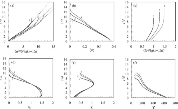
Fig. 2.Computed profiles of relevant nondimensional ensemble-averaged quantities in the transport layer. (a) Velocity of the granular con-stituent, calculated (——) and power-law adjustment (- - - - -); (b) solid fraction; (c) granular temperature; (d) parameter<; (e) parameterS and (f) parameterY. Simulations 1, 2, and 3 correspond toY= 1.74,Y&2.49, andY&3.07, respectively, whereY¼u2
=
Situated above the particles crests, the interfacial layer is dominated by Reynolds stresses. However, form-induced stresses are seen to subsist (Aberle 2006; Aberle et al. 2008; Pokrajac et al. 2008; Ferreira et al. 2009) and, in the presence of sediment transport, drag on moving particles represents a sink in the equation of conservation of momen-tum of the fluid constituent.
For computational purposes, the ensemble of layersAand
B constitutes layer (2) whose thickness is ksT (Fig. 1), termed roughness layer, in the absence of sediment transport (Nikora et al. 2001), or bedload layer, in its presence. It will be assumed that the saltation height is approximately equal to the thickness of the region directly influenced by the bed elements and sediment transport.
The overlapping of the inner and outer flow regions is termed layer C in Fig. 1. Reynolds stresses are dominant and the nondimensional shear rateffiffiffiffiffiffiffiffiffiffiffiffiffiffi ðz=uÞdhui=dz, whereu¼
tb=rðwÞ p
and tb is the bed shear stress, exhibits complete
similarity with respect to inner and outer scales if sediment transport is low or inexistent, allowing for the derivation of the logarithmic law for the vertical profile of the longitudi-nal velocity (Barenblatt 1996; Ferreira 2005; Koll 2006). Self-similarity breaks down at higher transport rates but the profiles, influenced by the magnitude of sediment transport and by the bed surface mixture, should remain logarithmic (Ferreira et al. 2008, 2009).
If the relative submersion is not high, it is still possible to observe the existence of a region, above the crests of the pro-truding particles, where a logarithmic law still holds, provided that the parameters of the low-log are modified (Dittrich and Koll 1997; Franca and Lemmin 2004; Koll 2006; Franca et al. 2008) or if kinematic scales other thatu*are used.
Layer D corresponds to the upper layer of the outer re-gion, where free-surface effects should be included in the equation for the longitudinal velocity profile and where the stress tensor is composed of Reynolds stresses only. Layers
CandDare merged in computational layer (1).
For computational purposes, the bed elevation, Zb, is de-fined as the elevation of the plane of the lowest troughs in a referential whose vertical coordinate has a arbitrary origin. If the bed is composed of a poorly sorted sediment mixture, further computational layers must be introduced below the elevation of the lowest troughs. Computational layer (3) is the mixing layer, after Hirano (1971), where sediment ex-change between the substratum, layer (4), and the bedload
layer (2) occurs. The introduction of layer (3) allows for ex-plicit consideration of vertical sediment fluxes. Acting like a filter, this layer controls both the incoming fractions to the bed and the outgoing fractions to the transport layer (Hirano 1971; Cui et al. 1996). The substratum is a passive layer where sediments are stored. For computational purposes, this may be discretized in layers parallel to the plane of the bed.
2.2. Flow structure of immature debris flows
These flows feature a more complex interaction between moving particles, bed, and fluid. Simple relations for the stress tensor are not possible without a good number of approxima-tions and hypothesis (Savage and Hutter 1989; Jenkins and Richman 1985; Jenkins and Hanes 1998; Po¨schel et al. 2002). Generalizing Yalin’s (1971, 1977) analysis of the fundamental variables for the study of two-phase phenomena, it is argued, after Iverson (1997) and Ferreira (2005), that stresses in a dense, poorly sorted mixture of fluid and cohesionless sediment particles obey the functional dimensional relation
½1 T ¼f
z;e;4;hni;d;hdu=dzi;hQi;rðwÞ;rðgÞ;R;mðwÞ
wherez=hb–zis the normal (perpendicular to the plane of the bed) coordinate measured from the top of the transport layer,hbis the thickness of the transport layer, zis the nor-mal coordinate (measured from the bed), e is the normal coefficient of restitution, 4 is the dynamic internal friction angle, hniis the solid fraction, dis the representative grain diameter, hdu=dzi is the shear rate, hQi is the granular temperature (defined as the sum of the square of the grain velocity fluctuations, measures the state of agitation of the granular medium, Ogawa (1978), r(w) and r(g) are the fluid
and particle densities, respectively, R = g(r(g) –r(w)) is the
submerged weight of particles per unit volume and m(w) is
the fluid viscosity. If the solid fraction near the bed is high ( >&20%), a first hypothesis, included in relation shown in eq. [1], is that turbulent stresses are negligible vis-a-vis other type of stresses, namely those originated in the granu-lar phase (Iverson 1997).
Choosing d, hdu=dzi, and R as basic variables, applying the Vaschy-Buckingham theorem, and combining the result-ing nondimensional parameters, one obtains
½2 T
rðwÞd2hdu=dzi2¼
Y z
d;e;4;hni;<;s;S;Y
sediment. Parameters<,S, andYcan be employed to char-acterize the structure of the transport layer. They account for the influence of (i) binary collisions as a means to trans-fer momentum between moving particles and source of col-lisional stresses (Jenkins and Savage 1983; Lun et al. 1984; Jenkins and Richman 1985, 1988), (ii) streaming motion, i.e., particle velocity fluctuations in the interval between collisions or other interaction with other particles, source of streaming stresses (Jenkins and Richman 1988; Campbell 1989), (iii) enduring frictional contacts among particles and particles and the bed, source of frictional stresses (Savage 1979; Savage and Hutter 1989), and (iv) fluid viscosity (Ar-manini et al. 2005; Ferreira 2005).
Parameter< ¼dhdu=dzihQi1=2 (Savage and Jeffrey 1981;
Lun et al. 1984), the ‘‘shear efficiency number’’ (Ferreira 2005), is a measure of the correlation between the genera-tion of collisional stresses and the state of agitagenera-tion of a granular flowing system. It can also be interpreted as a measure of the efficiency of the shear work in generating a particular state of agitation, measured by the granular tem-perature. Parameter S¼rðwÞd2hdu=dzi2=ðRhnizÞ, the Savage
number (Savage and Hutter 1989), acquired relevance after Savage (1979), in the context of the study of the flow of granular material obeying a Coulomb–Mohr rheology. It represents the ratio of collisional stresses to frictional stresses. The former is identified by the quadratic depend-ence on the shear rate and the later is indirectly represented by the submerged weight, per unit bed area, of granular ma-terial. Parameter Y¼Rhniztanð4Þ=mðwÞhdu=dzi (Iverson 1997) expresses the relation between stresses born by long-term frictional interactions and fluid viscous stresses.
Ferreira (2005), following Jenkins and Hanes (1998), per-formed a theoretical study of the transport layer of a sloping bed with intense transport. Considering a two-dimensional (2-D) vertical flow of a dense mixture of fluid and sediment, the equations of conservation of momentum of the fluid and of the granular phase and the equation of conservation of the particle fluctuating energy were solved numerically sub-jected to appropriate boundary conditions. A detailed ac-count of the solution procedure and of the boundary conditions can be found in Ferreira (2008). The most impor-tant aspects can be summarized as follows. Atz= 0, (i) the granular pressure is the submerged weight, per unit area, of the volume of granular material and the granular shear stresses are frictional and equal to the granular pressure mul-tiplied by tan(4b), where 4b is the friction angle at the bed;
(ii) the no-slip condition applies to fluid and granular veloc-ities; (iii) the solid fraction is equal to the reciprocal of the porosity; (iv) the granular temperature is calculated from a granular equation of state (Lun et al. 1984; Jenkins and Richman 1985, 1988), given the granular pressure; and (v) the flux of fluctuating energy follows from a modification of the solution of Jenkins and Askari (1991) across the bot-tom boundary to account for frictional effects (Ferreira 2005). Atz= hb, (i) the flux of fluctuating energy, the solid
fraction, and the granular pressure are zero. The shooting method employed to solve the system requires that hb and
e(gw), the submerged coefficient of restitution, are unknown
parameters (Ascher et al. 1995). The constitutive equations for the granular stress tensor are derived from the dense limit of the kinetic theory of gases (Chapman and Cowling 1970), introducing energy dissipation by inelastic collisions
(Jenkins and Richman 1985, 1988) and due to fluid viscosity (Ferreira 2005). Selected results of the numerical simulations as well as the profiles of<,S, andY, are displayed in Fig. 2.
Low values of<are typical of diluted systems (low-solid fraction), where streaming stresses are dominant; values of the order of the unity signify that collisional stresses prevail over streaming stresses. It is seen in Fig. 2dthat<increases towards the bed, where a given shear rate (Fig. 2a) produces a small amount of granular temperature (Fig. 2c); on the con-trary, in the diluted upper regions of the transport layer (Fig. 2b), the same shear rate is likely to produce an intense state of agitation. Low values of S are associated to a pre-dominance of frictional stresses over collisional. Observing Fig. 2e, it is expected that frictional stresses prevail near the bed. Parameter S is O(1), where collisional stresses domi-nate. Large / (small) values ofYsignal the preponderance of frictional / (viscous) stresses over viscous / (frictional). Fig-ure 2f shows that, at the bottom of the transport layer, fric-tional stresses are more important than viscous. However, in the core of the transport layer, the influence of fluid viscosity is never negligible as seen by the fast decrease ofYwithz.
Figure 3 synthesizes the information relative to the struc-ture of stress-production mechanisms. An idealization of the mean (time-averaged) velocity profile is also shown. Granular frictional stresses are dominant near the bed, in the frictional layer (A). Above, the core of the transport layer, is designated by collisional layer (B), where collisional stresses are domi-nant but viscous stresses play a nonnegligible role (Ferreira 2005). At the top of the transport layer, a transition layer ex-ists (C), where streaming stresses dominate over collisional. For a small quantity of particles moving in a turbulent flow of a viscous fluid, as is the case in the upper region of layerC, it is assumed that the degree of freedom between the fluid mo-tion and the particle momo-tion is small and that streaming stresses are small compared with Reynolds stresses.
For computational purposes, layer (1) includes the upper-most flow layer (Din Fig. 3) and the transitional layerC. In these layers, the velocity profile is approximately logarith-mic and dominated by turbulent stresses. Computational layer (2), identifiable with the transport layer, is composed of layers A and B. As discussed in Sect.3.2.1, the velocity profile is well adjusted to a power law.
Computational layer (3) corresponds to the bed, where grain movement is reduced to its state of agitation. For com-putational purposes, the bed elevation, relative to an arbi-trary horizontal plane, is defined as the bottom boundary of the frictional layer A, i.e., the elevation of the uppermost layer of particles that have no longitudinal movement.
2.3 Multiple-layer modelling: Equations of conservation
Multiple-layer conceptual approaches interpret flow varia-bles as depth-averaged quantities, integrated over layer thicknesses. This approach achieves a balance between com-putational simplicity of depth-averaged models and
phenom-enological complexity of three-dimensional (3-D)
descriptions by addressing explicitly vertical exchange proc-esses between layers.
and (ii) are susceptible to be described by an equivalent con-tinuum of granular material and fluid mixture.
Conservation equations for the layered systems described in the previous sections can be derived by depth integrating the two-dimensional vertical (2-DV) conservation equations for each of the phases within the continuum hypothesis (de-tails in Ferreira 2005). In one-dimensional (1-D) cases, the overall mass conservation equation is
½3 @tðhþZbÞ þ@xðuhÞ ¼0
where uis the depth-averaged flow velocity, Zb is the bed elevation, and t and x are the time and space coordinates, respectively. The sediment mass conservation equations in layer (2) are
½4 @t
b Cðk2Þhb
þ@xðCbkubhbÞ f
net
sk3;2¼0
whereubis the velocity of layer (2),fnets
k3;2 is the net rate of sediment mass of size fraction k exchanged between layers (2) and (3), Cbðk2Þ is the depth-averaged concentration of size fraction k in (2) andCbk is the flux-averaged concentration of size fractionkin (2).
In layer (3), the mixing layer, conservation of each size fraction in the mixing layer is
½5 ð1pÞ@tðLaFkÞ þfnetsk3;2f
net
sk4;3¼0
wherepis the bed porosity, Lais the thickness of the mix-ing layer, Fk is the percentage of the size fraction k in the mixing layer, and fnets
k is the net rate of sediment mass of size fractionkexchanged between the mixing layer and the substratum. The mass conservation equation in the bed is
½6 ð1pÞ@tðZbÞ þfnets3;2¼0
wherefnets3;2 is the net rate of sediment mass exchanged be-tween layers (2) and (3). It is implied by eqs. [4], [5], and [6] that fnet
3;2 is the net rate of mass exchanged between
layers (2) and (3) and thatfnet3;2¼fsnet3;2=ð1pÞ.
The equation of conservation of momentum is obtained by summing the corresponding momentum equations of each of the layers. It is implicit that the velocity and the shear stress profiles are continuous across the boundary be-tween layers (1) and (2) (refer to Ferreira 2005, Sect. 3 for details). The result is
½7 @tðrmuhÞ þ@x
rbub2hbþrðwÞuw2hw
þ1
2g@x
rðwÞhw2þrðwÞhwhbþ2rbhb2
¼ grbhbþrðwÞhw
@xðZbÞ t3;2
wherehw= h–hbis the thickness of layer (1),uw= (uh–ubhb)/(h–hb) is the velocity of layer (1),rm=r(w)[1 + (s– 1)C]
is the mean flow density, rb = r(w) [1 + (s –1)C
b] is the density of layer (2), C = Cbubhb/(uh) is the mean flux-averaged
concentration of sediment, Cb is the flux-averaged sediment concentration in (2) andt3;2tb is the force per unit area
be-tween layers (2) and (3) (bed shear stress).
The system of partial differential eqs. [3–7] has 3 + n+ (n–1) unknowns, wheren is the number of size fractions in the bed. These unknowns are the flow elevationZs=h+Zb, the mass discharge per unit widthRm =rmuh,Zb,Cbk fork= 1,. . ., n, andFkfork= 1,. . .,n– 1, where, naturally,
X
k
Fk¼1.
The next section is dedicated to present the closure equations for hb,ub,Cb,La,fnets
k3;2, andf net
sk that complete the concep-tual models.
3. Conceptual models for the transport layer
3.1. Coarse-bedded streams with weak sediment transport
3.1.1. Thickness and velocity of the bedload layer
It is assumed that the thickness of the bedload layer is the distance between the elevation of maximum of the zenith of the saltation paths and the elevation of the troughs of the bed. Modifying Owen’s (1964) analysis, it is considered that the max-imum potential energy of a saltating particle equals its kinetic energy at entrainment minus the work of the drag force during its vertical excursion plus (or minus, if the particle is faster than the surrounding flow) the work of the lift force:
½8 rðwÞðs1Þd3
mCVgzmax ¼
1 2r
ðwÞsd3
mCVw20
1 2r
ðwÞd2
mC1CDw20zmax þ
1 2r
ðwÞd2 mC1CLh
uðwÞuðgÞjuðwÞuðgÞjiz max
wherezmaxis the height above the rest point that is attained by the particle performing the higher jumps,dmis the diameter of the
particle that performs the higher jumps,CVis the ratio of the actual particle volume to the volume of a sphere whose diameter is dm,C11is the ratio of the larger particle axis todm,w0is the initial vertical particle velocity, andhuðwÞuðgÞ
juðwÞuðgÞjiis the average lag velocity between the particle (superscript g) and the surrounding fluid (superscript w).
It is implicit in eq. [8] that the work of drag in the longitudinal direction affects the jump length, not the jump height. Considering the particle that attains the highest position above the bed is entrained at an elevation of d90 from the lowest trough and both the particle and the fluid velocities are expressed as huðwÞuðgÞjuðwÞuðgÞji ¼m
uðu2u2refÞ and w2
0¼mwðu2u2refÞ, we obtain
½9 hb
d90
¼1þ
1
2sðdm=d90ÞCVmwðY50YrefÞ
ðdm=d90ÞCVþ 12C1CDmw12C1CLmu
Fig. 5.Time- and ensemble-averaged longitudinal fluid velocity profiles (*) for four uniform, capacity, laboratory tests. (a)Fr= 0.40, Y50= 0.021,kþs ¼ksu=n¼153; (b)Fr= 0.43,Y50= 0.026,kþs ¼157; (c)Fr= 0.60,Y50= 0.039,k
þ
s ¼227; (d)Fr= 0.61,Y50= 0.050,
kþs ¼346. Full line indicates eq. [11]. Dotted line indicates the logarithmic law.
Fig. 6.Partition of the flow energy through the different scales of a wavelet multi-level decomposition; results obtained at one point within the boundary layer of a gravel-bedded stream (after Franca 2005, Sect. 3.6).
where Y50¼u2=ðgðs1Þd50Þis the Shields parameter
com-puted with the median diameterd50,Yrefis a reference value of Shields’ parameter such thatY50< Yref)hb¼d90. From
the shape data presented in Ferreira et al. (2007), CV= 1.0,
C1 = 1.2. Laboratory data, presented in Ferreira (2005), ob-tained withdm = 2.3 mm andd90 &5.0 mm, allows one to compute uref¼0:029, Yref = 0.022, and mu 10 (see also
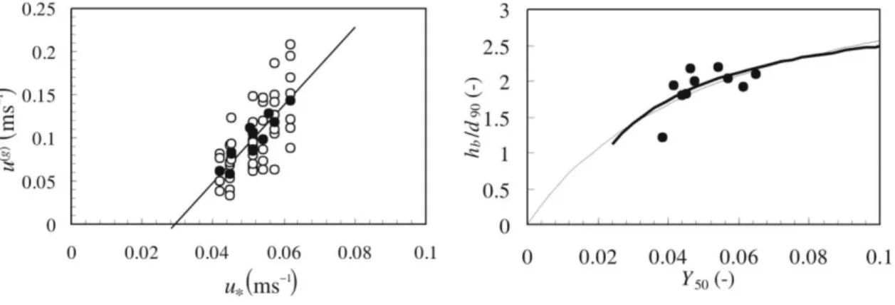
Figs. 4a and 5). Considering that CD = 0.4 and CL = 0.2 (Ferreira et al. 2007), we found that the angle at which the particle leaves the bed and its modulus by minimizing the mean square error between the computed values and the va-lues drawn from the laboratory data of Ferreira (2005). The experimental results and fitted eq. [9] are displayed in Fig. 4b.
Fig. 7.(a) Three-dimentional (3-D) reconstruction of a bursting cycle, sampled through wavelet-based multilevel decomposition (time nor-malized by event duration and velocities nornor-malized by difference of the maximum and minimum event velocities detected for the most energetic scale, details in Franca 2005, Section 3.6); points 1 and 5 are the beginning and end of the cycle. (b) Distribution of the time period between consecutive events (after Franca and Lemmin 2006).
The fitting procedure led tomw= 47.1 and an initial flight angle of 458, which means that the horizontal velocity at the moment of entrainment is of the order of magnitude of 10u*, which is plausible. For computational purposes, it is desir-able that hb = 0 whenY50 = 0. For that reason, the approxi-mate expressionhb/d90= 73Y50/(1 + 18.5Y50), also displayed
in Fig. 4b, is used for small values of Y50.
The velocity of layer (2) is a composition of the mean ve-locities of the grains moving as bedload (ucb) and the mean velocity of the fluid (uwb). The path- and ensemble-averaged velocity of the particles travelling as bedload (shown in Fig. 4afor gravel and sand-size fractions) reveals that single linear function ofu* applies to all size fractions (Ferreira et
al. 2006a). The latter is
½10 ucb¼4:5ðuurefÞ
where uref ¼0:029 m3s–1 is deduced from the coefficients
of the linear regression. Equation [10] is comparable to that proposed by Nin˜o et al. (1994).
As for the fluid velocity, the data of Ferreira (2005), al-lows one to characterize profiles of the longitudinal velocity. Four typical profiles, representing the upper parts of the bedload layer, the logarithmic layer, and the lower parts of
the free-surface layer, are shown in Fig. 5. They are a result of a time and an ensemble averaging process: four independ-ent time-averaged profiles are considered for the ensemble average. Nikora et al. (2001) proposed that the time- and space-averaged velocity profile in the roughness layer should be linear in zl/ks wherezl= z –D,ks= ksT –D, ksT
is the characteristic scale of the roughness elements (Fig. 1), and D is the displacement height (see Ferreira et al. 2009 for a discussion of the value of these parameters). However, analysis of the experimental data reveals that
½11 uðzÞ
u
¼m1zl ks
þb1
where m1 = 6.2 andb1 = 3.4 for the particular mixtures of
the laboratorial tests.
It is noted that eq. [11] predicts a slip velocity at z= D, i.e., the velocity in the bedload layer cannot be linear throughout its entire thickness. Near the troughs, a zone do-minated by flow separation, the time- and space-averaged velocity is probably dependent on the arrangement of the bed surface, rendering m1 and b1 dependent on flow varia-bles and on the bed mixture.
The integration of eq. [11] results in uwb =u*{m1/2 + b1} if it is assumed that hb & ksT –D. The depth-averaged ve-locity of the fluid in the bedload layer becomes uwb= 6.5u*. Finally, the velocity in the bedload layer is (refer to Ferreira 2005 for details)
½12 ub ¼uwbCb ð2Þ
ðuwbucbÞ
where the depth-averaged sediment concentration is b
Cð2Þ2Cb for low to moderate concentrations (Ferreira et
al. 2006a).
3.1.2. Near-bed organised turbulence and detection of sediment driving coherent structures
Intermittent organized motion within the boundary layer, like bursting phenomena, is intrinsically related to transport processes. The characterization of bursting phenomena was put forward by Grass (1971), Nakagawa and Nezu (1977), among others. Recently, experimental results on coherent motion in gravel-bedded flows have been shown by Franca
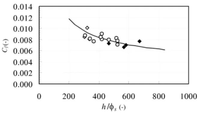
Fig. 9.Friction factor defined as Cf= (u*/u)2. Equation [15] (——) is superimposed to laboratorial data: mobile sand–gravel bedded tests (^); armoured sand–gravel bedded tests (^), and mobile and sub-threshold gravel bedded tests (*).
Fig. 10.Thickness of the transport layer as a function of Shields parameter. Sensitivity analysis to the characteristics of the sediment grains. The four types of granular material used by Sumer et al. (1996), were plastic (d= 0.003 m,s= 1.27,e= 0.75 andd= 0.0026 m,s= 1.14,e= 0.75), acrylic (d= 0.0006 m,s= 1.13,e= 0.75) and sand (d= 0.00013 m,s= 2.67,e= 0.8);n0= 0.6; tan(4b) = 0.4;q= 1.0 m2/s. Circles (*) stand for Sumer et al. data.
and Lemmin (2006) from a natural armoured river and by Ferreira et al. (2002) from flow over gravel-sand beds with bedload.
The assessment of the momentum generated by coherent structures needs to account for the duration (time scale) of their cycle. The application of wavelets is suitable to iden-tify and analyze coherent structures in the boundary layer of geophysical flows (Foufoula-Georgiou and Kumar 1994 and others). Wavelet decomposition allows one to evaluate the energy partition throughout the scales present in the instan-taneous velocity signal; Fig. 6 is based on results obtained in one point within the boundary layer of a gravel-bedded stream (Franca 2005, section 3.6).
Franca and Lemmin (2006) applied an algorithm of detec-tion and reconstrucdetec-tion of coherent structures based on the wavelet multiresolution analysis to the most energetic scale seen in Fig. 6 (DT = 0.43 s), allowing the reconstruction of a bursting cycle (Fig. 7a) with a sweep and an ejection scal-ing both withDT. For the positive detection of an event, the comparison of the instantaneous shear stress relative ampli-tude with threshold value QH > 5 was used, where QH is evaluated locally and corresponds to the ratio between the reconstructed shear series within the analysed wavelet scale and its mean value. From the distribution of the time period between the occurrence of the bursting cycle (T), it was found that the observed bursting packets are independent. The intermittency character of the event is represented byT
which had an extreme-type statistical distribution (Fig. 7b), where the most probable value correspond to T = 2 s. In this case, the persistency factor DT/T,a measure of the mo-mentum input from the detected structures, is 0.22.
3.1.3. Equilibrium bedload discharge
The hypothesis that entrainment and transport of sediment particles are related directly to organised turbulence may be traced to the work of Sutherland (1967). Prior to the concept of coherent turbulent events, he performed a landmark study built around the idea that sediment is entrained when a mass of fluid impinges on the bed. In a turbulent flow, the mass of fluid takes the form of a sweep event, which promotes its entrainment by increasing locally the hydrodynamic ac-tions upon the particles past their critical stability values. . This description embodies the concept of event-driven bed-load transport. The event-driven sediment transport model developed here is based on those developed by Hogg et al. (1996) and Ferreira (2005), the latter for granulometric mix-tures.
It is considered that under small mean shear, the ratio of the bedload concentration during an impinging event to (Y –Yc)3/2 is a constant (where Y ¼rðwÞu2
=
gðs1Þd
is Shields’ parameter and Yc is a critical Shields’ parameter). Under this assumption, the bedload discharge is propor-tional to Yb, b > 3/2, a fact experimentally observed by Wilcock et al. (2001) among others. Under this hypothesis one has
½13 Ek=ðFkAIVHkÞ ðYkYckÞ3=2
¼c
where Ek is the volume of sediment of size fraction k
en-trained during a sweep event,AIVis the area of influence of
the sweep event per unit width, Hk is the thickness of the
erodible layer for size fraction k, and c is a constant. The group FkAIVHk is the volume of sediment and voids from
which the sweep event can extract sediment whereas the group Ek/(FkAIVHk) can be interpreted as the sediment con-centration that can be locally generated by a sweep event if all particles were of sizek. Obviously, by ‘‘sweep event’’ it is meant a statistically representative event, for instance, the expected value of its distribution. Using Taylors’ frozen tur-bulence hypothesis, the area of influence of the event can be written as AIV = DT u0, where u0 is the time- and space-averaged fluid velocity at the level of the crests of the bed elements. An estimation for u0 comes from eq. [11], u0 =
5.2u*. The thickness of the erodible layer is a fraction of the thickness of the mixing layer. For the largest grains in the bed, Hk is the full thickness of this layer in the sense
that their entrainment implies the removal of a volume of bed material whose height is equal to the thickness of the mixing layer. The entrainment of smaller represents the re-moval of a thinner equivalent layer of bed material. To ac-count for this hiding effect, a distribution function Wk,
approximated bydk/dmax, where dmaxis the sieving diameter
of the larger particle found in the bed surface samples, is introduced. If the thickness of the mixing layer isLa= 3d50,
then Hk = 3d50Wk. Substituting these definitions and
esti-mates in eq. [13], the volume of sediment of size fractionk
entrained by each sweep event is obtained. To know the bedload discharge, it is necessary to know the frequency of the events. Thus, the bedload discharge for each size frac-tion k, q
sbk, is obtained by dividing the respective volume by the period,T, of the representative sweep event.
Employing the ratio DT/T = 0.22 previously evaluated in Sect. 3.1.2, eq. [13] becomes
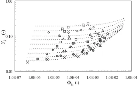
½14 Fk¼3:56cWk d50
dk ðYkYckÞ 3 2Y
1 2 k
where Fk¼qsbk=
gdkðs1Þ 1 2
dkFk
. The values of c =
1.00 and Yck were determined empirically using Ferreira’s
(2005) laboratory data for a gravel–sand mixture (details in Ferreira et al. 2007 about Yck). The graphical expression of
eq. [14] can be seen in Fig. 8 along with the laboratory data.
3.1.4. Flow resistance
The friction factor, defined here asCf= (u*/u)2, in gravel–
sand bedded streams with weak sediment transport can be derived from the logarithmic velocity profile plus eq. [11]. One obtains
½15 Cf ¼ 2:5ln 0:22
h zs
2
where the roughness length is zs = (ksT – D)e-kB, B is the
constant in the logarithmic law, and k = 0.41 is the von Ka´rma´n constant. The parameters ksT and B were fitted from experimental data with a procedure explained in Fer-reira et al. (2008a). Equation [15] was superimposed to la-boratorial values ofCf, as shown in Fig. 9.
It is underlined that the value of u* in the definition ofCf
includes shear stresses and form drag at the bed. The experi-mental values ofCfwere calculated fromCf= –gRh@x(Zb)/u2,
whereRhis the bed hydraulic radius, determined with a
3.1.5. Vertical fluxes and mixing layer
The vertical flux between the substratum and the mixing layer is
½16 fnetsk4;3¼ ð1pÞfIk@tðZbÞ
The composition of the sediment transferred between these layers is controlled by the transfer functionfIk, the proportion of the size fraction k at the interface (Toro-Escobar et al. 1996). In an aggradational process, the formula of Cui et al. (1996) is used: fIk ¼bIpkþ ð1bIÞFk, where pk stands for
the composition of the bedload and bI should be calibrated from existing data (Cui et al. 1996 used 0.7, Ferreira 2005, used 0.3). If erosion is dominant, Hirano’s (Hirano 1971) concept holds andfIk ¼fk, wherefkis the composition of the substrate. Note thatbI= 0.0 should not be used because it is incompatible with downstream fining (Parker 1991).
The hypothesis that the flux between the mixing layer and the bedload layer is proportional to the imbalance between capacity and actual bedload discharge is pursued in this work (time and space lag effects). Thus, it can be written
½17 fnet3;2¼ q
sb Cbkubhb L
whereLis a geometric scale associated to the length neces-sary for the attenuation of a given imbalance. Expressions for bedload are given by Phillips and Sutherland (1989) among others but, in general,Lmust be calibrated with ex-perimental data.
3.2. Immature debris flows
3.2.1. Thickness and velocity of the transport layer
An analysis of the numerical results shown in section 2.2, especially Fig. 2, allows one to determine an equation for the velocity of the mixture in layer (2). A good fit to the re-sults in Fig. 2ais
½18 uðzÞ
u
¼2:1 G
Y
3=4 z
h
3=4
adapted from Sumer et al. (1996), where G = h/d. The re-sulting equation for the depth-averaged velocity is
½19 ub¼uð1:2ÞðG=YÞ3=4ðhb=hÞ3=4
Depth-averaging the equation of conservation of the fluc-tuating energy, Ferreira (2005) obtained an algebraic relation for the thickness of the transport layer, graphically expressed in Fig. 10 along with the experimental results of Sumer et al. (1996).
It is apparent that hb/dis not a direct function of the pa-rameters that characterize the transported, namely, the resti-tution coefficient and the internal friction angle at the bed as the lines corresponding to different sediment are essentially superimposed in Fig. 10. The influence of the density and the diameter is felt only through Shields parameter. The thickness of the transport layer can be approximated by
½20 hb
d ¼1:7þ5:5Y
3.2.2. Equilibrium concentrations and vertical fluxes The existence of a frictional layer, across which the shear stress may vary, allowed Ferreira (2005), to determine the mass flux between the bed and the transport layer and the depth-averaged sediment concentration in the latter. The in-tegration of the equation of conservation of momentum in the vertical direction over the frictional layer renders
½21 @tðZbÞ ¼fnet3;2 ¼
grðwÞðs1Þtanð4bÞ ubðrbuxÞjz¼Zf
ðqsbqsbÞ
whereZf is the elevation of boundary between the frictional and collisional layers (layers A and B in Fig. 3), qsb = Cbubhb is the volumetric bedload discharge and
q
sb ¼Cbubhb is the equilibrium volumetric bedload
dis-charge. The equilibrium concentration is derived from the following considerations: (i) by definition, one has
Tðz¼ZbÞ ¼tbrðwÞCf u2, where Cf = (u*/u)2 is the
fric-tion factor of the overall flow; (ii) in a steady, equilibrium flow one has Tðz¼ZbÞ ¼grðwÞðs1ÞCbhbtanð4bÞ, where Cb is the equilibrium concentration; hence, the equilibrium concentration is
½22 Cb ¼ Cf u
2
gðs1Þtanð4bÞhb
3.2.3. Flow resistance
The results of Sumer et al. (1996) allows one for the com-putation of the friction factor. It is apparent in Fig. 11 that the bed shear stress can be adequately described by tb rðwÞCf u2 provided that the friction coefficient is
½23 Cf ¼0:02
h d
1=2 w s
u 1=2
for low values of u*/ws, wherews is the fall velocity.
Equa-tion [23] is plotted against the data of Sumer et al. (1996) in Fig. 11 and it is shown to be applicable to the most com-mon flow regime, characterized by moderate to large values of h/d. A second flow regime, for low values of h/d, is de-tected (dashed lines in Fig. 11) but its characterization is out of the scope of the present work.
4. Solutions
4.1. Morphological and textural evolution of gravel- and sand-bedded streams
The results of the model described in Sections 2.3 and 3.1 were compared with laboratory data from a set of experi-mental tests of aggradation and degradation, performed at the Laboratory of Fluid Mechanics, University of Aberdeen in a 12 m long, 40 cm wide, glass-walled recirculating tilt-ing flume. Details of facilities, instrumentation and experi-mental procedures can be found in Ferreira (2005). The mathematical reproduction of two laboratorial tests is shown herein. The most relevant initial and boundary conditions of the tests are shown in Table 1.
water depth measured in the recirculation stage constitute the initial conditions for the mathematical model. Sediment recirculation was then disconnected and the bed evolved into an armoured bed. The results of the model can be seen in Figs. 12a — time evolution of bed elevation and water depth, Fig. 13a — time evolution of the bedload, and Fig. 14a— composition of the final bed surface.
The initial conditions of test DA1 are the final, armoured stage of test D1. The sediment discharge, the water depth and the bed surface composition were variables that changed the most. The bed slope was not affected significantly, which is indicative of the protective role of the coarser sedi-ment in the bed. The boundary conditions for test DA1 con-sist of strong sediment overfeeding at the upstream end. Overfeeding was imposed by means of a conveyor belt loaded with sediment with the composition of the bed sub-strate. The results of the numerical simulation can be seen in Figs. 12b, 13b, and 14b.
The solution procedure is based on a finite-difference ex-plicit discretization of eqs. [3]–[7]. The discretization
scheme closely follows MacCormack’s (MacCormack
1969). Being a second-order scheme, spurious oscillations near discontinuities will occur. To achieve a monotone solu-tion at discontinuities, a TVD version is used in which the TVD step incorporates the minmod flux limiter (see Ferreira 2005). Jameson’s artificial viscosity is used in the equations of conservation of sediment mass (for a discussion of the scheme see Hirsch 1990). The mesh size was Dx = 0.05 m for all tests.
In what concerns test D1, the model slightly overesti-mated the bed degradation while reproducing the water depth correctly (Fig. 12a). The predicted bed composition was only slightly coarser that the measured one (Fig. 14a). It is concluded that the flow resistance is well modelled but that the phenomenon of hiding is not properly addressed in the formulation of Yck in eq. [14]. The total bedload
dis-charge is well captured by the model. The evolution of the bedload is essentially correct, but the composition is not well predicted (Fig. 13a). This points to the necessity on further experimental work in the formulations for Wk and Yckin eq. [14].
Since the imposed discharge is of the order of magnitude of the transport capacity, the aggradation process in test DA1 is not in the form of a sharp-edged wave (Fig. 12b), a feature well captured by the numerical model. The simulated total bedload discharge does not reflect the measured high variability (Fig. 13b). At high times, the bedload discharge appears overestimated as well as the bed elevation at x = 9.0. This might indicate that the characteristic scale of bed-load propagation, greatly dependant on the formulations for
ub, hb and, especially, fnet3;2, may be overestimated in the model. The final computed bed composition, with bI = 0.3,
is finer than the registered one, that is, the initial prearm-oured bed is attained faster than what was observed (Fig. 14b). This corroborates the hypothesis that the mor-phological characteristic velocities are overestimated in the model. A sensitivity analysis to the values of bI may help in understanding if the root of the problem lies on the mix-ing layer idealization or on the specific parameters em-ployed to characterize it.
4.2. Morphological evolution of geomorphic flows featuring immature debris flow
Modelling geomorphic flows requires the application of models, developed within the shallow-flow paradigm, for which the closure equations express flow and sediment dy-namics and morphology characteristic of immature debris flows (see Sect. 3.2).
To evaluate the capability of the model to deal with flows observed in nature, the case study of the Ha! Ha! River 1996 dam-break was chosen. Severe rainstorms scourged southern Que´bec, Canada, between the 18th and the 21st of July 1996. Because of the overtopping and sequent failure of an earthfill dyke, Ha! Ha! River experienced a significant in-crease in the peak flood discharge. The dam-break wave, superimposed the hydrologic flood, provoked massive geo-morphic impacts in the downstream valley (Lapointe et al. 1998; Capart et al. 2007).
It should be highlighted that the simulation of this ex-treme flood event represents a highly demanding computa-tional test. Firstly, because the morphologic impacts were unusually pronounced (erosion depths of 20 m and deposi-tion layers of 10 m were registered), which constitutes a challenging test for the underlying conceptual model. For the numerical solution procedure, difficulties arise because of the complex channel geometry, featuring constrictions and enlargements, chutes, and low-slope reaches. As a re-sult, subcritical and supercritical flow regimes may co-exist in the computational domain at a given time. Moreover, flow singularities such as hydraulic jumps or critical flow points can be created and destroyed during the simulation.
The conservation equations included in the model are a generalization of system eqs. [3]–[7] for nonprismatic chan-nels (Ferreira et al. 2005). It is also considered that sediment transport is near capacity (Leal et al. 2006; Fraccarollo and Capart 2002). The solution procedure is based on MacCor-mack’s (1969) scheme. The TVD algorithm revealed inad-equate to tackle oscillations born from strong momentum sources such as abrupt slope variations (details in Ferreira 2005). Von Neumann’s numerical viscosity was used in its place.
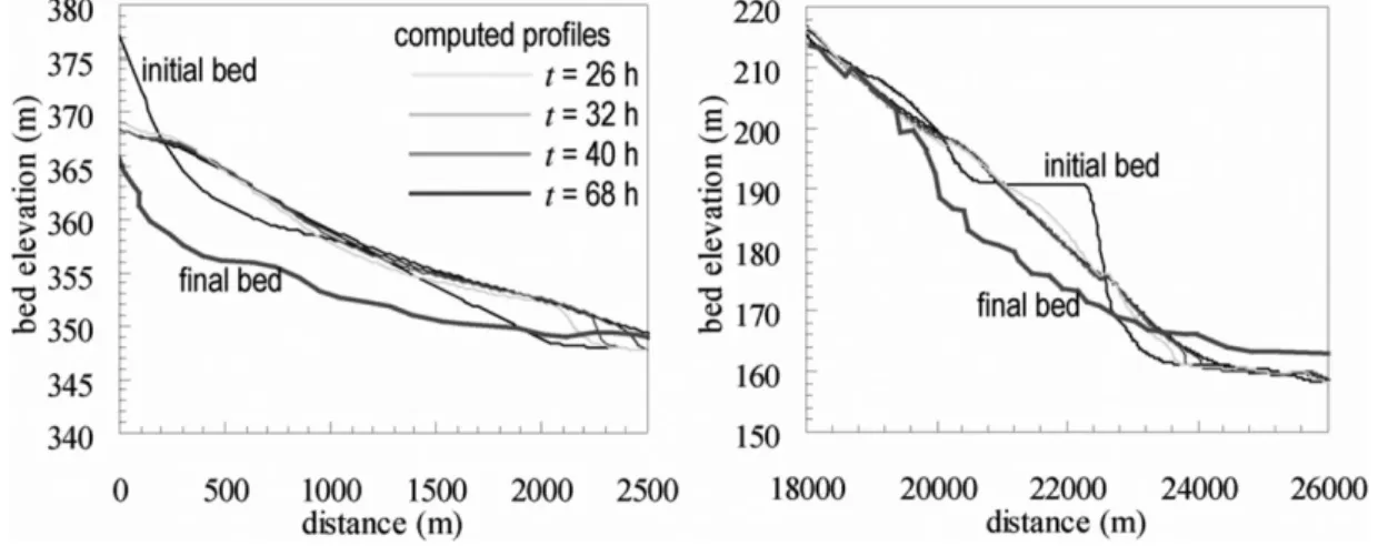
The pre- and post-flood measured bed profiles of the Ha! Ha! River can be seen in Fig. 15, in the reaches where the most important morphologic changes have occurred: down-stream of the failed dyke and at a chute known as Chute a` Perron. The computed bed profiles, corresponding to the ris-ing limb of the discharge hydrograph, can be seen in the same figure.
It was observed that the dyke was eroded completely and so were the sediment deposits below it down to a depth of about 14 m below the initial bed elevation (Fig. 15, left). Massive incision was registered in all convex profiles. In Chute a` Perron, the flood excavated a new channel around the rock outcrop (Lapointe et al. 1998) and severe up-stream-progressing erosion took place (Fig. 15, right). The new bed is 20 m below the old river bed in some places.
for flow variables, i.e., at t = 0 h (details in Ferreira 2005, 2008, or Ferreira et al. 2005).
Most of the hydraulic jumps and sonic points disappear dur-ing the risdur-ing limb of the hydrograph. In the same period, one new sonic point and one new hydraulic jump were created at the transition between fixed and mobile bed reaches (kilo-metre 15). It is noted that the upstream migration of the sonic points is due, as in the case of the knickpoint migration, to the upstream erosion of the point of minimum curvature radius.
The hydraulic jumps identified in Fig. 16, progress in the downstream direction (Leal et al. 2002). This is a conse-quence of the wave structure of system eqs. [3]–[7]: in
mo-bile bed flows, discontinuities cannot be purely
hydrodynamic because the bed elevation or the sediment concentration are dependent variables of the system of con-servation laws (further discussion in Ferreira et al. 2006b). These hydraulic jumps are associated to a discontinuity in the bed elevation that moves necessarily downstream at a slow velocity until eventually disappearing.
5. Conclusions
Fluvial engineering practice benefits from computational tools for which the phenomenological core are conservation and closure equations, i.e., the conceptual model. The later is drawn from the empirical base of the successful research programs in fluvial processes. Proposals for the conceptual models of two fluvial flow typologies are, in this text, pre-sented. These proposals are based on existent empirical knowledge and on research efforts undertaken by the authors in the past ten years. One of the flow types addressed is that of flat coarse-bed rivers. The other corresponds to geomor-phic flows, for which sediment transport is intense, in the form of immature debris flow.
It is argued that both these flows can be idealized as mul-tiple-layered. The conservation equations of both flows can be derived within the continuum shallow-flow paradigm. Furthermore, it is sustained that, in both flow types, sedi-ment transport and flow resistance depend, essentially, on
Table 1.Initial and boundary conditions of gravel-sand bedded tests.
Test Q(m3s–1) h0(m) i0(–) Q
b0(10–3kgs–1) Qb1(10–3kgs–1)
D1 0.0135 0.069 0.0025 1.698 0.0
DA1 0.0135 0.072 0.0024 — 5.21
Note:Q, water discharge;h0, initial water depth;i0, initial slope;Qb0, equilibrium mass sediment discharge;Qb1, sediment
discharge imposed at the upstream reach.
Fig. 12.Time evolution of bed elevation (full symbols) and water depth (open symbols). (a) Test D1; (b) test DA1. Measurements were taken at 3.0 m (&and&), 6.5 m (^and^) and at 9.5 m (*and*) from the inlet.
grain-scale phenomena. Bed forms that scale with the flow depth are absent in the flow description. Indeed, bedload transport rates depend on momentum transfer between fluid and individual grains on the bed, in the case of coarse bedded streams (Section 3.1.3), and on the stability of the frictional sublayer, in the case of debris flows (Section 3.2.2). As for flow resistance, it is seen in Section 3.1.1 and 3.1.4 that u* is much depending on bed texture in coarse bedded streams. In debris flows, flow resistance depends, on collisional and frictional interactions between grains (Sections 3.2 and 3.2.3).
The research efforts presented in Sections 2. and 3. of this text possess strong experimental and theoretical components. Possessing intrinsic empirical value, the results of such re-search are neverthless mainly employed to build coherent conceptual models in this paper, in which both conservation
and closure equations stem from the same theoretical frame-work.
To illustrate the descriptive potential of the proposed conceptual models, numerical solutions were presented and discussed. One of the simulations concerned the morpho-logical and textural evolution of a sand–gravel channel bed, generated in laboratory. Since the closure equations were derived essentially from laboratorial data obtained in the same channel with the same sediment sizes, the simula-tion served the purpose of assessing the internal consistency of the model more than proving its predicting abilities. A second numerical simulation was designed to test the pre-dictive capabilities of the conceptual model for geomorphic flows featuring immature debris flow. The results showed that the model can be used in river engineering contexts, mostly because it requires a little amount of field data.
Fig. 14.Characteristic diameters of the bed surface composition at 6.0 m from the inlet. Simulation results superimposed to initial (- -*- - ) and final (- -^- -) bed data in (a) test D and (b) test DA1. The coordinates are relative to the initial bed for the laboratorial data and for the final bed for the numerical data. From top to bottom characteristic diameters ared90,d80,d70,d50,d30,d20, andd10.
Acknowledgements
The Portuguese Foundation for Science and Technology is acknowledged for the financial support provided through the project PTDC/ECM/65442/2006. The authors thank the two anonymous reviewers whose comments, corrections and sug-gestions helped clarifying many issues in this paper.
References
Aberle, J. 2006. Spatially averaged near-bed flow field over rough armor layers. In River Flow 2006, Lisbon. Taylor and Francis Group, London. Vol. 1, pp. 153–162.
Aberle, J., Koll, K., and Dittrich, A. 2008. Form induced stresses over rough gravel beds. Acta Geophysica, 56(3): 584–600. doi:10.2478/s11600-008-0018-x.
Armanini, A., Capart, H., Fraccarollo, L., and Larcher, M. 2005. Rheological stratification in experimental free-surface flows of granular–liquid mixtures. Journal of Fluid Mechanics, 532: 269–319. doi:10.1017/S0022112005004283.
Ascher, U., Mattheij, R., and Russel, R. 1995. Numerical solution of boundary value problems for ordinary differential equations. SIAM, Philadelphia, Pa.
Bagnold, R.A. 1966. An approach to the sediment transport pro-blem for general physics. Professional Paper 422-I. U.S. Geolo-gical Survey, Washington, D.C.
Barenblatt, G.I. 1996. Scaling, self-similarity and intermediate asymptotics. Cambridge University Press, Cambridge, UK. Campbell, C.S. 1989. The stress tensor for simple shear flows of a
granular material. Journal of Fluid Mechanics, 203: 449–473. doi:10.1017/S0022112089001540.
Capart, H., Spinewine, B., Young, D.L., Zech, Y., Brooks, G.R., Leclerc, M., and Secretan, Y. 2007. The 1996 Lake Ha! Ha!
breakout flood, Que´bec: Test data for geomorphic flood routing methods. Journal of Hydraulic Research,45: 97–109.
Chapman, S., and Cowling, T.G. 1970. The mathematical theory of non-uniform gases. 3rd ed. Cambridge University Press. Chiew, Y.-M., and Parker, G. 1994. Incipient sediment motion on
non-horizontal slopes. Journal of Hydraulic Research, 32(5): 649–660.
Cui, Y., Parker, G., and Paola, C. 1996. Numerical simulation of aggradation and downstream fining. Journal of Hydraulic Re-search,34(2): 185–204.
Dittrich, A., and Koll, K. 1997. Velocity field and resistance of flow over rough surface with large and small relative submer-gence. International Journal of Sediment Research,12(3): 21–33. Einstein, H.A. 1950. The bed load function for sediment transporta-tion in open-channel flows. Bulletin 1026. U.S. Deptartment of Agriculture, Soil Conservation Service.
Ettema, R., and Mutel, C.F. 2004. Hans Albert Einstein: innovation and compromise in formulating sediment transport by rivers. Journal of Hydraulic Engineering, 130(6): 477–487. doi:10. 1061/(ASCE)0733-9429(2004)130:6(477).
Ferreira, R.M.L. 2005. River Morphodynamics and sediment trans-port: Conceptual model and solutions. Ph.D. thesis, Instituto Superior Te´cnico, T.U., Lisbon. pp. 23–41, 57–73, 67–73, 86– 106, 119, 139–141, 148–149, 211–217, 247, 248–249, 254–255, 250–263, 256, 263–278, 279–280, 281, 480–484, 509–510, 510– 523. Available from http://www.civil.ist.utl.pt/~ruif/phdthesis. Ferreira, R.M.L. 2008. Fundamentals of mathematical modelling of
morphodynamic processes: Applicationto geomorphic flows. In Numerical Modelling of Hydrodynamics for Water Resources. Edited by P. Garcı´a Navarro and E. Playa´n. Taylor & Francis. pp. 189–209.
bedded river’s salmonid Habitats. M.Sc. thesis, Instituto Super-ior Te´cnico, TU, Lisbon.
Ferreira, R.M.L., Leal, J.G.A.B., and Cardoso, A.H. 2002. Turbu-lent structures and near-bed sediment transport in open-channel flows. In River Flow 2002, Louvain-la-Neuve. A.A. Balkema. Vol. 1, pp. 553–563.
Ferreira, R.M.L., Leal, J.G.A.B., and Cardoso, A.H. 2005. Mathe-matical modelling of the morphodynamic aspects of the 1996 flood in the Ha! Ha! river.In Proceedings of the XXXI IAHR Congress, Seoul, Theme D. pp. 3434–3445 (CD-ROM). Ferreira, R.M.L., Leal, J.G.A.B., and Cardoso, A.H. 2006a.
Con-ceptual model for the bedload layer of gravel bed streams based on laboratory observations.InRiver Flow 2006, Lisbon. Taylor and Francis Group, London. Vol. 1, pp. 947–956.
Ferreira, R.M.L., Leal, J.G.A.B., and Cardoso, A.H. 2006b. Con-ceptual model for the bedload layer of gravel bed streams based on laboratory observations.InRiver Flow 2006, Lisbon. Taylor and Francis Group, London. Vol. 1, pp. 947–956.
Ferreira, R.M.L., Franca, M.J., and Leal, J.G.A.B. 2007. Laborator-ial and theoretical study of the mobility of gravel and sand mix-tures. In Proceedings of the 5th River, Coastal and Estuarine Morphodynamics, RCEM 2007. Edited by C.M. Dohmen-Jans-sen and S.J.M.H. Hulscher. pp. 531–539.
Ferreira, R.M.L., Franca, M.J., and Leal, J.G.A.B. 2008. Flow re-sistance in open channel flows with mobile hydraulically rough beds. In River Flow 2008. Vol. 1. Edited by Altinakar et al. pp. 385–394.
Ferreira, R.M.L., Ferreira, L.S.M., Ricardo, A.M., and Franca, M.J. 2009. Imposed sand transport on gravel-bedded streams: Impacts on flow variables and consequences for salmonid spawning sites. River Research and Applications, In press. doi:10.1002/rra.1307. Finnigan, J.J. 2000. Turbulence in plant canopies. Annual Review of Fluid Mechanics, 32: 519–571. doi:10.1146/annurev.fluid.32. 1.519.
Foufoula-Georgiou, E., and Kumar, P. 1994. Wavelets in geophy-sics. Academic Press, San Diego, Calif.
Fraccarollo, L., and Capart, H. 2002. Riemann wave description of erosional dam-break flows. Journal of Fluid Mechanics, 461: 183–228. doi:10.1017/S0022112002008455.
Franca, M.J., and Lemmin, U. 2004. A field study of extremely rough, three-dimensional river flow. In Proceedings of the 4th IAHR International Symposium on Environmental Hydraulics. Taylor and Francis Group, London.
Franca, M.J. 2005. A field study of turbulent flows in shallow gravel-bed rivers. Ph.D. thesis, No. 3393, E´ cole Polytechnique Fe´de´rale de Lausanne. Available from http://library.epfl.ch/ theses/?nr=3393.
Franca, M.J., and Lemmin, U. 2006. Detection and reconstruction of coherent structures based on wavelet multiresolution analysis. InRiver Flow 2006, Lisbon. Taylor and Francis Group, London. Vol. 1, pp. 153–162.
Franca, M.J., Ferreira, R.M.L., and Lemmin, U. 2008. Parameteri-zation of the logarithmic layer of double-averaged streamwise velocity profiles in gravel-bed river flows. Advances in Water Resources, 31(6): 915–925. doi:10.1016/j.advwatres.2008.03. 001.
Gime´nez-Curto, L., and Corniero Lera, M. 1996. Oscillating turbu-lent flow over very rough surfaces. Journal of Geophysical Re-search,101: 20745–20758. doi:10.1029/96JC01824.
Grass, A.J. 1971. Structural features of turbulent flow over smooth and rough boundaries. Journal of Fluid Mechanics,50(2): 233– 255. doi:10.1017/S0022112071002556.
Hirano, M. 1971. River bed degradation with armouring. Transac-tions of the Japan Society of Civil Engineers,3(2): 194–195.
Hirsch, C. 1990. Numerical computation of internal and external flows: Computational methods for inviscid and viscous flows. Vol. 2, 1994 Reprint. Willey-Interscience Publication. pp. 279– 281.
Hogg, A.J., Dade, W.B., Huppert, H.E., and Soulsby, R.L. 1996. A model of an impinging jet on a granular bed, with application to turbulent, event-driven bedload transport. In Coherent Flow Structures in Open Channels. John Wiley and Sons Ltd. pp. 101–124.
Iverson, R. 1997. The physics of debris flows. Reviews of Geophy-sics,35(3): 245–296. doi:10.1029/97RG00426.
Jenkins, J.T., and Askari, E. 1991. Boundary conditions for rapid flows: Phase interfaces. Journal of Fluid Mechanics, 223: 497– 508. doi:10.1017/S0022112091001519.
Jenkins, J.T., and Hanes, D.M. 1998. Collisional sheet flows of se-diment driven by a turbulent fluid. Journal of Fluid Mechanics, 370: 29–52. doi:10.1017/S0022112098001840.
Jenkins, J.T., and Richman, M.W. 1985. Kinetic theory for plane flows of a dense gas of identical, rough, inelastic circular disks. Physics of Fluids,28(12): 3485–3494. doi:10.1063/1.865302. Jenkins, J.T., and Richman, M.W. 1988. Plane simple shear of
smooth inelastic circular disks: the anisotropy of the second mo-ment in the dilute and dense limits. Journal of Fluid Mechanics, 192: 313–328. doi:10.1017/S0022112088001879.
Jenkins, J.T., and Savage, S.B. 1983. A theory for the rapid flow of identical smooth, nearly elastic, spherical particles. Journal of Fluid Mechanics, 130: 187–202. doi:10.1017/ S0022112083001044.
Koll, K. 2006. Parameterization of the vertical profile in the wall region over rough surfaces.In River Flow 2006, Lisbon. Taylor and Francis Group, London. Vol. 1, pp. 153–162.
Lapointe, M.F., Secretan, Y., Driscoll, S.N., Bergeron, N., and Le-clerc, M. 1998. Response of the Ha! Ha! River to the flood of July 1996 in the Saguenay region of Quebec: Large-scale avul-sion in a glaciated valley. Water Resources Research, 34: 2383– 2392. doi:10.1029/98WR01550.
Leal, J.G.A.B., Ferreira, R.M.L., and Cardoso, A.H. 2002. Dam-break waves on movable bed. InRiver Flow 2002, Louvain-la-Neuve. A.A. Balkema. Vol. 2, pp. 981–990.
Leal, J.G.A.B., Ferreira, R.M.L., and Cardoso, A.H. 2006. Dam-break wave front celerity. Journal of Hydraulics Engineering, ASCE, 132(1): 69–76. doi:10.1061/(ASCE)0733-9429(2006) 132:1(69).
Lun, K.K., Savage, S.B., Jeffrey, D.J., and Chepurny, N. 1984. Ki-netic theories for granular flows: Inelastic particles in Couoette flow and slightly inelastic particles in a general flow field. Jour-nal of Fluid Mechanics, 140: 223–256. doi:10.1017/ S0022112084000586.
MacCormack, R.W. 1969. The effect of viscosity in hypervelocity impact cratering. Paper 69-354. American Institute of Aeronau-tics and AstronauAeronau-tics.
Meyer-Peter, E., and Mu¨ller, R. 1948. Formulas for bed-load trans-port. InReport on Second Meeting of International Association for Hydraulic Research, Stockholm, Sweden. pp. 39–64. Nakagawa, H., and Nezu, I. 1977. Prediction of the contribution to
the Reynolds stress from bursting events in open-channel-flows. Journal of Fluid Mechanics, 80(1): 99–128. doi:10.1017/ S0022112077001554.
Neill, C.R., and Yalin, M.S. 1969. Qualitative definition of begin-ning of bed movement. Journal of the Hydraulics Division, 95(1): 585–587.