Investigations of boundary layer structure, cloud characteristics and vertical mixing of aerosols at Barbados with large eddy simulations

(1)

ACPD

15, 22637–22699, 2015

Investigations of boundary layer structure and vertical

mixing of aerosols at Barbados with LES

M. Jähn et al.

Title Page

Abstract Introduction

Conclusions References

Tables Figures

◭ ◮

Back Close

Full Screen / Esc

Printer-friendly Version

Interactive Discussion

Discussion

P

a

per

|

Discussion

P

a

per

|

Discussion

P

a

per

|

Discussion

P

a

per

|

Atmos. Chem. Phys. Discuss., 15, 22637–22699, 2015 www.atmos-chem-phys-discuss.net/15/22637/2015/ doi:10.5194/acpd-15-22637-2015

This discussion paper is/has been under review for the journal Atmospheric Chemistry and Physics (ACP). Please refer to the corresponding final paper in ACP if available.

Investigations of boundary layer

structure, cloud characteristics and

vertical mixing of aerosols at Barbados

with large eddy simulations

M. Jähn1, D. Muñoz-Esparza2, F. Chouza3, and O. Reitebuch3

1

Leibniz Institute for Tropospheric Research, Permoserstraße 15, 04318 Leipzig, Germany

2

Earth and Environmental Sciences Division (EES-16), Los Alamos National Laboratory, P.O. Box 1663, Los Alamos, New Mexico 87545, USA

3

Deutsches Zentrum f. Luft- und Raumfahrt (DLR), Institute of Atmospheric Physics, Münchner Straße 20, 82234 Oberpfaﬀenhofen-Wessling, Germany

Received: 31 July 2015 – Accepted: 6 August 2015 – Published: 24 August 2015 Correspondence to: M. Jähn (jaehn@tropos.de)

(2)

ACPD

15, 22637–22699, 2015

M. Jähn et al.

Title Page

Tables Figures

◭ ◮

Back Close

Full Screen / Esc

Discussion

P

a

per

|

Discussion

P

a

per

|

Discussion

P

a

per

|

Discussion

P

a

per

|

Abstract

Large eddy simulations (LES) are performed for the area of the Caribbean island Bar-bados to investigate island eﬀ_{ects on boundary layer modification, cloud generation}

and vertical mixing of aerosols. Due to the presence of a topographically structured is-land surface in the domain center, the model setup has to be designed with open lateral

5

boundaries. In order to generate inflow turbulence consistent with the upstream marine boundary layer forcing, we use the cell perturbation method based on finite amplitude perturbations. In this work, this method is for the first time tested and validated for moist boundary layer simulations with open lateral boundary conditions. Observational data obtained from the SALTRACE field campaign is used for both model initialization

10

and a comparison with Doppler wind lidar data. Several numerical sensitivity tests are carried out to demonstrate the problems related to “gray zone modeling” when using coarser spatial grid spacings beyond the inertial subrange of three-dimensional turbu-lence or when the turbulent marine boundary layer flow is replaced by laminar winds. Especially cloud properties in the downwind area west of Barbados are markedly

af-15

fected in these kinds of simulations. Results of an additional simulation with a strong trade-wind inversion reveal its eﬀ_{ect on cloud layer depth and location. Saharan dust}

layers that reach Barbados via long-range transport over the North Atlantic are in-cluded as passive tracers in the model. Eﬀ_{ects of layer thinning, subsidence and}

tur-bulent downward transport near the layer bottom atz≈1800 m become apparent. The

20

(3)

ACPD

15, 22637–22699, 2015

M. Jähn et al.

Title Page

Tables Figures

◭ ◮

Back Close

Full Screen / Esc

Discussion

P

a

per

|

Discussion

P

a

per

|

Discussion

P

a

per

|

Discussion

P

a

per

|

1 Introduction

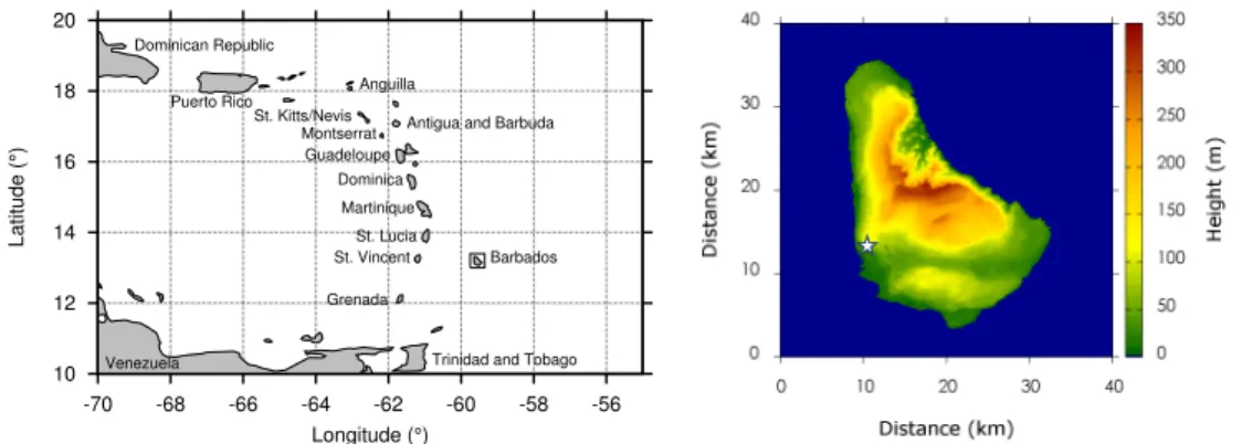
A series of ground-based and airborne remote sensing measurements took place at and around Barbados during the SALTRACE (Saharan Aerosol Long-range Transport and Aerosol-Cloud-Interaction Experiment) 2013 summer campaign. Since Barbados is the easternmost island in the Caribbean and steady easterly trade winds are present,

5

it is not aﬀ_{ected by other surrounding islands. For that reason, Barbados is suitable}

for island eﬀ_{ect studies both from the measurement and the modeling point of view.}

First of all, mineral dust emitted from the Saharan region is transported for more than 4000 km over the Atlantic Ocean with almost no anthropogenic influence. Dust layers arriving at Barbados can be detected with respect to layer height and thickness as

10

well as aerosol composition. Secondly, cloud studies are possible due to persistent trade wind circulation at the Eastern Caribbean. For example, extensive investigations on shallow cumulus cloud properties and their response to diﬀ_{erent ambient cloud}

condensation nuclei (CCN) number concentrations took place during the CARRIBA (Cloud, Aerosol, Radiation and tuRbulence in the trade wInd regime over BArbados)

15

project in 2010/2011 (Siebert et al., 2013). Within CARRIBA, airborne in-situ measure-ments were conducted east of Barbados. The field site of the Max-Planck Institute for Meteorology (MPI-M) Hamburg/Germany with ground-based instruments is located at the east coast as well. The choice of these locations ensures that the island itself has very little to no influence on the measurements and thus marine boundary layer

20

properties can be accurately investigated. During SALTRACE, the TROPOS (Leibniz Institute for Tropospheric Research, Leipzig) and LMU (Ludwig-Maximilians-Universität Munich) field sites were located at the area of the local Caribbean Institute for Mete-orology and Hydrology (CIMH) near the west coast of Barbados (cf. Fig. 1), whereas the DLR (Deutsches Zentrum f. Luft- und Raumfahrt) research aircraft Falcon was

sta-25

(4)

ACPD

15, 22637–22699, 2015

M. Jähn et al.

Title Page

Tables Figures

◭ ◮

Back Close

Full Screen / Esc

Discussion

P

a

per

|

Discussion

P

a

per

|

Discussion

P

a

per

|

Discussion

P

a

per

|

first two properties primarily influence the atmospheric boundary layer (ABL), gravity waves caused by the latter also propagate within the free troposphere.

There are several works regarding the understanding of airflow and thermodynamic quantities around Barbados. A first detailed observational study using pilot balloon measurements was done by DeSouza (1972) and further interpreted by Garstang et al.

5

(1975). DeSouza’s calculated vertical wind velocity fields showed a daytime divergence and nighttime convergence over the island. Mahrer and Pielke (1976) did a series of two- and three-dimensional numerical studies and found that DeSouza’s calculations only hold for a flat island, because he neglected significant eﬀ_{ects of terrain slope in}

his divergence calculations. Heat island eﬀ_{ects on vertical mixing of aerosols at Cape} 10

Verde islands were studied by Engelmann et al. (2011) using aircraft lidar measure-ments and idealized large eddy simulations (LES) with flat island surfaces. They found indications that the diﬀ_{erential heating and the orographic impact control downward}

mixing of African aerosols, which results in a complex vertical layering over the Cape Verde region. Taking the topographical structures into account, Mahrer and Pielke

15

(1976) pointed out some main characteristics, e.g. diurnal changes in the vertical wind velocity fields downwind (i.e. west coast of Barbados) with sinking motions over the center and western part of the island and an upwind cell oﬀ _{the west coast.}

Consid-ering numerical sensitivity studies by Savijärvi and Matthews (2004, SM04 hereafter), the general conclusion was that these forced rising and sinking motions and their

con-20

secutive eﬀ_{ects can only be explained if island orography is included in the numerical}

models. In their 2-D study, SM04 added a 200 m high central mountain to a 20 km wide island and showed that see-breeze circulations are enhanced by upslope winds dur-ing the day. These topographically forced components will dominate if the large-scale mean wind is in the order of magnitude of at least 10 m s−1, which is the case for

Barba-25

dos. Smith et al. (1997) assigned diﬀ_{erent island structures to di}ﬀ_{erent mountain wake}

(5)

ACPD

15, 22637–22699, 2015

M. Jähn et al.

Title Page

Tables Figures

◭ ◮

Back Close

Full Screen / Esc

Discussion

P

a

per

|

Discussion

P

a

per

|

Discussion

P

a

per

|

Discussion

P

a

per

|

hours (cumulus cloud street). Kirshbaum and Fairman (2015) found that surface fluxes control the downwind circulation strength and the trade inversion controls precipita-tion and thus the disrupprecipita-tion of cloud trails. Other influence factors like terrain height, wind speed and their interactions have multiple impacts on flow regimes, turbulence, cloud trail lengths etc. Another study on island eﬀ_{ects with similar topographical heights} 5

compared to Barbados has been done by Minda et al. (2010). They investigated the evolution of the convective boundary layer (CBL) above Okinawa Island, Japan. It was found that for a flat island simulation, the warmed land already induces a distinct roll cloud that is in agreement with the observations. However, the inclusion of island ter-rain leads to a reinforced moisture uplifts, which in turn induce strong convection that

10

can penetrate into the free atmosphere. Idealized numerical studies have been con-ducted by Kirshbaum and Grant (2012) to investigate the impact of mesoscale ascent (with an island height of 500 m) on cumulus convection. A particular important process with regard to the mean horizontal cloud size has been found. The broader the clouds are, the lower is the fractional entrainment rate in these clouds, which in the end leads

15

to an increase in precipitation rates downstream. A key result from another combined theoretical and numerical study by Kirshbaum and Wang (2014) was that nonlinear in-teractions between mechanical and thermal flow over taller mountains were significant and thus lead to a strengthening of the lee-side convergence band.

There are also many studies where the focus lies on the orographic influence of

20

tall islands (e.g. Hawaii Island or Dominica with mountain heights above 1 km) on the leeward flow and precipitation patterns. Esteban and Chen (2008) state that for a strong trade wind flow, the daily rainfall totals at the windward side of the island of Hawaii show a nocturnal maximum due to the convergence of katabatic flow, whereas for weak trades (≤5 m s−1) the rainfall amounts have its maximum in the late afternoon

25

(6)

ACPD

15, 22637–22699, 2015

M. Jähn et al.

Title Page

Tables Figures

◭ ◮

Back Close

Full Screen / Esc

Discussion

P

a

per

|

Discussion

P

a

per

|

Discussion

P

a

per

|

Discussion

P

a

per

|

creates a rainless area. A complementary study with airborne observations and cloud-resolving modeling for the same island was performed by Minder et al. (2013). The comparison showed that the dynamical structures are very well reproduced but it was diﬃ_{cult to reproduce of the observed rainfall by the model. Overall, mesoscale flow}

controls convection and rainfall over Dominica. At lower wind speeds, the circulations

5

seem to be more thermally driven by solar heating.

The main objective of this work is to study local island eﬀ_{ects on the modification}

of the boundary layer structure, microphysical properties and downwind vertical mix-ing of aerosols for selected days durmix-ing the first SALTRACE field campaign. Regard-ing aerosols, especially Saharan dust, it is known from several studies that notable

10

amounts of mineral dust reach Barbados via long-range transport over the North At-lantic, e.g. from first observations at the end of the 1960s (Prospero et al., 1970; Pros-pero and Carlson, 1970) or from back-trajectory calculations by Ellis and Merrill (1995).

Within this work, the following questions are addressed:

– How has the model setup to be chosen to get an as realistic as possible

represen-15

tation of an island-ocean-system in the trade wind regime through the example of Barbados?

– How do turbulent inflow characteristics and grid spacing aﬀ_{ect the simulation}

re-sults?

– Can the daytime convective island boundary layer explain downward mixing of

20

low-altitude Saharan dust layers?

– Are the simulation results comparable with wind lidar measurements over and in the lee of the island?

This paper is structured as follows. Section 2 deals with the general model setup. There, the numerical method, model physics, computational domain, boundary

condi-25

(7)

ACPD

15, 22637–22699, 2015

M. Jähn et al.

Title Page

Tables Figures

◭ ◮

Back Close

Full Screen / Esc

Discussion

P

a

per

|

Discussion

P

a

per

|

Discussion

P

a

per

|

Discussion

P

a

per

|

and applied to our numerical model and particular setup. Results for two case studies in June 2013 and two sensitivity tests are presented and discussed in Sect. 3. In Sect. 4, the simulation results are compared with Doppler wind lidar data. Section 5 provides a summary and concluding remarks.

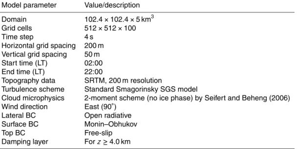
2 Model setup

5

All large eddy simulations are performed with the latest version of the non-hydrostatic, fully compressible All Scale Atmospheric Model (ASAM). An extensive model descrip-tion is presented in Jähn et al. (2015), both covering numerical discretizadescrip-tion methods and physical parameterizations. A special feature of ASAM is the usage of so-called cut cells for the orography. There, a grid box is cut by the intersection of the orographical

10

structure. This method can handle steep terrain gradients and prevents discretization errors compared to traditional methods like terrain-following coordinates, also conserv-ing the original shape of the topography to a high degree.

The following sections give a brief overview of the numerical method and model physics, including governing equations, the subgrid-scale model and the microphysics

15

scheme. After that, the computational domain, boundary conditions (BC), data initial-ization and forcings for the cases of study are described, together with the method to generate inflow turbulence.

2.1 Numerical method and model physics

ASAM numerically solves the fully compressible flux-form Euler equations:

20

∂ρ

∂t +∇ ·(ρv)=0 , (1)

∂(ρv)

(8)

ACPD

15, 22637–22699, 2015

M. Jähn et al.

Title Page

Tables Figures

◭ ◮

Back Close

Full Screen / Esc

Discussion

P

a

per

|

Discussion

P

a

per

|

Discussion

P

a

per

|

Discussion

P

a

per

|

∂(ρφ)

∂t +∇ ·(ρvφ)=−∇ ·qφ+Sφ. (3)

Here,ρis the total air density,v =₍_u_,_v_,_w₎T _{is the three-dimensional velocity vector,}_p

is the air pressure,gis the gravitational acceleration,Ωis the angular velocity vector of the earth,φis a scalar quantity (representing energy and microphysical variables) and

Sφis the sum of its corresponding source terms. The subgrid scale (SGS) terms areτ

5

for momentum andq_φ for a given scalar. The energy equation in the form of Eq. (3) is represented by the density potential temperatureθ_ρ(Emanuel, 1994):

θρ=θ

1+_q_v

_R

v Rd

−1

−qc

. (4)

Hence, the air pressure can be diagnosed via the equation of state:

p=_ρR_d_θ_ρ

_p

p0 κm

, (5)

10

whereθ=_T₍_p₀_/p₎κm _{is the potential temperature,}_q

v=ρv/ρis the mass ratio of water

vapor in the air (specific humidity),qc=ρc/ρis the mass ratio of cloud water in the air, p0is a reference pressure andκm=(qdRd+qvRv)/(qdcpd+qvcpv+[qc+qr]cpl) is the

Poisson constant for the air mixture (dry air, water vapor, cloud water, rain water) with

qd=ρd/ρ.Rd and Rv are the gas constants for dry air and water vapor, respectively.

15

The Coriolis parameterf =₂_ω_sin_ϕ=_3.3_×₁₀−5_s−1_{is calculated from a latitude value}

ofϕ=_13.18◦_{, with}_ω_{being the angular velocity of the earth.}

To parameterize the SGS stress terms in Eqs. (2) and (3), a standard Smagorinsky model is used to represent the influence of the eddies smaller than the grid size into the resolved flow structures. The SGS stress terms areτi j=uiuj−uiuj for momentum

20

andqi j=uiqj−uiqj for potential temperature. The eﬀect of subgrid-scale motion on the resolved large scalesτi j is represented by

(9)

ACPD

15, 22637–22699, 2015

M. Jähn et al.

Title Page

Tables Figures

◭ ◮

Back Close

Full Screen / Esc

Discussion

P

a

per

|

Discussion

P

a

per

|

Discussion

P

a

per

|

Discussion

P

a

per

|

whereSi j=12

∂ui

∂x_j + ∂u_j ∂x_i

is the strain rate tensor and νt the turbulent eddy viscosity.

By taking stratification eﬀ_{ects into account, the eddy viscosity is determined by:}

νt=(Cs∆)2max

0,

|S|2

1−Ri

Pr

1/2

(7)

with

Ri=

g θρ

∂θ_ρ ∂z

|S|2

. (8)

5

where∆ _{is a length scale based on the grid spacing,} _C_s=_{0.2 the Smagorinsky}

co-eﬃ_{cient as estimated by Lilly (1967), and using the Einstein summation notation for}

standardization:

|S|= q

2S_{i j}S_{i j} (9)

Ri is the Richardson number and Pr is the turbulent Prandtl number (Lilly, 1962;

10

Smagorinsky, 1963). By using the cut cell approach, tiny and/or anisotropic cells might occur in the vicinity of topographical strcutures. Thus, the length scale has to be a func-tion of all local grid spacings in orthogonal direcfunc-tion and prescribed correcfunc-tion funcfunc-tions (cf. Scotti et al., 1993; Jähn et al., 2015).

The cloud microphysics parameterization is based on the two-moment scheme

15

Seifert and Beheng (2006) with adjustments applied from Horn (2012) and without ice phase. In this scheme, mass and number density of the hydrometeor classes cloud droplets and rain drops are represented. A total of seven microphysical processes is in-cluded: condensation/evaporation, CCN activation to cloud droplets at supersaturated conditions, autoconversion, self-collection of cloud droplets and rain drops, accretion

(10)

ACPD

15, 22637–22699, 2015

M. Jähn et al.

Title Page

Tables Figures

◭ ◮

Back Close

Full Screen / Esc

Discussion

P

a

per

|

Discussion

P

a

per

|

Discussion

P

a

per

|

Discussion

P

a

per

|

and evaporation of rain. The aerosol activation process is prescribed by a power law function based on grid space supersaturations:

NCCN(S)=NCCN,1 %sκ (10)

with the hygroscopicity parameter κ=_{0.462. By having CCN number concentration}

measurements available for diﬀ_{erent supersaturations, an extrapolated value of the} 5

CCN number concentration at 1 % supersaturation can be determined. It is assumed that at a critical supersaturation value ofs_max=_{1.1 % all CCN are activated.}

2.2 Domain and boundary conditions

To simulate atmospheric flow for the island–ocean system, the size of the model do-main has to have appropriate values dependent on the island size. The do-main criterion

10

in this case is that a marine boundary layer has to develop at least several kilometers before it interferes with the island area. Also, the downwind area should approximately be twice of the island width so that resulting structures induced by the island can be properly represented. Since Barbados is a 24 km wide (west–east) and 34 km long (south–north) island, a model domain with a spatial extent of 102.4 km×102.4 km is

15

chosen. The island is located at the domain center. The model top is set to 5 km alti-tude.

Due to the presence of the island area, non-cyclic lateral boundary conditions have to be used. Within the finite volumes/diﬀ_{erences discretization strategy adopted herein,}

a “zero-gradient” boundary condition is applied to all scalars and velocity components

20

at each lateral boundary (north, east, south, west). This means that the boundary-perpendicular flux for these quantities is set to zero, which leads to a simple radiation condition near the outlets with minimal wave reflection. A pressure correction for sound waves is applied to each actual normal velocity component and not to the initial wind profile, which also suppresses artificial wave reflection near the inflow boundary. This

25

(11)

ACPD

15, 22637–22699, 2015

M. Jähn et al.

Title Page

Tables Figures

◭ ◮

Back Close

Full Screen / Esc

Discussion

P

a

per

|

Discussion

P

a

per

|

Discussion

P

a

per

|

Discussion

P

a

per

|

For the top boundary, a free-slip condition is applied, i.e. the gradient of the tangential velocity component is zero. In order to prevent gravity wave reflection, an additional relaxation term is applied on the right-hand-side of the momentum equations:

Φn+1=_{. . .}₋∆_t_·_ρK₍_d₎₍Φn₍_d₎₋Φ0_{) ,} ₍₁₁₎

with a damping function depending on the distance to the top boundaryd:

5

K(d)= (

dfsin2

π

2

d_w−d dw

d < dw,

0 d≥d_w. (12)

This damping layer is applied aboved_w=_{4 km model height (20 vertical layers) with}

a damping parameterdf =1×10−

3

.

Surface boundary conditions are represented by a momentum flux parameterization based on the Monin–Obhukov similarity theory (Monin and Obukhov, 1954):

10

τ_zx=₋_ρC_m_|v_h|u, (13)

τ_zy=₋_ρC_m_|v_h|v. (14)

Cmis the drag coeﬃcient for momentum, which is defined as follows:

Cm= k2

Ψ2

M

, (15)

with

15

Ψ_M=_ln

_z₊_z

0 z0

−φm

_z

L

, (16)

andφmrepresenting the integrated similarity function.Lstands for the Obukhov length

(12)

ACPD

15, 22637–22699, 2015

M. Jähn et al.

Title Page

Tables Figures

◭ ◮

Back Close

Full Screen / Esc

Discussion

P

a

per

|

Discussion

P

a

per

|

Discussion

P

a

per

|

Discussion

P

a

per

|

The topographic data is obtained from the Consortium for Spatial Information (CGIAR-CSI) Shuttle Radar Topography Mission (SRTM) dataset (http://srtm.csi.cgiar. org) at 200 m resolution. A simple smoothing algorithm is applied to guarantee a proper grid pre-processing. In the smoothed data set, the maximum elevation is lowered by about 15 m compared to the raw topography data, which is an acceptable level.

5

Table 1 summarizes the model configuration for the Barbados large eddy simulations performed in Sect. 3.

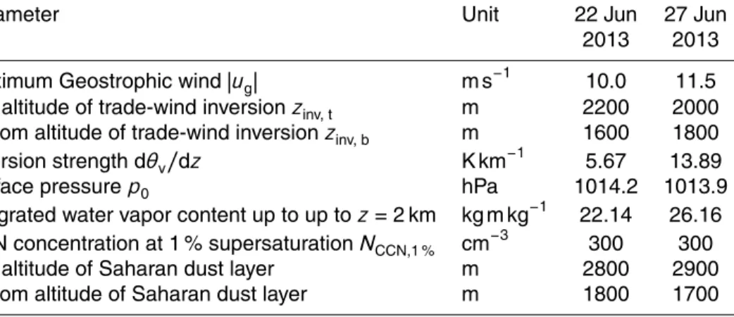
2.3 Initial data

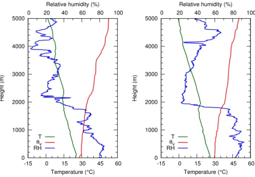
The two cases examined (22 and 27 June 2013) mainly diﬀ_{er in their atmospheric state}

and geostrophic forcing. Measured nighttime radiosonde profiles of temperature and

10

humidity are directly used for model initialization (Fig. 2), which reduces the complexity of the simulations due to the absence of horizontal inhomogeneities and a time-varying background state. There are two reasons behind the choice of using single profiles in-stead of averaging multiple profiles. Firstly, a single initial profile is better for comparing the LES results with Doppler wind lidar data (cf. Sect. 4), which are obtained for a few

15

selected cases during SALTRACE. Secondly, trade-wind inversions are only poorly rep-resented when the soundings are averaged over many cases. This becomes apparent when considering the sharply defined inversion at the 27 June case, which is shown later on. Air density and pressure profiles are obtained by vertical integration with re-spect to hydrostatic equilibrium. Some simplifications are assumed for the geostrophic

20

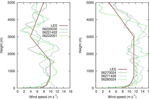
forcing. The wind direction is purely east (i.e. d=₉₀◦ _and _v_g=_{0), which is also for}

simplicity and to make it easier to define upwind and downwind regimes later on. The vertical wind profiles are expressed as piecewise linear functions for both cases, re-spectively. For the 22 June case, the geostrophic wind at first linearly decreases above

(13)

ACPD

15, 22637–22699, 2015

M. Jähn et al.

Title Page

Tables Figures

◭ ◮

Back Close

Full Screen / Esc

Discussion

P

a

per

|

Discussion

P

a

per

|

Discussion

P

a

per

|

Discussion

P

a

per

|

u_g,1=           

−10.0 m s−1 log(z/z0)

log(700 m/z₀), z≤0.7 km

−10.0 m s−1, z≤1.6 km

−10.0 m s−1+_4.29_×₁₀−3_s−1_·₍_z₋_{3000 m) ,} _{1.6 km}_{< z}_≤_{3.0 km}

−4.0 m s−1−2.0×10−3s−1·(z−5000 m) , 3.0 km< z≤5.0 km

(17)

with a roughness lengthz0=0.01 m. A turn in wind direction to southwest is observed

within the layer where the wind speed decreases. However, this is not captured by the LES due to the simplifications and assumptions mentioned above. Therefore, the eﬀ_{ect of wind directional shear might be underestimated in the model for this case.} 5

The change in wind direction (±15◦) is rather small at other altitudes so that the LES input profile can be considered as a good approximation. For the 27 June case, the geostrophic wind linearly decreases abovez=_{3000 m altitude:}

ug,2=       

−11.5 m s−1 log(z/z0)

log(700 m/z₀), z≤0.7 km

−11.5 m s−1, z≤3 km −11.5 m s−1+_5.25_×₁₀−3_s−1_·₍_z₋_{3000 m) ,} _{z >}_{3 km}

(18)

In this profile there is no distinct change in wind direction. Figure 3 visualizes the

10

measured (green lines) and parameterized (red lines) velocity profiles for both cases. The LES background wind profiles are parameterized to closely match the soundings. Within the boundary layer, the LES profile should be near the nighttime measurements (dark green line) because this is mainly a representation of the marine boundary layer. For the free troposphere, the LES profile should roughly be a mean of all three

sound-15

ings, since no large-scale advection term is applied on the wind components during the simulation time.

Table 2 shows a comparison of the two simulated cases with respect to mean flow properties, trade inversion strength, moisture load (all derived from radiosonde pro-files), CCN concentrations (obtained by ground-based measurements at Ragged Point

(14)

ACPD

15, 22637–22699, 2015

M. Jähn et al.

Title Page

Tables Figures

◭ ◮

Back Close

Full Screen / Esc

Discussion

P

a

per

|

Discussion

P

a

per

|

Discussion

P

a

per

|

Discussion

P

a

per

|

station) and the location of the Saharan dust layer (estimated from BERTHA lidar mea-surements at CIMH). The diﬀ_{erences in the geostrophic forcing are already discussed.}

Regarding the atmospheric stability, there is a much stronger trade inversion for the 27 June case with a local virtual potential temperature gradient of 14 K km−1. As men-tioned in the introduction, the trade inversion controls the amount of precipitation and

5

the lifetime of cloud streets. Furthermore, there is a 18 % stronger moisture load for the 27 June case, where a faster cloud development is expected. Due to the vertical and temporal variability of the CCN number concentrations, a mean value of 300 cm−3 has been chosen for both cases, which is a typical magnitude for days with a moderate dust load, where aerosol optical depths between 0.2 and 0.4 are observed.

10

2.4 Forcings

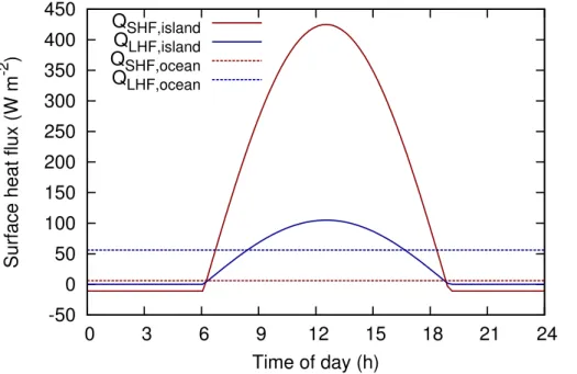
Surface sensible and latent heat fluxes over the island and the ocean are obtained by separate 1-D simulations with full model physics. The parameterizations there in-clude the radiation scheme (Fu and Liou, 1993) as well as land-use and soil mod-els. The soil class “loam” was chosen to represent the average island soil type.

Hy-15

draulic and thermal parameters of this soil type can be found in Doms et al. (2011) and Jähn et al. (2015). For land surface parameterization, “shrubland” appears to be a good compromise between coastal beach areas and forest in the island interior. The roughness length of this land type iszR,island=0.2 m, whereas the ocean roughness

length is set tozR,ocean=0.01 m. The usage of direct (compared to interactive) fluxes

20

reduces computational costs for the LES runs and makes it easier to potentially repro-duce these simulations by other models, especially due to a large number of existing radiation and land-use models. Figure 4 shows the diurnal variation of sensible and latent heat fluxes over the island area. The maximum sensible heat flux over the is-land isQSHF_max,island= 425 W m−

2

and the corresponding maximum latent heat flux is

25

QLHF_max,island= 105 W m− 2

. Surface heat fluxes over the ocean are constant during the whole simulation time withQSHF,ocean=6 W m

−2

andQLHF,ocean=56 W m −2

(15)

ACPD

15, 22637–22699, 2015

M. Jähn et al.

Title Page

Tables Figures

◭ ◮

Back Close

Full Screen / Esc

Discussion

P

a

per

|

Discussion

P

a

per

|

Discussion

P

a

per

|

Discussion

P

a

per

|

at 05:36 LT and sunset is at 18:29 LT, whereby the fluxes are shifted by 30 min to repre-sent the delay due the fact that the soil has to be heated first before energy exchange with the lower atmosphere can take place.

Later on, reference simulations with periodic boundary conditions are performed to obtain information of marine boundary layer characteristics. For these simulations,

5

large-scale forcings from the BOMEX LES study of trade wind cumulus convection (Siebesma et al., 2003) are applied. They include a piecewise linear subsidence veloc-ity profile with an absolute peak value of−560 m day−1, radiative cooling of−2 K day−1 and large-scale advection of dry air into the lower boundary layer of−1 g kg−1day−1:

wsub=     

−4.33×10−6s−1z, z≤1500 m

−0.0065+_1.08_×₁₀−5_s−1_·₍_z₋_{1500 m) ,} _{1500 m}_{< z}_≤_{2100 m}

0.0 , z >2100 m

, (19)

10

dθ

dt =           

−2.315×10−5K s−1, z≤1500 m −2.315×10−5K s−1+_2.315_×₁₀−8_{K s}−1_m−1

·(z−1500 m) , 1500 m< z≤2500 m

0.0 , z >2500 m

, (20)

dq_v

dt =     

−1.2×10−8s−1, z≤300 m

−1.2×10−8s−1+₆_×₁₀−11_s−1_m−1_·₍_z₋_{300 m) ,} _{300 m}_{< z}_≤_{500 m}

0.0 , z >500 m

(21)

2.5 Turbulence generation – the cell perturbation method

LES modeling technique has the advantage of allowing explicit resolution of turbulent production and part of the inertial range scales, being today the most accurate and

15

(16)

ACPD

15, 22637–22699, 2015

M. Jähn et al.

Title Page

Tables Figures

◭ ◮

Back Close

Full Screen / Esc

Discussion

P

a

per

|

Discussion

P

a

per

|

Discussion

P

a

per

|

Discussion

P

a

per

|

domain into the area of interest. In order to ensure that the incoming boundary layer characteristics at Barbados correspond to fully-developed turbulence consistent with the imposed marine boundary layer forcing, we use the cell perturbation method re-cently proposed by Muñoz-Esparza et al. (2014). The cell perturbation method uses a novel stochastic approach based upon finite amplitude perturbations of the potential

5

temperature field applied within a region near the inflow boundaries of the LES domain. This method has demonstrated superior performance when compared to a state-of-the-art synthetic turbulence generator and is computationally inexpensive (Muñoz-Esparza et al., 2015).

Previous studies where the cell perturbation method was developed and validated

10

dealt with transitions from smooth mesoscale flow to nested LES (Muñoz-Esparza et al., 2014, 2015). In these idealized cases, boundary conditions at the LES domain boundaries were imposed from the mesoscale model instantaneous solution (Dirich-let boundary conditions), in which moisture eﬀ_{ects were not considered. Herein, we}

further extend the application of the cell perturbation method to turbulence inflow

gen-15

eration for cloud modeling including terrain eﬀ_{ects. As explained in earlier sections,}

zero-gradient open radiative lateral boundary conditions need to be used in order to minimize wave reflections at the boundaries that do develop in fully-compressible codes like ASAM-LES model when the domain includes terrain features. In order to test the best configuration for the cell perturbation method in this particular context, we

per-20

form a series of calculations where only the upstream region of the Barbados island is considered (i.e. incoming marine boundary layer). The reduced subset of the domain consists of a 51.2 km×51.2 km area in the horizontal, with the same vertical extent and large-scale forcing described in Sect. 2.4 for the 22 June 2013 case study. To represent the marine boundary layer conditions that are going to be imposed through the entire

25

simulation period, constant sensible and latent heat fluxes ofQSHF,ocean=6 W m −2

and

QLHF,ocean=56 W m −2

are used (see Fig. 4).

(17)

ACPD

15, 22637–22699, 2015

M. Jähn et al.

Title Page

Tables Figures

◭ ◮

Back Close

Full Screen / Esc

Discussion

P

a

per

|

Discussion

P

a

per

|

Discussion

P

a

per

|

Discussion

P

a

per

|

is the maximum potential temperature perturbation, and the perturbations are random and uniformly distributed in the intervalh−θepm,+θepm

i

. Three square cells adjacent to the east boundary are used, which were found to provide the fastest transition to a fully-developed turbulent state (Muñoz-Esparza et al., 2015). The cell size is set to 4×4 grid points, to ensure the cell wavelength falls within the inertial range of three-dimensional

5

turbulence. The perturbation time scale, tp, was obtained from Γ =tpU1(4dx) −1₌

1 (Muñoz-Esparza et al., 2015) withU1 being the horizontal wind speed in the first

ver-tical layer, resulting in a frequency to seed instantaneous perturbations oftp=145 s.

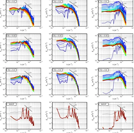
Figure 5 shows instantaneous contours of vertical velocity atz=_z_i_/₂=_{375 m for di}ﬀ

er-ent perturbation Eckert numbers,Ec=_{0.2, 0.33, 0.4 and for the non-perturbation case} 10

(NOCP,Ec=_∞_{). The cell perturbation method for the three}Ecnumbers considerably accelerates the formation of three-dimensional turbulent structures that agree with the ones obtained in the reference simulation using periodic lateral boundary conditions (not shown). As the perturbation Eckert number increases (maximum perturbation am-plitude decreases), the strength of the vertical velocities induced by the temperature

15

perturbations is progressively reduced, and the onset of forcing-consistent turbulence seems to qualitatively occur at earlier distances from the inflow boundary. In contrast, the NOCP case exhibits the formation of coherent streamwise bands, with homoge-neous amplitude and spacing across the entire streamwise extension of the domain. This pattern diﬀ_{ers from the observed features in the convective boundary layer case} 20

analyzed by Muñoz-Esparza et al. (2014), where buoyancy-induced turbulence de-veloped progressively as the flow was advected away from the inflow boundary. We attribute this eﬀ_{ect to the use of zero gradient lateral boundary conditions, where there}

is no “clean” flow imposed at the boundaries and the convection from the imposed heat flux at the surface does not have a predominant location to initiate and rather develops

25

everywhere in the domain and at the same rate.

(18)

ACPD

15, 22637–22699, 2015

M. Jähn et al.

Title Page

Tables Figures

◭ ◮

Back Close

Full Screen / Esc

Discussion

P

a

per

|

Discussion

P

a

per

|

Discussion

P

a

per

|

Discussion

P

a

per

|

development of the upper-wavenumber portion of the energy spectrum for theuandv

components. The larger scales (lower wavenumbers) require longer distances to be es-tablished due to large buoyant plumes having to emerge from the surface and populate across the entire extent of the boundary layer. This flow development pattern is con-sistent with the findings from Muñoz-Esparza et al. (2014) for convective conditions. In

5

contrast, the energy spectrum for the vertical velocity reveals a rapid growth of turbulent energy that reaches levels 10 times greater than the periodic quasi-equilibrium solution (dashed black line), and that progressively dissipate as the flow transitions through the domain. We attribute this behavior to the cell size, 4dx, which for the resolution em-ployed in this study may fall in the vicinity of the limit of the inertial range. Smaller cell

10

sizes were not considered due to the energy dissipation at high wavenumbers present in finite diﬀ_{erences/volumes discretizations. There, an interaction with fully-resolved}

scales and an instigation of an accelerated transition to a developed turbulence state would not have taken place. In addition, the use of zero-gradient lateral boundary con-ditions helps to maintain the signature of the perturbations more than in the case of

15

Dirichlet boundary conditions, hence contributing to strengthen the periodically seeded perturbations. By increasing the perturbation Eckert number from 0.2 to 0.4 (first row vs. third row in Fig. 6), the energy overestimation is damped, and results after a fetch of 40 km forEc=_{0.4 are in close agreement with the periodic simulation used as}

ref-erence and have reached quasi-equilibrium converged statistics. The Ec=_{0.2 case} 20

results in energy deficit at wavenumbers close to the integral length scale, and also at the highest wavenumbers for thew component. When the cell perturbation method is not used (NOCP panels, bottom row in Fig. 6), dramatic energy deficits are found, together with an unrealistic spiky energy distribution in which the expected energy pro-duction and cascade processes are not present.

25

Finally, we examine the vertical distribution of relevant boundary layer quantities at a downstream distance of 40 km from the east boundary (i.e., x=_{11.2 km). Vertical}

profiles (Fig. 7) show the best agreement with the periodic simulation for theEc=_0.4

(19)

ACPD

15, 22637–22699, 2015

M. Jähn et al.

Title Page

Tables Figures

◭ ◮

Back Close

Full Screen / Esc

Discussion

P

a

per

|

Discussion

P

a

per

|

Discussion

P

a

per

|

Discussion

P

a

per

|

structure. Momentum flux profiles exhibit slightly larger values in the first 250 m, due to the diﬀ_{erences in the horizontal wind speed distribution near the surface. However,}

the boundary layer structure is similar, with the diﬀ_{erences being related to distinct}

quasi-equilibrium solutions for the periodic and the open boundary condition simula-tions. Similar conclusions are found for the sensible and latent heat fluxes. The cell

5

perturbation method was originally developed and tested in the context of dry bound-ary layers (Muñoz-Esparza et al., 2014, 2015). It is worth emphasizing that we have herein demonstrated for the first time, as it can be seen from the latent beast flux profile, that the cell perturbation method has the ability to develop turbulent moisture features that are in agreement with the imposed forcing. The Ec=_{0.2 case fails to produce} 10

a boundary layer structure that is similar to the reference periodic case, with exces-sive mixing attributed to an enhanced eﬀ_{ect of the perturbations for the reasons before}

mentioned. Also, the NOCP case does not provide realistic turbulent boundary layer features corresponding to a strongly under-developed turbulent state. Therefore, we select theEc=_{0.4 setup as the inflow to be used for the island simulations presented} 15

in the remaining of the manuscript since it produces the most rapid development and stabilization of forcing-consistent turbulence. For the island cases, we use a domain with horizontal extent of 102.4 km×102.4 km, which leaves suﬃ_{cient fetch for the}

ma-rine boundary layer to develop prior to start interacting with the topography of Barbados and its local stability eﬀ_ects.

20

3 Results

To investigate the eﬀ_{ects of the Barbados island area on boundary layer properties,}

cloud generation and vertical mixing of aerosols, we define two subdomains that are considered to be representative for the upwind and downwind area, respectively. Fig-ure 8 shows the position of these two subdomains. They both cover a base area of

25

(20)

bound-ACPD

15, 22637–22699, 2015

M. Jähn et al.

Title Page

Tables Figures

◭ ◮

Back Close

Full Screen / Esc

Discussion

P

a

per

|

Discussion

P

a

per

|

Discussion

P

a

per

|

Discussion

P

a

per

|

ary layer) is approximately 15 km away from the eastern boundary to avoid contami-nation from the inflow boundaries where turbulence has to be generated first. Looking into the model data, it becomes apparent that at least half of the island area has to be overflown until a well-mixed convective layer can fully develop. For that reason, the downwind subdomain is located between 35 km< x <45 km and thus covers the west

5

coast island area and the marine oﬀ_{shore area in equal parts. The following analysis}

mainly consists of comparisons between these two regimes to investigate island eﬀ_ects

on various parameters.

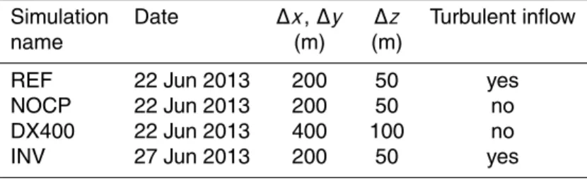
3.1 Overview of performed simulations

Besides the two mentioned case studies, two additional sensitivity studies are part

10

of the island eﬀ_{ect analysis. Here, the 22 June 2013 case serves as reference case}

(REF). For the first sensitivity case (NOCP), the cell perturbation method is disabled so that the upwind flow is strongly underdeveloped. With this setup, the eﬀ_{ect of}

hav-ing a realistic turbulent boundary layer around the island rather than idealized constant winds is investigated. In the next sensitivity case (DX400), the grid resolution is halved

15

from 200 to 400 m horizontally and from 50 to 100 m vertically to point out the deficien-cies in the use of coarser resolution without appropriate resolved turbulence and gray zone modeling (Wyngaard, 2004) for particular aspects of interest in boundary layers and cloud modeling. In this simulation, the cell perturbation method is also put oﬀ_since

the usage of a turbulent inflow in coarse resolution studies has not been utilized before

20

and, moreover, appears to be questionable because the inertial subrange of the turbu-lence spectrum is not resolved anymore. The simulation ensemble is completed by the 27 June 2013 case, mainly characterized by its strong trade-wind inversion (INV) and stronger background trade winds compared to the REF case. Table 3 summarizes the settings for all simulations that deviate from the standard configuration in Tables 1 and

25

(21)

ACPD

15, 22637–22699, 2015

M. Jähn et al.

Title Page

Tables Figures

◭ ◮

Back Close

Full Screen / Esc

Discussion

P

a

per

|

Discussion

P

a

per

|

Discussion

P

a

per

|

Discussion

P

a

per

|

3.2 Boundary layer and cloud characteristics

To get a qualitative impression of the local situation simulated by the LES model, Fig. 9 shows a three-dimensional snapshot of the temperature and humidity field as well as cumulus clouds with up- and downdrafts visualized by isosurface fields at 12:00 LT for the reference case. The daytime convection is clearly visible by multiple updraft cells

5

distributed over the whole island area, which subsequently leads to the development of non-precipitating shallow cumulus clouds. Advection of heated air from the central and southern part of the island towards the west can be seen in the surface temperature field (which is meant as temperature of the lowest model layer in this context), whereas the cooler marine flow narrows the thermal wake toward the meridional center of the

10

domain up to 40 km downwind. This eﬀ_{ect is connected with an island-induced change}

of wind speed and direction. The change of the humidity profile can be observed in the vertical cut plane at the western model boundary. A large amount of moisture is transported vertically upwards in the central region where also occasional cumulus clouds are present. A few ten kilometers away in they direction, dryer air from heights

15

of 500–1000 m is mixed downward.

For further insight into flow dynamics, especially for the downwind region, Fig. 10 provides the vertical wind field at z≈z_i/2 for all four considered cases. Looking at the REF and INV case, several turbulent updraft bands with lengths of about 10 km in zonal direction and vertical velocities up to 2.5 m s−1develop all over the island area.

20

However, one main band aty≈52 km remains persistent, even at higher altitudes. This updraft band is a result of the dynamic and thermal instability over the island, forming quasi two-dimensional horizontal vortex rolls with their axes aligned in the downwind direction (e.g. Etling and Brown, 1993). Toward the evening, as the surface sensible heat flux is not positive anymore and convection fades away, the band decouples from

25

(22)

ACPD

15, 22637–22699, 2015

M. Jähn et al.

Title Page

Tables Figures

◭ ◮

Back Close

Full Screen / Esc

Discussion

P

a

per

|

Discussion

P

a

per

|

Discussion

P

a

per

|

Discussion

P

a

per

|

case, these updrafts are a bit weaker, which is most likely due to the stronger mean horizontal wind speed. Wave-like structures in the upwind vertical velocity field are observed in the NOCP case. There, the flow remains laminar in this region and since no perturbation is applied but surface fluxes are present, these artificial convergence lines are forming. Note that this eﬀ_{ect is not seen in the REF and INV case. This} 5

underscores the importance of having an explicit inflow turbulence generation when working on LES scales. Just by visibly comparing the “coarse” simulation DX400 with the other cases, it becomes apparent that there is a lot of structure loss in the vertical wind field. All up- and downdraft bands – even the main updraft band downwind – are almost perfectly aligned inx direction. This shows the importance of using a grid

10

spacing that resolves the inertial subrange of the velocity spectrum (cf. Bryan et al., 2003). Note that with coarser grid spacings the orographical structures of the island are also less represented.

Figure 11 shows the surface wind fields and liquid water path for all simulated cases at 14:00 LT. In all these cases, the island convection aﬀ_{ects both the strength (up to} 15

4 m s−1stronger wind speeds compared to marine surface winds) and direction (±30◦) of the wind in the downwind area of Barbados, thus leading to strong surface con-vergence and subsequently forming the updraft band as seen in Fig. 10 aty =_{52 km.}

Despite having this elongated band, very little cloud formation is observed in this area for the REF, NOCP and INV cases, which is also the case for other times of the day (not

20

shown). This means that no continuous cloud street is modeled on the 22 June 2013 and the 27 June 2013, respectively. While cloud streets occur on around 60 % of undis-turbed days, there are several eﬀ_{ects that suppress cloud street generation (Kirshbaum}

and Fairman, 2015). In the REF (and NOCP) case, the relatively low moisture load (RH=_{80 % near the surface, decreasing below 60 % at}_z_≈_{1300 m) and a weak trade} 25

(23)

ACPD

15, 22637–22699, 2015

M. Jähn et al.

Title Page

Tables Figures

◭ ◮

Back Close

Full Screen / Esc

Discussion

P

a

per

|

Discussion

P

a

per

|

Discussion

P

a

per

|

Discussion

P

a

per

|

are horizontally aligned to the mean wind direction in the NOCP case. In the REF and INV cases, more realistic scattered cumulus cloud fields over the island area and downwind are modeled. Besides the distinct cloud bands, the DX400 case shows fur-ther very notable diﬀ_{erences in the cloud field. First of all, clouds are broader because}

of the coarser grid spacing. In addition to that, a continuous cloud street is modeled,

5

which can be considered as an artifact since such a cloud band is neither seen in other simulations nor in satellite observations. Furthermore, the downwind horizontal veloc-ity field is slightly stronger compared to the other cases. We attribute this behavior to the lack of resolved small scales that cannot extract energy from the large eddies and therefore grow and become more coherent. This eﬀ_{ect is also observed to a lesser} 10

extent for the NOCP case.

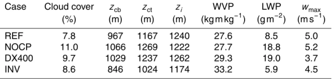
In the following, the diurnal development of the convective island boundary layer is investigated. Figure 12 shows time series of boundary layer and cloud properties for the downwind region around the west coast of Barbados. Further mean quanti-ties of boundary layer and cloud characteristics are diagnosed and summarized in

15

Table 4. The REF and the INV case have some properties in common. They both show a strong increase of cloud cover in the downwind region between 07:00 and 08:00 LT up to a maximum value of about 16 %. The boundary layer heightz_i displays a diur-nal variation, growing up toz=_{1350 m around 13:00 LT in the REF case. For the INV}

simulation,zi is approximately 100–150 m shallower. This parameter is calculated via

20

the Bulk Richardson criterion, where the boundary layer height is defined as the height where the Bulk Richardson numberRi_bexceeds a value of 0.25, with

Ri_b= g

θv0

θ_v−θ_v0

u2₊_v2z, (22)

where θv0 is the virtual potential temperature at the surface. Being relatively similar

in boundary layer characteristics and cloud cover, there is a clear distinction between

25

(24)

ACPD

15, 22637–22699, 2015

M. Jähn et al.

Title Page

Tables Figures

◭ ◮

Back Close

Full Screen / Esc

Discussion

P

a

per

|

Discussion

P

a

per

|

Discussion

P

a

per

|

Discussion

P

a

per

|

mean LWP values as well as in the cloud base and top heights (cf. Table 4). The cloud cover, however, is fairly comparable for these two cases. Peak updraft values also show a diurnal variation, starting from approximatelywmax=1 m s−

1

(which is equivalent to the upwind area value) up towmax=7 m s

−1

around noon. The DX400 case has overall weaker peak updrafts, however this does not mean that there is less vertical transport

5

of energy, moisture, momentum etc. Due to the coarser grid spacing in every spatial direction there is a higher net upward transport.

To further investigate daytime-dependent vertical mixing and layering, Fig. 13 shows hourly averaged vertical profiles boundary layer and cloud parameters for the down-wind domain compared to the daily updown-wind average. Comparing again the REF and INV

10

cases, daytime dependent diﬀ_{erences in the density potential temperature and specific}

humidity profiles can be noticed (not shown). Lower levels atz <700 m are warmer and dryer compared to the marine background. The vertical turbulent transport is evidenced by the profiles of sensible and latent heat fluxes. The sensible heat flux is linearly de-creasing within the mixing layer up to heights between 700 m< z <900 m, depending

15

on the time of day. The maximum latent heat fluxes occur between 600 m< z <800 m. Above that layer, the cloud water content reaches its maximum, which is connected to latent heat release and thus to an increase of the sensible heat flux and a decrease of the latent heat flux. In the INV case, the trade inversion aroundz≈2000 m inhibits further cloud development above this height, whereas in the REF simulation there is

20

also a notable amount of cloud water above 2000 m. The presence of wind shear above 1500 m height leads to a secondary maximum of TKE aroundz=_{2000 m, which is not}

the case in the shearless INV simulation.

In the NOCP case, i.e. without a turbulent inflow, persistent updraft bands form over the island area, which is consistent with the modeled cloud field from Fig. 11. The

25

inflow characteristics have little eﬀ_{ect on boundary layer properties like TKE, vertical}

(25)

ACPD

15, 22637–22699, 2015

M. Jähn et al.

Title Page

Tables Figures

◭ ◮

Back Close

Full Screen / Esc

Discussion

P

a

per

|

Discussion

P

a

per

|

Discussion

P

a

per

|

Discussion

P

a

per

|

already vertically transported some amount of energy, which is missing in the NOCP case. More remarkable diﬀ_{erences are noticeable with regard to cloud development.}

The LWC aroundz≈1000 m during noon is nearly doubled for the NOCP case. There is also a particularly pronounced secondary maximum of LWC aroundz≈2100 m in the same order of magnitude. Taking the average over the whole daytime period, the

5

mean LWP is more than doubled in the NOCP case compared to the REF case, which is in agreement with higher LWC values and also higher cloud cover (≈+_{3 %).}

More undesired eﬀ_{ects become apparent when using a coarser spatial resolution as}

in the DX400 case, which is most noticeable in the averaged vertical profiles. First of all, there is less variability in the potential temperature and specific humidity fields for

10

altitudesz >1000 m, which can be explained by the lack of turbulent vertical transport within the boundary layer (this eﬀ_{ect can be seen in the vertical profile of TKE in Fig. 13}

and in the profile of the vertical velocity variance). The LWC however has maximum val-ues of 0.028 g m−3 aroundz≈2000 m, which is factor 2 higher compared to the REF case. This is accompanied by strong latent heat fluxes in these layers. Cloud growth is

15

also more inhibited at finer resolutions due to explicit entrainment of dryer environmen-tal air (e.g. Bryan et al., 2003). Having a distinct and quite symmetric diurnal variation of boundary layer and cloud properties in the other cases, the evening transition in the DX400 case is poorly represented, where still a notable amount of clouds exist and a deeper boundary layer is modeled around 20:00 LT.

20

3.3 Vertical mixing of aerosols

After the long-range transport of Saharan dust into the Caribbean region, these dust layers arrive at Barbados having mean base heights of about 1.5–2 km a.s.l. Due to a possible interaction with the convective island boundary layer, vertical mixing of aerosols is investigated in this subsection. As already shows in Sect. 2, these aerosol

25

(26)

ACPD

15, 22637–22699, 2015

M. Jähn et al.

Title Page

Tables Figures

◭ ◮

Back Close

Full Screen / Esc

Discussion

P

a

per

|

Discussion

P

a

per

|

Discussion

P

a

per

|

Discussion

P

a

per

|

(2011). These relative concentrations can be related to mass concentrations of Saha-ran dust, e.g. 180 µg m−3. This mass concentration and the Saharan dust layer heights are estimated from ground-based multi-wavelength aerosol lidar measurements (Moritz Haarig, personal communication, 20 July 2015) and provide a rough idea of the mag-nitude of these quantities. Figure 14 displays height-distance profiles of the boundary

5

layer tracerφBLT and the Saharan dust tracerφSDTnear the west coast of Barbados.

In both cases, the turbulent character over the island section is visible as a vertical distribution of the passive tracer within the higher boundary layer and the correspond-ing decrease in tracer concentration. It is and more pronounced for the southern part of the island, which is due to the broader land area width (20 km in the south

com-10

pared to 10 km in the north). It also indicates the wind shear at the island boundaries (e.g. aty=_{43 km), which causes the advection of air masses from}_{z >}_{700 m into the}

boundary layer. This eﬀ_{ect is more pronounced further west (not shown). In the REF}

case, the mean boundary layer height around noon was calculated to bezi ≈1400 m. The passive tracer analysis additionally shows some local overshoots up to over 2 km

15

height asl. These convective instabilities are also seen in the isentropic field (black lines in Fig. 14). The Saharan dust tracers do have a diﬀ_{erent vertical structure. For}

the REF simulation, the tracer is thinned out, with maximum concentrations between 1.9 km< z <2.4 km, whereas in the INV case it is between 1.7 km< z <2.5 km. There are also no overshoots visible beyondz=_{1.7 km. The stronger turbulent mixing in the} 20

REF case can be explained by the presence of wind shear aroundz≈1.5 km height, whereas in the INV case the strong trade wind inversion suppresses further develop-ment of turbulence in higher altitudes.

Although there are already some indications of downward aerosol transport, a bet-ter quantification of these eﬀ_{ects is still needed to achieve a better understanding of} 25