Characterization of a boreal convective boundary layer and its impact on atmospheric chemistry during HUMPPA-COPEC-2010

(1)

ACPD

12, 13619–13665, 2012

Characterization of a boreal convective

boundary layer

H. G. Ouwersloot et al.

Title Page

Abstract Introduction

Conclusions References

Tables Figures

◭ ◮

Back Close

Full Screen / Esc

Printer-friendly Version Interactive Discussion

Discussion

P

a

per

|

Dis

cussion

P

a

per

|

Discussion

P

a

per

|

Discussio

n

P

a

per

Atmos. Chem. Phys. Discuss., 12, 13619–13665, 2012 www.atmos-chem-phys-discuss.net/12/13619/2012/ doi:10.5194/acpd-12-13619-2012

Atmospheric Chemistry and Physics Discussions

This discussion paper is/has been under review for the journal Atmospheric Chemistry and Physics (ACP). Please refer to the corresponding final paper in ACP if available.

Characterization of a boreal convective

boundary layer and its impact on

atmospheric chemistry during

HUMPPA-COPEC-2010

H. G. Ouwersloot1,2, J. Vil `a-Guerau de Arellano1, A. C. N ¨olscher2, M. C. Krol1, L. N. Ganzeveld3, C. Breitenberger2, I. Mammarella4, J. Williams2, and

J. Lelieveld2

1

Meteorology and Air Quality, Wageningen University, Wageningen, The Netherlands

2

Max Planck Institute for Chemistry, Mainz, Germany

3

Earth System Sciences – Climate Change, Wageningen University, Wageningen, The Netherlands

4

Department of Physics, 00014 University of Helsinki, Finland

Received: 13 April 2012 – Accepted: 22 May 2012 – Published: 1 June 2012

Correspondence to: H. G. Ouwersloot (huug.ouwersloot@wur.nl)

(2)

ACPD

12, 13619–13665, 2012

boundary layer

Title Page

Tables Figures

◭ ◮

Back Close

Full Screen / Esc

Discussion

P

a

per

|

Dis

cussion

P

a

per

|

Discussion

P

a

per

|

Discussio

n

P

a

per

|

Abstract

We studied the atmospheric boundary layer (ABL) dynamics and the impact on at-mospheric chemistry during the HUMPPA-COPEC-2010 campaign. We used vertical profiles of potential temperature and specific moisture, obtained from 132 radio sound-ings, to determine the main boundary layer characteristics during the campaign. We

5

propose a classification according to several main ABL prototypes. Further, we per-formed a case study of a single day characterized as a convective boundary layer to analyse the influence of the dynamics on the chemical evolution of the ABL, using a systematic analysis that can easily be extended to other periods during HUMPPA-COPEC-2010. We used a mixed layer model, initialized and constrained by

observa-10

tions. In particular, we investigated the role of large scale atmospheric dynamics (sub-sidence and advection) on the ABL development and the evolution of chemical species concentrations. We find that, if the large scale forcings are taken into account, the ABL dynamics are represented satisfactorily. Subsequently, we studied the impact of mix-ing with a residual layer aloft durmix-ing the mornmix-ing transition on atmospheric chemistry.

15

The time evolution of NOxand O3concentrations, including morning peaks, can be ex-plained and accurately simulated by incorporating the transition of the ABL dynamics from night to day. We demonstrate the importance of the ABL height evolution for the representation of atmospheric chemistry. Our findings underscore the need to couple the dynamics and chemistry at di_fferent spatial scales (from turbulence to mesoscale)

20

in chemistry-transport models and in the interpretation of observational data.

1 Introduction

The boreal forest, located roughly between 50◦and 65◦N, is an ecosystem type that covers 8 % of the global land surface and 27 % of the forested area, covering about 15×106km2 (Williams et al., 2011). Therefore, its impact on the global atmospheric

25

(3)

ACPD

12, 13619–13665, 2012

boundary layer

Title Page

Tables Figures

◭ ◮

Back Close

Full Screen / Esc

Discussion

P

a

per

|

Dis

cussion

P

a

per

|

Discussion

P

a

per

|

Discussio

n

P

a

per

present in the combined ecosystems on Earth, perturbations in the climate of the Northern Hemisphere could lead to changes in the carbon cycle (including emissions of volatile organic compounds, VOCs) and aerosol formation and consequently alter the atmospheric composition (Sellers et al., 1997). Considering the extent of the bo-real forest, perturbations in this ecosystem may alter the dynamics and chemistry at

5

different temporal and spatial scales, up to the entire globe. Therefore, it is relevant and timely to study the processes in the boreal forest at a range of scales in order to understand how they interact and influence the atmospheric dynamics and chemistry.

During the HUMPPA-COPEC-2010 campaign (Williams et al., 2011), which took place at the Finnish SMEAR II station from 12 July to 12 August 2010, special

em-10

phasis was placed on obtaining a complete data set of surface and atmospheric mea-surements to comprehensively characterize the atmospheric physics and chemistry. Guided and constrained by this data, we focus on the influence of large scale forcings and transitions in the morning from nocturnal to daytime conditions on the boreal atmo-spheric boundary layer (ABL) dynamics and the associated atmoatmo-spheric chemistry. Our

15

research extends on the analyses of previous campaigns, like the Boreal Ecosystem-Atmosphere Study (BOREAS) (Sellers et al., 1997). BOREAS was conducted in the Canadian forest, aimed at improving the understanding of interactions between the boreal forest biome and the lower atmosphere (Sellers et al., 1997). Observations in-cluded dynamical, ecological and biogeochemical variables. The latter inin-cluded

obser-20

vations of the trace gases CO2, CH4and non-methane hydrocarbons. Even though the boundary layer dynamics were analysed (Barr and Betts, 1997; Davis et al., 1997), their evolution was not represented using models to identify and quantify acting processes. In addition, their impact on the atmospheric chemistry was not considered.

At the SMEAR II station in Hyyti ¨al ¨a (61◦51′N, 24◦17′E, 181 m a.s.l.) continuous

ob-25

(4)

obser-ACPD

12, 13619–13665, 2012

boundary layer

Title Page

Tables Figures

◭ ◮

Back Close

Full Screen / Esc

Discussion

P

a

per

|

Dis

cussion

P

a

per

|

Discussion

P

a

per

|

Discussio

n

P

a

per

|

vations are performed in the soil, the canopy and the lower part of the ABL. Previous observational campaigns at this site focused on aerosol studies (Nilsson et al., 2001).

During the HUMPPA-COPEC-2010 campaign the standard instruments of the SMEAR II site were complemented with additional equipment. An overview of the gas and aerosol measurement instruments is given in Table 1 of Williams et al. (2011). To

5

be able to characterize the ABL evolution, additional observations were made to obtain vertical profiles of the meteorological variables, using a Cessna aircraft and radioson-des. The campaign turned out to be of particular interest due to the anomalously high temperatures that might be representative of future boreal climates. Since the atmo-spheric temperature affects the surface latent and sensible heat fluxes (van

Heerwaar-10

den et al., 2010), future climates may be characterized by di_fferent ABL dynamics. Concentrations of chemical species in the atmosphere are governed by surface exchange, chemical processes and dynamics in the ABL. Therefore, it is imperative to correctly represent the ABL dynamics when interpreting or predicting atmospheric chemistry (Davis et al., 1994; Ganzeveld et al., 2008; Vil `a-Guerau de Arellano et al.,

15

2011). A primary goal of our research is to determine how the growth of the ABL in-fluences atmospheric chemistry. The ABL height development inin-fluences the chemical evolution of the boundary layer in two ways. First, the actual height of the ABL can be considered as a mixing volume in which reactive compounds are released. During the day, the height of this layer increases non-linearly from values as low as 100 m in the

20

morning to values that can exceed 2 km in the afternoon. Second, the growth of the boundary layer determines the entrainment of air from the free troposphere into the boundary layer. This entrained air generally has different thermodynamic and chemical properties than air in the ABL.

In this paper we classify different boundary layer prototypes that correspond to the

25

(5)

ACPD

12, 13619–13665, 2012

boundary layer

Title Page

Tables Figures

◭ ◮

Back Close

Full Screen / Esc

Discussion

P

a

per

|

Dis

cussion

P

a

per

|

Discussion

P

a

per

|

Discussio

n

P

a

per

scales, the atmospheric dilution capacity and the entrainment of free tropospheric air. An overview of these processes is given in Table 1 of Ouwersloot et al. (2011).

We further examine the boundary layer dynamics for a single day with particularly intensive observations, using a mixed layer model (MXL). Emphasis is placed on how atmospheric chemistry is a_ffected by the ABL height evolution. The day is selected

be-5

cause important processes took place that can be easily overlooked when analysing the impact of the boundary layer dynamics on chemistry. These processes, associated with temporal transitions and large-scale forcings, include subsidence, the advection of air masses and, in the morning, the connection with a residual boundary layer of the previous day. We complete the study by evaluating the effectiveness of the

ap-10

plied observational strategy during HUMPPA-COPEC-2010 in characterizing the ABL dynamics.

The next section covers the methodology of this study. Subsequently, the represen-tation of the boundary layer height during one representative day in the HUMPPA-COPEC-2010 campaign is presented. This is followed by an illustration of its

impor-15

tance for accurately modelling atmospheric chemistry. Finally, the strategy for obtaining meteorological data during field campaigns is discussed.

2 Methods

In this study, meteorological and atmospheric chemistry observations are combined with numerical experiments. Some observations serve as initial and boundary

con-20

ditions, while others are compared to the numerical model results. The upper atmo-spheric conditions are determined by radiosondes and the atmoatmo-spheric conditions near the Earth’s surface are obtained at the SMEAR II measuring station. The used chem-ical observational techniques are described in Table 1 of Williams et al. (2011). We focus on the O3observations with the ultraviolet absorption/fluorescence (UV) method

25

(6)

ACPD

12, 13619–13665, 2012

boundary layer

Title Page

Tables Figures

◭ ◮

Back Close

Full Screen / Esc

Discussion

P

a

per

|

Dis

cussion

P

a

per

|

Discussion

P

a

per

|

Discussio

n

P

a

per

|

were all performed by the Max Planck Institute for Chemistry at a height of 24 m above the ground.

Two complementary numerical techniques are used: the mixed layer model is applied to characterize the boundary layer dynamics and their possible effect on atmospheric chemistry, while vertical profiles generated in the numerical experiments with a

Large-5

Eddy Simulation (LES) model act as virtual radio soundings for the discussion of the observed radiosonde profiles. More specific information is given in the following sec-tions.

2.1 Radiosondes

During the campaign, 175 GRAW DFM-06 radiosondes have been launched from

10

a clear area at approximately 300 m distance from the main observational site. In prin-ciple, five radiosondes were launched per day at the local daylight saving times (LT, UTC+3) 3:00, 9:00, 12:00, 15:00 and 21:00. The local daylight saving time is ahead of the local solar time by 1 h 29 min. During intensive observation periods (IOP), the frequency of radiosonde launches was increased to intervals of maximum two hours.

15

These events took place from 16 July 21:00 to 17 July 18:00, from 21 July 21:00 to 22 July 18:00, from 28 July 21:00 to 29 July 18:00 and from 5 August 18:00 to 6 August 18:00. The observations of 6 August will be analysed in more detail.

Data transmitted by the sonde each second was received by an antenna placed at a nearby building. Next to a GPS device, each sonde included a temperature and

20

a humidity sensor. The GPS coordinates were used to determine the altitude and geo-graphical location of the sonde, as well as the wind velocities. The determined position is accurate within 10 m and the uncertainty of the wind velocity measurements is less than 0.1 m s−1. The temperature sensor measured with an accuracy of 0.2◦C and the humidity sensor measured the relative humidity with an accuracy of 1 %. The software

25

(7)

ACPD

12, 13619–13665, 2012

boundary layer

Title Page

Tables Figures

◭ ◮

Back Close

Full Screen / Esc

Discussion

P

a

per

|

Dis

cussion

P

a

per

|

Discussion

P

a

per

|

Discussio

n

P

a

per

relative humidity data, the profiles of the potential temperature,θ, and specific humidity,

q, are determined. This study focuses on the lowest 3000 m of these profiles.

2.2 SMEAR II data

Data near the surface was gathered at the boreal forest observational station SMEAR II (Hari and Kulmala, 2005). The standard observations include meteorological data,

5

aerosols and the concentrations of several chemical species (CO2, H2O, CO, O3, SO2, NO and NO2). In addition, the turbulent fluxes of temperature, moisture, momentum, aerosols, CO2, O3 and several volatile organic compounds are measured. For this study, the heat fluxes, surface pressure, relative humidity and temperature observations are used.

10

The sensible heat flux,H, and the latent heat flux, LE, are determined using 30-min averages over 10 Hz Eddy Covariance measurements at a height of 23 m (Mammarella et al., 2009). The observations were made above the canopy top, which was located at approximately 15 m height. As such they can be considered as appropriate surface forcings for the development of the ABL and can be directly related to the ABL dynamics

15

observed from the radiosonde profiles.

The observational data of surface pressure and the relative humidity and tempera-ture at 50 m height originate from the SMEAR smartSearch database (Junninen et al., 2009). These data are converted to potential temperature and specific humidity in a similar way as the radiosonde data.

20

2.3 Mixed layer model (MXL)

To represent and subsequently interpret the observational data, a mixed layer model is used that is coupled to a chemical module (Tennekes, 1973; Vil `a-Guerau de Arellano et al., 2009). This model is based on the zeroth-order mixed layer assumption that dur-ing the day turbulent mixdur-ing is vigorous enough to result in a well-mixed ABL. Thus, the

25

(8)

ACPD

12, 13619–13665, 2012

boundary layer

Title Page

Tables Figures

◭ ◮

Back Close

Full Screen / Esc

Discussion

P

a

per

|

Dis

cussion

P

a

per

|

Discussion

P

a

per

|

Discussio

n

P

a

per

|

theory assumes that conserved scalar variables are uniformly distributed in the vertical direction and that their fluxes are therefore characterized by linear profiles. A thermal inversion layer caps the ABL and separates it from the free troposphere. Both the ther-mal inversion layer and the surface layer (lowest 10 % of the boundary layer, Stull, 1988) are considered to be thin compared to the total boundary layer. This approach

5

has first been used by Lilly (1968), Tennekes (1973), Carson (1973) and Betts (1973). The vertical profiles of the evaluated quantities show a discontinuity at the height of the inversion, above which they linearly change with height in the free troposphere accord-ing to their free tropospheric gradients. This simplified representation of the ABL, which nevertheless incorporates the processes under study, allows for numerical experiments

10

in which atmospheric chemistry and basic ABL dynamics are simultaneously solved at very low computational costs. A model that is similar to the one used here, including chemistry, is described by Vinuesa and Vil `a-Guerau de Arellano (2005). Further devel-opment includes expanding the chemical module and taking the influence of specific humidity on the entrainment rate into account (Vil `a-Guerau de Arellano et al., 2009).

15

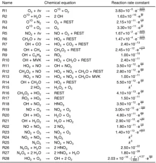
The chemical module is flexible and enables the use of different chemical schemes. In previous work it has mostly been used to represent the O₃-NO_x-VOC-HO_xsystem that is typical for the Amazonian rain forest. The currently applied chemical scheme, which is based on the scheme used by van Stratum et al. (2012), is presented in Table 1. The model acts as a support for the observational data, enabling to study the evolution of

20

the main properties of the boundary layer dynamics.

More information about the governing equations is given in Appendix A.

2.4 LES model (DALES)

To evaluate the use of radio soundings to obtain vertical profiles of temperature and moisture, numerical experiments have been performed with the modified 3.2 version of

25

(9)

ACPD

12, 13619–13665, 2012

boundary layer

Title Page

Tables Figures

◭ ◮

Back Close

Full Screen / Esc

Discussion

P

a

per

|

Dis

cussion

P

a

per

|

Discussion

P

a

per

|

Discussio

n

P

a

per

local observations. In addition, DALES enables us to study how atmospheric flows that are induced by heterogeneous surface forcings influence the distribution of both thermodynamic and chemical variables.

This specific LES model has first been used by Nieuwstadt and Brost (1986) and fur-ther developed and improved since (e.g., Cuijpers and Duynkerke, 1993; Dosio et al.,

5

2003). Processes are explicitly resolved on scales larger than a set filter width and parametrized on the smaller scales at which the eddies contain less energy. The re-solved equations are the filtered Navier-Stokes equations upon which the Boussinesq approximation is applied (Heus et al., 2010). Typically, the filter width is chosen such that over 90 % of the turbulent energy is contained in the resolved scales. The

subfilter-10

scale parametrization is based on the one-and-a-half-order closure assumption (Dear-dorff, 1973). Periodic boundary conditions are applied in the horizontal directions.

The version of DALES used for this study is modified to enable studies of ABL flows characterized by heterogeneous boundary conditions at the surface (Ouwersloot et al., 2011) and to generate local instantaneous vertical profiles of the chemical species

15

mixing ratios and the dynamical variables. This allows for a comparison between ra-diosonde profiles and the profiles that are predicted by numerical experiments

3 Results

3.1 Boundary layer prototypes

Our interpretation of the radiosonde observations indicates that during

HUMPPA-20

COPEC-2010 no clear trend due to synoptic influences is present and that the charac-teristics of the ABL significantly differ each day. Therefore, the boundary layer dynamics and their influence on atmospheric chemistry have to be analysed on a day-to-day ba-sis. To support this analysis, it is convenient to have a first classification of the ABL dy-namics during HUMPPA-COPEC-2010 and associate the radiosonde measurements

25

(10)

ACPD

12, 13619–13665, 2012

boundary layer

Title Page

Tables Figures

◭ ◮

Back Close

Full Screen / Esc

Discussion

P

a

per

|

Dis

cussion

P

a

per

|

Discussion

P

a

per

|

Discussio

n

P

a

per

|

thus be linked to the representations in combined chemistry-meteorology models. The prototypes are characterized by specific vertical profiles and the associated dynami-cal processes (e.g., Stull, 1988). During the campaign, three different prototypes were observed that correspond to the most representative vertical potential temperature pro-files. Out of the 175 radiosondes 43 could not be classified by these prototypes, either

5

due to instrumental errors or different (transitional) characteristics in the observed verti-cal profiles. We select three profiles from the radiosonde observations to describe their main characteristics. The profiles are presented in Fig. 1.

Figure 1a shows the potential temperature profile observed at 16:00 LT on 17 July. It is characterized by a relatively constant potential temperature with height, topped by

10

a layer of a few hundred meters in which the vertical gradient of the potential tempera-ture gradually increases. The location of the maximum potential temperatempera-ture gradient marks the height of the boundary layer (Sullivan et al., 1998), in this case at approxi-mately 2150 m. From the top of the ABL, the potential temperature linearly increases with height, following the free tropospheric gradient. This increasing potential

temper-15

ature profile indicates a region that is characterized by a stably stratified flow. The potential temperature is approximately equal in the entire boundary layer due to con-vective mixing. The jump in potential temperature at the top of the boundary layer, i.e. the thermal inversion, acts as a cap and limits the exchange of air between the ABL and the free troposphere. This measured profile is associated with the convective

20

boundary layer that is usually formed by active convective turbulence during the day. As mentioned in Sect. 2.3, a commonly used approximation, the zeroth-order jump as-sumption (Garratt, 1992), assumes the inversion layer as infinitesimally small, resulting in a jump in the potential temperature at the top of the boundary layer. The resulting theoretical profile is plotted with dashed lines. This very common boundary layer

proto-25

(11)

ACPD

12, 13619–13665, 2012

boundary layer

Title Page

Tables Figures

◭ ◮

Back Close

Full Screen / Esc

Discussion

P

a

per

|

Dis

cussion

P

a

per

|

Discussion

P

a

per

|

Discussio

n

P

a

per

temperature is again constant. However, in this case this mixed layer is topped with a conditionally unstable layer. This type of ABL is normally observed with active shallow cumulus (fair weather) clouds (Stull, 1988). The conditionally unstable layer is located between the mixed layer and the inversion layer and is characterized by an increase with height of the potential temperature that is stronger than the dry and weaker than

5

the moist adiabatic lapse rate. The dry adiabatic lapse rate is defined as the increase of potential temperature that an unsaturated rising air parcel would experience under adiabatic conditions, while the moist adiabatic lapse rate describes this increase for a saturated rising air parcel. In short, the conditionally unstable layer acts as a turbu-lence suppressing stable layer for unsaturated air parcels and as a turbuturbu-lence

gener-10

ating unstable layer for saturated air parcels. In the first case (clear air), this layer can be considered as part of the thermal inversion layer, while in the latter case (clouds) air parcels that enter the layer rise to its top. When this profile was observed, the hu-midity was too low to result in condensation (below 70 % relative huhu-midity) and clouds. If under such conditions condensation would have occurred for local air parcels in the

15

conditionally unstable layer, the resulting clouds would become active and grow. Above the conditionally unstable layer, the thermal inversion is located at a height of 2500 m. Above the inversion, the potential temperature rises according to the free tropospheric profile. The corresponding boundary layer prototype, shown by the black dashed line, is a mixed layer topped with a conditionally unstable layer.

20

The third radiosonde profile is depicted in Fig. 1c and is based on data obtained at 3:00 LT on 7 August. It shows a potential temperature that increases with height in a layer that reaches up to a few hundred meters above the surface. Aloft the potential temperature is relatively constant with height. On top, a thermal inversion at 1700 m and a free tropospheric profile are present. This data is characteristic for nocturnal

25

(12)

ACPD

12, 13619–13665, 2012

boundary layer

Title Page

Tables Figures

◭ ◮

Back Close

Full Screen / Esc

Discussion

P

a

per

|

Dis

cussion

P

a

per

|

Discussion

P

a

per

|

Discussio

n

P

a

per

|

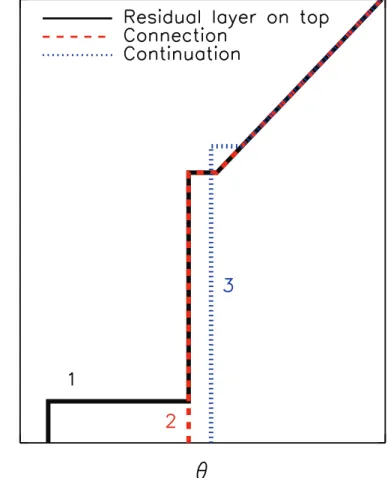
be present above the stable boundary layer, as is the case in this example. However, this is not the case for all stable boundary layers and residual layers can disappear as time progresses (Kaimal et al., 1976). After sunrise, the Earth’s surface warms and convective turbulence mixes the air. The stable boundary layer characteristics are then dissipated and a new convectively mixed boundary layer is formed. If a residual layer

5

is still present, the new mixed layer develops until the potential temperature is equal in both layers. When this happens, buoyant thermals that originate at the surface enter the residual layer without passing through a stable atmospheric layer, a process called overshooting. It results in an almost instantaneous mixing of the new boundary layer with the air masses in the residual layer. From that moment on, mixed layer theory can

10

be applied to study the evolution of the combined ABL. This process of connecting a shallow boundary layer with a residual layer is depicted in Fig. 2. Its impact will be analysed in more detail in Sect. 3.4, putting special emphasis on the evolution of the concentrations of the chemical species NO₂and O₃.

An overview of the occurrence of all three boundary layer prototypes during

15

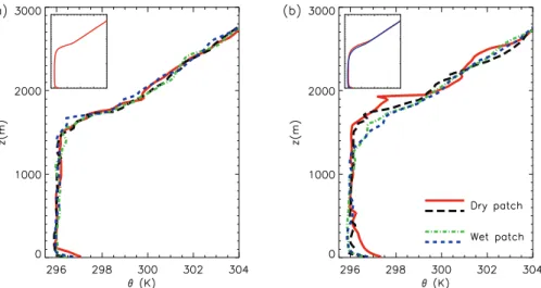
HUMPPA-COPEC-2010 is given in Table 2. Note that the radiosonde profiles in Fig. 1 are selected based on their unambiguous structure. In general, due to the instanta-neous measurements, deviations of the radiosonde profile compared to the domain averaged profile occur, caused by different atmospheric processes. One of these, which is often overlooked, is the influence of land surface heterogeneity on the distribution of

20

temperature, moisture and chemical species. To show that these deviations are realis-tic, Fig. 3 presents local instantaneous potential temperature profiles as generated by DALES. This simulation is based on the period between 12:00 and 15:00 LT of the MXL case that is treated in more detail in Sect. 3.2. The resolution of the domain is 50 m in the horizontal direction and 20 m in the vertical direction. The numerical grid spans

25

(13)

ACPD

12, 13619–13665, 2012

boundary layer

Title Page

Tables Figures

◭ ◮

Back Close

Full Screen / Esc

Discussion

P

a

per

|

Dis

cussion

P

a

per

|

Discussion

P

a

per

|

Discussio

n

P

a

per

a sensible and latent heat flux of 295 W m−2 and 262 W m−2, respectively. In case of heterogeneous surface forcings, the domain is split into two patches in thex-direction, thedry and thewet patch. The kinematic surface heat flux is increased (decreased) by 0.04 K m s−1 and the kinematic surface moisture flux is decreased (increased) by 0.017 g kg−1m s−1for thedry (wet) patch. It appears from Fig. 3a that for the

homoge-5

neous surface forcings, even though the domain averaged profile is smooth (inset), the individual profiles slightly differ from each other and show more random behaviour due to the turbulent character of the ABL, i.e. local warm and cold parcels of air. As demon-strated by the blue dashed line, this can result in observed boundary layer heights that differ from the domain average. Figure 3b shows that the differences between local

in-10

stantaneous profiles are enhanced for heterogeneous surface forcings, especially over the patch with the higher sensible heat flux. This is due to the generated mesoscale circulations (Ouwersloot et al., 2011) in the ABL. These local differences should be kept in mind during the analysis of the radiosonde profiles.

3.2 Diurnal evolution of the ABL 15

To describe the boundary layer dynamics in greater depth, a specific day is selected, characterized by a boundary layer of the mixed layer type. The chosen day, 6 August 2010, was scheduled as an IOP, so multiple radio soundings were performed at rel-atively short time intervals (every 2 h) during the day. The profiles of θ and q show clear mixed layer prototype behaviour (Fig. 1a) for these soundings, which enables the

20

analysis of the data using the MXL model. The day is of interest for the interpretation of chemical observations, since most instruments were functioning and the wind came from the south-west, which was its predominant direction (Table 2 of Williams et al., 2011). Therefore, chemical data is available for this day under conditions that are typ-ical for the campaign. Closely related to our research questions, additional dynamtyp-ical

25

(14)

ACPD

12, 13619–13665, 2012

boundary layer

Title Page

Tables Figures

◭ ◮

Back Close

Full Screen / Esc

Discussion

P

a

per

|

Dis

cussion

P

a

per

|

Discussion

P

a

per

|

Discussio

n

P

a

per

|

processes include advection of air masses, subsidence and the coupling of a dynam-ically evolving boundary layer with a residual layer aloft during the morning transition. The advection and subsidence are both related to forcings on the meso- and synoptic scale. Note that under typical conditions for which subsidence occurs (high pressure and temperature), the emissions of primary biogenic compounds are usually larger

5

(e.g., Guenther et al., 2006; Yassaa et al., 2012).

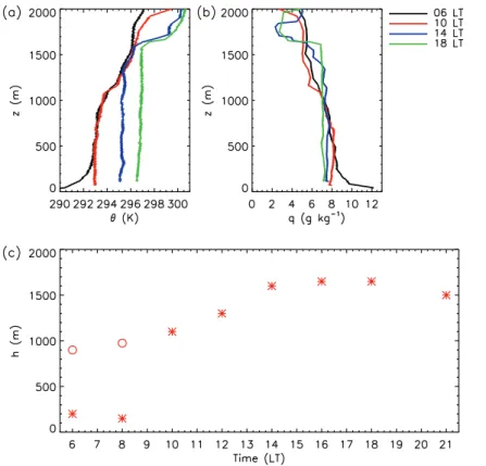
Figure 4 shows the time evolution of the boundary layer dynamics as observed by the radiosondes. The vertical profiles of potential temperature and specific humidity are displayed in Fig. 4a and 4b, respectively. For clarity, only four profiles (at 6:00, 10:00, 14:00 and 18:00 LT) are presented out of the eight available ones (at 6:00, 8:00, 10:00,

10

12:00, 14:00, 16:00, 18:00 and 21:00 LT). We omit the radiosonde profiles near the surface (until 100–300 m) due to the poor reception of the sonde data by the antenna of the ground station if the sonde is at lower heights. At higher altitude, the signal is less perturbed and data is received regularly. In Fig. 4c, the evolution of the boundary layer height is presented. Boundary layer heights are denoted by stars, while the top of

15

the residual layer (in the morning) is denoted by circles.

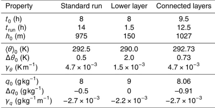
To initialize the MXL model, the vertical profiles of the potential temperature and spe-cific humidity for an initial point in time are applied. For this study, the residual layer in the observations at 8:00 LT is chosen as initial profile. Since the residual layer is much deeper than the underlying shallow mixed layer (975 m and 150 m, respectively) and

20

both layers connect and mix within the first hours of the day (between 8 and 10 LT), considering the residual layer as a start of a new mixed layer seems a valid approxi-mation.

The radiosonde observations are also used to derive the effects of large scale sub-sidence (downward moving air) and advection. These effects can not be observed

di-25

(15)

ACPD

12, 13619–13665, 2012

boundary layer

Title Page

Tables Figures

◭ ◮

Back Close

Full Screen / Esc

Discussion

P

a

per

|

Dis

cussion

P

a

per

|

Discussion

P

a

per

|

Discussio

n

P

a

per

as the difference between these two velocities, as expressed by Eq. (A4). To derive the contribution of the horizontal advection of air masses we take a di_fferent approach. The horizontal advection of air, with different dynamical and/or chemical properties, results in an increase or decrease in the mixed layer averaged scalars. In our model this rate of change is considered to be constant in time. Therefore, a di_fference between the

5

observed and modelled scalar values that increases linearly in time is considered to be caused by advection. For the case under study we find that the advection of cooler air is of importance for temperature (with a cooling rate of 0.108 K h−1 resulting in a max-imum difference of 1.5 K), whereas there is no significant contribution of advection to humidity. This approach cannot be directly applied to the advection of chemical species,

10

since the free tropospheric concentrations are unknown. In addition, di_fferences can be caused by unaccounted chemical pathways.

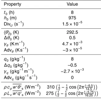
The prescribed sensible and latent heat fluxes in the MXL model are determined by fitting sinusoids through the observed fluxes, as shown in Fig. 5a. The complete set of initial conditions and forcings is presented in Table 3. In Fig. 5 b–d, the

simu-15

lated evolutions of the main dynamical ABL characteristics are shown together with the observations. This shows that the model reproduces the radiosonde observations for temperature, moisture and boundary layer heights well. Until approximately 17:00 LT, entrainment most strongly influences the ABL height development, resulting in a deep-ening ABL. When the boundary layer reaches its maximum height of 1740 m, the

sub-20

sidence velocity for that height is equal in magnitude as the entrainment velocity. By that time the entrainment process is still very active, as the driving heat fluxes are still stronger than 50 % of their maximum values. Since the surface sensible and la-tent heat fluxes continuously decrease after 14:00 LT, the entrainment fluxes weaken as well. Consequently, after 17:00 LT the subsidence becomes stronger than the rate

25

(16)

ACPD

12, 13619–13665, 2012

boundary layer

Title Page

Tables Figures

◭ ◮

Back Close

Full Screen / Esc

Discussion

P

a

per

|

Dis

cussion

P

a

per

|

Discussion

P

a

per

|

Discussio

n

P

a

per

|

convective boundary layer type (Fig. 1a) is not longer applicable. A stable boundary layer appears with a residual layer aloft (Fig. 1c). During the whole day, the advection of relatively cool air results in a decrease of the potential temperature. After 18:00 LT this effect is stronger than the heating effect due to surface fluxes and entrainment, ex-plaining the temperature decline. As shown by the time evolution in Fig. 5d, the specific

5

humidity remains approximately constant, since the effects of the surface moisture flux and the entrainment of relatively dry air cancel each other (∂_∂thqi ≈0).

To determine the importance of advection and subsidence, four different cases have been simulated. The three cases other than the previously derived standard MXL case differ by having the subsidence and/or advection disabled. We omit the effect of

subsi-10

dence by setting DivU=0 s−1and the horizontal advection of air with a different

temper-ature by setting Adv_θ=0 K s−1(Appendix A). First we discuss the impact of subsidence. From Fig. 6a we find that subsidence is significant for the boundary layer height devel-opment on 6 August 2010. In the cases without subsidence the boundary layer grows like a standard convectively mixed boundary layer until approximately 20 LT.

Subse-15

quently, the surface heat flux does not remain positive and the growth stops. Since this layer is no longer actively mixed, it remains as a residual layer on top of the stable nocturnal boundary layer. When subsidence occurs, the boundary layer growth slows down, resulting in lower ABL heights. As mentioned earlier, after 18:00 LT the boundary layer height decreases as the subsidence is stronger than the ABL height increase due

20

to entrainment and the ABL becomes shallower. The rate at which the boundary layer height decreases reaches its maximum when entrainment ceases. The subsidence does not influence the incoming heat fluxes, but does result in shallower boundary layers. Therefore, subsidence promotes a warmer ABL. This is discernible in Fig. 6b.

Figure 6a shows that the advection of relatively cold air from other regions does not

25

(17)

ACPD

12, 13619–13665, 2012

boundary layer

Title Page

Tables Figures

◭ ◮

Back Close

Full Screen / Esc

Discussion

P

a

per

|

Dis

cussion

P

a

per

|

Discussion

P

a

per

|

Discussio

n

P

a

per

as depicted in Fig. 6b. During the day, the impacts of advection and subsidence on the potential temperature roughly cancel in the case under study. Therefore, if both effects are ignored, the resulting potential temperature evolution is similar to that when both effects are concurrently considered. Our results indicate that the effects of both subsidence and horizontal advection are important to take into account.

5

3.3 Importance of the ABL height representation for atmospheric chemistry

After determining the evolution of the ABL dynamics, we study how it influences the mixing ratios of reactive species. Here we focus on the importance of a correct rep-resentation of the boundary layer height. Note that we solely study the primary e_ffect of the boundary layer height evolution on the mixing ratio of chemical species, i.e. the

10

ratio between surface exchange and mixing height (first term on the r.h.s. of Eq. A1). To prevent biases due to a combination of dilution and entrainment (e.g., Vil `a-Guerau de Arellano et al., 2011), the initial mixing ratios are set equal in the boundary layer and the free troposphere. Two atmospheric chemistry cases are evaluated to show the impacts of the ABL dynamics and surface emissions depending on the region under study. For

15

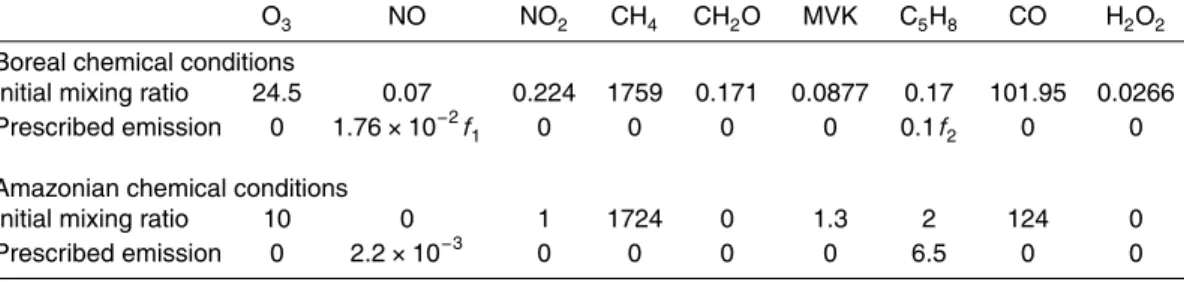
the first case the initial conditions and surface forcings are based on boreal conditions, while a second case is formulated to contrast the boreal forest to the tropical Amazon rainforest conditions. The initial mixing ratios, in ppbv, and the emissions at the surface, in mg m−2h−1, are set to 0, except for the values listed in Table 4.

We designed three different numerical experiments: a “realistic” case, a constant 20

case and a case that considers the residual layer part of the free troposphere (by ig-noring the residual layer). The three corresponding boundary layer height evolutions are shown in Fig. 7a. The first case corresponds with that described in the previous section, though expanded with the chemistry calculations. Thus the boundary layer height evolution is equal to the one presented above, which represents the

observa-25

(18)

ACPD

12, 13619–13665, 2012

boundary layer

Title Page

Tables Figures

◭ ◮

Back Close

Full Screen / Esc

Discussion

P

a

per

|

Dis

cussion

P

a

per

|

Discussion

P

a

per

|

Discussio

n

P

a

per

|

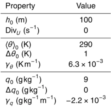
free troposphere aloft is ignored. Therefore, this layer is considered to be part of the free troposphere only and the prescribed initial mixed layer conditions and the free tro-pospheric gradients both change. The effect of subsidence is not considered for this situation. The altered settings for this case are listed in Table 5.

In Fig. 7b the resulting evolutions of the hydroxyl radical (OH) mixing ratio are

pre-5

sented for the boreal conditions. Since the emissions of isoprene (C5H8) are relatively low, and its background concentration is negligible, the depletion of OH is governed by other chemical species (especially CO). As we prescribe uniform initial profiles in the ABL and the free troposphere and neglect surface exchanges for these other chemical species, the resulting time evolutions of OH are very similar. As presented in Fig. 7c,

10

it becomes di_fferent for our case with Amazonian conditions. In this case, the initial concentration and the emission of isoprene are higher and the depletion of OH due to isoprene is significant. During the first six hours of simulated time, if the emitted iso-prene is distributed over a smaller mixing volume, the isoiso-prene concentrations become higher and, consequently, the depletion of OH is enhanced. The constant boundary

15

layer height case, which has the larger mixing volume, therefore starts with the highest OH concentration. The ABL height and OH mixing ratio are lowest for the case that ignores the residual layer. Due to the additionally produced secondary reactants (e.g. through RO2) this effect remains even after the boundary layers reach the same height for two cases. Because of this non-linear effect, the OH mixing ratio remains

high-20

est in the case with the constant boundary layer height and lowest in the case where the influence of the residual layer is ignored. Our findings show that for an adequate model representation of atmospheric chemistry in the boundary layer, it is important to represent the boundary layer height evolution throughout the day. This holds espe-cially for cases in which emitted chemical compounds significantly affect the chemical

25

(19)

ACPD

12, 13619–13665, 2012

boundary layer

Title Page

Tables Figures

◭ ◮

Back Close

Full Screen / Esc

Discussion

P

a

per

|

Dis

cussion

P

a

per

|

Discussion

P

a

per

|

Discussio

n

P

a

per

3.4 Representation of the morning transition

As discussed in Sect. 3.1, in the early morning a residual mixed layer of the previous day is frequently observed above the stable boundary layer and the shallow boundary layer that follows when convection starts. Due to the initially weak surface heat fluxes, the potential temperature in the shallow boundary layer increases until it is similar to the

5

residual mixed layer (in our case around 9:30 LT). Then both layers merge and become one mixed boundary layer, as illustrated in Fig. 2. In the MXL model this merging of two atmospheric layers into one is instantaneous. However, in reality it can take some time due to inhomogeneous ABL conditions and the time it takes for thermals to rise from the surface to the top of the residual layer. In this section we will show that this process can

10

explain specific patterns in the chemistry observations during the morning transition. Note that these numerical experiments do not aim for a perfect representation of the boreal atmospheric chemistry, though demonstrate that this merger of two atmospheric layers is an important process that may explain certain features in the observations of chemical species in the morning.

15

Three numerical experiments were designed. The first, the standard case, corre-sponds to that previously defined in Sect. 3.2, except for the chemical conditions. This case assumes the residual layer to be part of the mixed layer. The second experiment, thelower layer, is based on the initial shallow boundary layer. This corresponds to sit-uation (1) in Fig. 2. The initial values for potential temperature, specific humidity and

20

ABL height are again obtained from the radiosonde observation of 8:00 LT. This numer-ical experiment is run for 1.5 h. After that the buoyant thermals that originate from the shallow boundary layer enter the residual layer and the two layers mix almost instanta-neously, resulting in situation (2) in Fig. 2. The third numerical experiment represents the ensuing combined mixed layer. This case is referred to asconnected layers and

25

(20)

ACPD

12, 13619–13665, 2012

boundary layer

Title Page

Tables Figures

◭ ◮

Back Close

Full Screen / Esc

Discussion

P

a

per

|

Dis

cussion

P

a

per

|

Discussion

P

a

per

|

Discussio

n

P

a

per

|

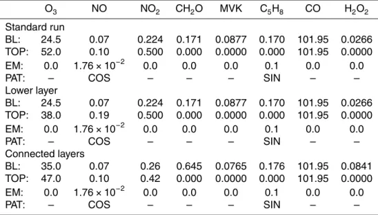
emissions and initial mixing ratios, presented in Table 7 if non-zero, are chosen such that the observations of the isoprene, NO, NO₂and O₃mixing ratios are reproduced.

The observed and modelled mixing ratios of NO2and O3are presented in Fig. 8a and 8b, respectively. The time evolution of NO (not shown) has similar features as that of NO₂. The observations show that in the early morning (until 9:30 LT) the NO₂ mixing

5

ratio rises quickly. This is due to the emission of NOx into the shallow boundary layer. Subsequently, the two atmospheric layers merge. Since the air in the residual layer has lower mixing ratios of NO and NO₂, the mixing ratios in the combined mixed layer are lower than the mixing ratios in the previous shallow boundary layer. Because in reality the conditions of the ABL are not completely horizontally homogeneous, this

10

mixing does not occur simultaneously everywhere, resulting in a transition that takes approximately one hour. After the mixing of the two layers, the NOx contributions of emission and entrainment are still positive, but are distributed over a larger mixing vol-ume. Therefore, their impact becomes weaker and, due to chemical destruction by OH, the NO2 mixing ratio slightly decreases with time. The morning peak in NO2 can not

15

be reproduced by the MXL model if only one numerical experiment is performed. How-ever, by combining two numerical experiments, one for the shallow boundary layer and one for the final combined mixed layer, this peak can be reproduced and explained. It is worthwhile to note that the longer the separation between shallow boundary layer and residual layer remains present, the stronger this morning peak is. Additionally,

20

due to storage in the canopy under a stable boundary layer, NOx could accumulate near the surface during the night. When turbulence sets in, the canopy and ABL air masses interact, which could cause pulses in the surface exchange in the early morn-ing (Ganzeveld et al., 2002).

The O3mixing ratio in Fig. 8b does not show a sudden decrease or increase.

How-25

(21)

ACPD

12, 13619–13665, 2012

boundary layer

Title Page

Tables Figures

◭ ◮

Back Close

Full Screen / Esc

Discussion

P

a

per

|

Dis

cussion

P

a

per

|

Discussion

P

a

per

|

Discussio

n

P

a

per

ratio to rise in the growing shallow boundary layer. During the transition both layers are combined into one mixed layer. The rate of change of O₃in this merged boundary layer is altered due to two reasons: the mixing ratio in the atmospheric layer above the original residual layer is different and the entrained air is mixed over a larger mixing volume after the combination. In effect this results in a slower increase of the O₃mixing

5

ratio. Note that the assumption of one well-mixed boundary layer from the start enables us to get a reasonable first approximation of the mixing ratio evolution. However, the representation in the morning is off and the differences in the rate of change of O₃ before and after 9:30 LT can not be explained. By using the first order approximation to consider in succession thelower layer andconnected layerscases, the time evolution

10

of O₃can be explained and reproduced.

Our findings show that by using a relatively basic modelling tool, the mixed layer model, and using a first order approximation for the combining of a shallow bound-ary layer with a residual layer aloft, important features in the morning observations of chemical species can be reproduced and explained. We therefore conclude that the

in-15

terpretation of atmospheric chemistry observations using a numerical model requires that dynamical processes are accounted for, including the boundary layer height evo-lution and the connection to a residual layer. This supports previous budget studies using the MXL model (Vil `a-Guerau de Arellano et al., 2011; van Stratum et al., 2012) and a single column model (e.g., Ganzeveld et al., 2008).

20

4 Reflection on the observational strategy during HUMPPA-COPEC-2010

In this section, we extend the previous analysis to formulate recommendations for the observational strategy during campaigns such as HUMPPA-COPEC-2010. The experi-ences during the HUMPPA-COPEC-2010 campaign enable us to improve the strategy for future campaigns, resulting in an even more complete and comprehensive set of

25

(22)

ACPD

12, 13619–13665, 2012

boundary layer

Title Page

Tables Figures

◭ ◮

Back Close

Full Screen / Esc

Discussion

P

a

per

|

Dis

cussion

P

a

per

|

Discussion

P

a

per

|

Discussio

n

P

a

per

|

As presented in Fig. 3, local observations can result in variations of the measured scalars under the influence of the boundary layer dynamics. For the potential tempera-ture, the largest variations occur in the surface layer and near the inversion layer. The variability of the scalars is even enhanced by heterogeneous surface forcings (Ouw-ersloot et al., 2011). Thus, we conclude that for representative observations of the

5

boundary layer dynamics it would be recommendable to launch multiple radiosondes simultaneously at key moments (e.g., morning transition, noon and evening transition) to account for the influences of heterogeneous terrain and local, instantaneous obser-vations. In addition, these multiple radiosondes would provide important information about the spatial variations in the dynamical variables, which could be used to evaluate

10

results of numerical models, including large scale chemistry-transport models.

Furthermore, the lowest few hundred meters of the atmosphere are important to characterize in detail. Within a convective boundary layer a surface layer is present in which the profiles of potential temperature, specific humidity and concentrations of chemical species can have significant vertical gradients. The nocturnal boundary layer,

15

characterized by stable stratification, has a similar height as well. However, the obser-vations during HUMPPA-COPEC-2010 did not suffice to fully characterize this part of the ABL. The observations at the towers are only performed at six fixed locations below 67 m and the radiosonde profiles near the surface are occasionally omitted due to poor transmission of the sonde data. To enable the characterization of the nocturnal

bound-20

ary layer and the surface layer during the day, it is recommended to operate kytoons (tethered balloons) (Stull, 1988) with the relevant instruments for at least these lower areas. Due to the tether, no data will be lost and the speed of the ascend/descend during the profiling can be controlled.

As discussed in Sect. 3.2, another possible improvement to the employed

observa-25

(23)

ACPD

12, 13619–13665, 2012

boundary layer

Title Page

Tables Figures

◭ ◮

Back Close

Full Screen / Esc

Discussion

P

a

per

|

Dis

cussion

P

a

per

|

Discussion

P

a

per

|

Discussio

n

P

a

per

(maximum 1 h). After calculating the entrainment velocity from the observed inversion layer properties and surface heat fluxes (Eq. A5), it can be subtracted from the ob-served ABL growth rate to determine the subsidence velocity (Eq. A4). In combination with the horizontal wind direction and velocity, the advection can be calculated from the horizontal gradients of the di_fferent scalars (Eq. A1). The influence of horizontal

5

advection for potential temperature and specific humidity can therefore be determined by simultaneously launching at least 3 radiosondes around the observational site to obtain the horizontal distribution of these scalars. This approach has previously been applied to tower observations (e.g., Aubinet et al., 2003).

As presented in Fig. 4c, the observations during HUMPPA-COPEC-2010 enable

10

a characterization of the development of ABL dynamics. However, for most days ob-servations were limited to 5 radiosonde launches. During the intensive observation periods additional measurements were performed at relatively short time intervals, but even then continuous measurements are not available. A continuous representation of the ABL height would be relevant input for chemical box models as discussed in

15

Sect. 3.3 and demonstrated in Fig. 7. Continuous observations could be obtained using a ceilometer, sodar (Nilsson et al., 2001) or a lidar (Gibert et al., 2007). This would also enable that the morning transition can be studied in greater detail, and more specifically the mixing of a shallow boundary layer with a residual layer aloft. Another advantage of continuous observations would be that fluctuations in the measurements due to local

20

observations can be filtered by time averaging the data, according to Taylor’s frozen turbulence hypothesis (Stull, 1988).

5 Conclusions

By combining observations, both near the surface and in the free troposphere, with a mixed layer model, we studied the atmospheric boundary layer dynamics as

ob-25

(24)

ACPD

12, 13619–13665, 2012

boundary layer

Title Page

Tables Figures

◭ ◮

Back Close

Full Screen / Esc

Discussion

P

a

per

|

Dis

cussion

P

a

per

|

Discussion

P

a

per

|

Discussio

n

P

a

per

|

on the boreal atmospheric chemistry. We investigated the influence of large scale forc-ings (subsidence and advection) and the transition from nocturnal to daytime turbulent conditions on the development of the ABL.

The meteorological data has been classified by identifying boundary layer prototypes based on the vertical potential temperature profiles. During the campaign three di_ff

er-5

ent types were observed: the stable boundary layer, the convectively mixed boundary layer and the conditionally unstable layer above a mixed layer. Of these three types, the convective boundary layer was observed most often, 78 out of the 132 classified soundings. Illustrated by Large-Eddy Simulation model results, we discuss how instan-taneous observed profiles can deviate from these prototypes.

10

By selecting a single day, characterized by a convective boundary layer, 6 August 2010, we studied in detail the key dynamic contributions that influence atmospheric chemistry. This analysis could be applied to other cases observed during HUMPPA-COPEC-2010. It is shown that by using a relatively basic numerical model, the mixed layer model (MXL), the evolution of the boundary layer dynamics can be reproduced

15

and explained. A residual mixed layer in the early morning and the effects of two dif-ferent large scale forcings, subsidence and horizontal advection, have been shown to be important. During this day, the horizontal advection of cold air results in a decrease of the temperature at the measurement site. Subsidence inhibited the boundary layer growth, causing a lower boundary layer height and consequently, due to a smaller

20

mixing volume and unaltered sensible and latent heat fluxes, higher temperatures. By accounting for both subsidence and cold air advection, the modelled evolution for tem-perature was shown to remain approximately equal, though the resulting atmospheric boundary layer height evolution was significantly reduced.

It is demonstrated that the representation of atmospheric chemistry with a

nu-25

(25)

ACPD

12, 13619–13665, 2012

boundary layer

Title Page

Tables Figures

◭ ◮

Back Close

Full Screen / Esc

Discussion

P

a

per

|

Dis

cussion

P

a

per

|

Discussion

P

a

per

|

Discussio

n

P

a

per

not suffice to accurately predict the concentrations of chemical species at that point in time.

The morning transition from a shallow boundary layer, merging with a residual mixed layer aloft into a combined mixed boundary layer, has been represented by combining two numerical experiments with the mixed layer model. The results show that by using

5

this assumption, we are able to explain and represent an observed morning peak in the NOx concentrations and the increase of O3concentrations with time.

By using the mixed layer model, several processes are identified that require atten-tion during observaatten-tional field campaigns if measured data is to be reproduced. We find that emphasis should be placed on continuous observations of the atmospheric

10

boundary layer height, combined with model analyses. Using this combined informa-tion, the effects of mixing with the residual layer and the entrainment and dilution of chemical species can be evaluated. A continuous representation could be achieved by using radiosondes and a numerical model, although this method assumes a bound-ary layer that is characterized by the convective boundbound-ary layer prototype and requires

15

knowledge of the large scale forcings. Therefore, we suggest the use of a ceilometer, sodar or lidar in future campaigns.

Appendix A

Mixed layer equations

The prognostic equations are solved by the mixed layer model for multiple conserved

20

scalar variables,S. These variables are the potential temperature, θ, specific humid-ity,q, and the mixing ratio’s of chemical species, cspecies. θand q influence the evo-lution of the ABL height. Since the ABL is well mixed during the day, the averages of the variables over the whole boundary layer, hSi, can be used for the evaluation. The difference between the free tropospheric and boundary layer values is symbolized

25

(26)

ACPD

12, 13619–13665, 2012

boundary layer

Title Page

Tables Figures

◭ ◮

Back Close

Full Screen / Esc

Discussion

P

a

per

|

Dis

cussion

P

a

per

|

Discussion

P

a

per

|

Discussio

n

P

a

per

|

(Vil `a-Guerau de Arellano et al., 2009):

∂hSi

∂t = w′_S′

s−w′S′e

h −

U∂hSi

∂x +V ∂hSi

∂y

+R_S, (A1)

∂∆S

∂t =γSwe− ∂hSi

∂t . (A2)

An illustration of the different contributions to the boundary layer height development and to the prognostic equation for the boundary layer averaged scalars is presented in

5

Fig. 9. The different terms are explained in more detail below.

w′_S′

s and w′S′e are the surface and entrainment fluxes, respectively. The height of the mixed layer ish.U and V are the wind velocities in the x and y direction and the total term −U∂_∂xhSi+V ∂_∂yhSi is the advection of S, Adv_S. The advection is positive if it leads to an increase in S. R_S expresses additional sources or sinks for scalar S.

10

In the case of a chemical species,R_S is equal to the chemical production minus the chemical destruction of that species, based on the applied chemical mechanism. The vertical gradient in the free troposphere is expressed byγ_S. The velocity at which free tropospheric air is entrained into the boundary layer is symbolized bywe.

The surface fluxes are prescribed, though for the zeroth-order jump assumption the

15

entrainment flux at the top of the mixed layer is expressed by

w′_S′

e=−we∆S. (A3)

Next to the scalar variables, the boundary layer height evolution is included by applying

∂h

∂t =we+ws. (A4)

20

(27)

ACPD

12, 13619–13665, 2012

boundary layer

Title Page

Tables Figures

◭ ◮

Back Close

Full Screen / Esc

Discussion

P

a

per

|

Dis

cussion

P

a

per

|

Discussion

P

a

per

|

Discussio

n

P

a

per

s−1. Note that this represents a linear profile withws=0 at the surface, as presented in Fig. 9b. The entrainment velocity is diagnosed by solving

we=−

w′_θ′

ve ∆θv

(A5)

together with the closure assumption that w′_θ′

ve=−β w′θ′vs, where usually β=0.2. The virtual potential temperature,θv, that appears in this set of equations, is equal to

5

θv=θ(1+0.61q) , (A6)

which results in

w′_θ′

v= 1+0.61q

w′_θ′₊_0.61_{θ w}′_q′_, _(A7)

∆θv= ∆θ+0.61 hqi∆θ+hθi∆q+ ∆θ∆q

. (A8)

Acknowledgements. H. O. gratefully acknowledges financial support by the Max Planck

10

Society. The modelling part of this study was sponsored by the National Computing Facilities Foundation (NCF project SH-060-11) for the use of supercomputer facilities. I.M. acknowledges support from the Academy of Finland Center of Excellence program (project 1118615). The authors thank the colleagues who assisted in launching the radiosondes.

15

The service charges for this open access publication have been covered by the Max Planck Society.

References

Aubinet, M., Heinesch, B., and Yernaux, M.: Horizontal and vertical CO₂advection in a sloping forest, Bound.-Lay. Meteorol., 108, 397–417, doi:10.1023/A:1024168428135, 2003. 13641

20