Feasible domain of Walker's unsteady wall-layer model for the velocity profile in turbulent flows

Printed version ISSN 0001-3765 / Online version ISSN 1678-2690

www.scielo.br/aabc

http://dx.doi.org/10.1590/0001-3765201420130528

Feasible domain of Walker's unsteady wall-layer model for the velocity profile in turbulent flows

MIKHAIL D. MIKHAILOV1 and ATILA P. SILVA FREIRE2

1_{Divisão Científica, Instituto Nacional de Metrologia, Qualidade e Tecnologia}

(DINAM/DIMCI/INMETRO), 22050-050 Rio de Janeiro, RJ, Brasil

2_{Programa de Engenharia Mecânica (PEM/COPPE/UFRJ), Universidade Federal do Rio de Janeiro,}

Caixa Postal 68503, 21945-970 Rio de Janeiro, RJ, Brasil

Manuscript received on January 13, 2014; accepted for publication on May 5, 2014 ABSTRACT

The present work studies, in detail, the unsteady wall-layer model of Walker et al. (1989, AIAA J., 27, 140 – 149) for the velocity profile in turbulent flows. Two new terms are included in the transcendental non-linear system of equations that is used to determine the three main model parameters. The mathematical and physical feasible domains of the model are determined as a function of the non-dimensional pressure gradient parameter (p+). An explicit parameterization is presented for the average period between bursts

(T+

B), the origin of time (t+0) and the integration constant of the time dependent equation (A0) in terms of p +

.

In the present procedure, all working systems of differential equations are transformed, resulting in a very fast computational procedure that can be used to develop real-time flow simulators.

Key words: law of the wall, turbulent boundary layer, unsteady model, feasible domain, asymptotic theory.

INTRODUCTION

Over the last forty years much effort has been placed on understanding the dynamical processes through which turbulence is created and maintained in boundary layers. The implications are evident. Provided a clear picture of the turbulence structure is developed, the basis for the construction of statistical-structural turbulence models is immediately laid down.

Wall-layer models for the innermost portions of the boundary layer are of particular interest. The extreme thinness of the viscous sublayer naturally demands the use of exceptionally fine meshes in the numerical computation of flows. To overcome this difficulty, an elegant method resides on the specification of local analytical solutions that can then be used to represent the properties of the flow throughout the wall layer. This type of approach was originally described in Patankar and Spalding (1967) and is normally referred to as the wall function method.

Most of the research on wall models is historically related to Reynolds averaged Navier-Stokes (RANS) methods; however, this approach has also appropriately served large eddy simulations (LES) of turbulent flows. Piomelli and Ballaras (2002) have reviewed the applicability of some available methodologies to

LES, discussing their assets and drawbacks. In hybrid RANS/LES approaches – whether zonal or non-zonal approaches – wall functions have also been extensively used (see, e.g., Hsieh et al. (2010)) to specify the lower boundary conditions.

Attempts to incorporate the structure of organized motions into near-wall analytical models persist today, but were given particularly interesting contributions through the works of Bark (1975), Hatziavramidis and Hanratty (1979), Chapman and Kuhn (1986), Walker et al. (1989) and Landahl (1990). These authors followed modeling routes that were completely original at the time they were proposed, but to some extent the works did not receive the attention they probably deserved. Here, we concentrate on the analysis of Walker et al. (1989).

The model of Walker et al. (1989) is set on premises that differ somewhat from all the mentioned above; it strives to develop an analytical solution for the time-dependent velocity profile from asymptotic arguments and similarity solutions of a non-homogeneous diffusion equation. The other models, briefly reviewed below, are treated computationally.

Bark (1975) evaluates the fluctuating velocity field with simplified models for the mean velocity distribution and the intermittent Reynolds stress during bursting periods. The model considers how a turbulent boundary layer responds to excitation caused by bursting motions which occur randomly. The length and time scales are considered larger than those typically associated with the bursting phenomenon. The energy spectra of the fluctuating large-scale motions in the wall layer region are resolved by the model.

Hatziavramidis and Hanratty (1979) discuss the numerical solution of the unsteady Navier-Stokes equations in the viscous wall region with simplications resulting from the "slender body" assumption. Their model evaluates the cross-flow velocity field for a flow that is periodic in time and in the direction transverse to the direction of the mean flow. An eddy time-varying model that incorporates observed wavelengths and bursting frequency of the wall eddies is used to formulate the boundary conditions. The near wall flow is driven by the fluctuating pressures originating from the outer flow.

Three distinct models are presented in Chapman and Kuhn (1986). They embody more complex space- and time-dependent boundary conditions at the outer edge of the viscous boundary layer, so as to reflect, as much as possible, the flow structure observed in experiments. Eight physical modeling guidelines are used to characterize the organized quasi-periodic eddy motion near the wall. A comparison between computed turbulence quantities and experiments is presented. The limiting behavior of turbulence near the wall is discussed in terms of power-law expressions.

In Landahl (1990), local intermittent streaks are considered to act locally and for a very short time, setting up the initial conditions for the evolution of three-dimensional perturbations that are considered linear and inviscid. The prescribed model for the initial nonlinear perturbation results in an eddy that is observed to grow linearly in time. The associated Reynolds shear stress is expressed in terms of the lift-up of fluid elements.

The theory of Walker et al. (1989) was given a first glimpse in Walker and Abbott (1976). In fact, some results had previously appeared in reports difficult to find. However, Figure 1 of Walker and Abbott (1976) is exactly Figure 2 of Walker et al. (1989). Therefore, it is clear that, at least for a zero-pressure gradient flow, a time-dependent solution for the instantaneous longitudinal velocity was available as early as 1976. The model of Walker et al. (1989) is formulated in terms of the dynamics of the time-dependent wall-layer flow. A simplified set of the Navier-Stokes (N.-S.) equations is obtained to describe the unsteady flow in the wall layer during a quiescent period. Following the general description commonly found in literature, the flow dynamics is considered to be dominated by two features: wall layer streaks and the bursting phenomenon.

observed over a large characteristic time, the quiescent period (Kline et al. 1967). To determine the mean velocity profile in the wall layer, a time-average of the leading order instantaneous velocity is performed over the average period between bursts, which is considered to be approximately equal to the duration of the quiescent period.

The present work studies, in great detail, the feasible domain of the model proposed by Walker et al. (1989). The definitions of the instantaneous and mean velocity profiles, as preconceived by Walker et al.

(1989), depend on the determination of four unknowns, the average period between bursts (T+B), the origin

of time (t+

0), a constant of integration of the time dependent equation (A0) and the local pressure gradient

(p+). Once p+ is specified, a set of three non-linear equations must be solved to reveal T+_B, t+0 and A0. These

parameters must be real and satisfy T+

B > t+0. In Walker et al. (1989) no comments are made regarding any

possible limitation on the value of p+. Our attempts to find a feasible domain pmin+ ≤ p+≤ pmax+ from the

expressions shown in Walker et al. (1989) failed.

Here, all expressions introduced in Walker et al. (1989) are verified through the MathematicaTM _(Wolfram

2008) software system. In fact, it was later discovered that two terms are missing in equation (63) of Walker

et al. (1989). The resulting non-linear set of equations for parameters T+B, t+0 and A0 is thus correctly presented

and the feasible domain p+

min ≤ p+≤ pmax+ is determined. To find the numerical solution, the system of non-linear

algebraic equations was transformed onto a system of ordinary differential equations with initial conditions. The system was then solved by NDSolve to generate a solution in terms of interpolation functions.

As it turns out, the model developed by Walker et al. (1989) is mathematically feasible in the

domain p+ ₂ [-0.025, 41.886]. To find this interval, the model was only required to provide real values

for the parameters computed from the governing system of non-linear equations and to satisfy the

condition T+

B > t+0; no further stringency to physical validity was required. However, if the model is required to furnish only positive derivatives at the wall for the instantaneous velocity, the feasible

domain is reduced to p+₂ [-0.025, 0.104996].

The present work derives in detail all similarity solutions for the homogeneous diffusion differential partial equation presented in Walker et al. (1989). In doing so, a new treatment is introduced whereby the pressure term is included as a non-homogeneous contribution. To permit fast computations, interpolation functions were generated from initial and boundary value problems, to represent some complex special functions, including Ξ. The special function Ξ (Walker et al. 1989) and its derivatives are given exact expressions (see

Mikhailov and Silva Freire 2012), based on original identities for the hypergeometric functions 1F1 and pFp.

The analysis of Walker et al. (1989) is specially developed for attached flow. The dominance of the error and logarithmic functions over the solution must clearly prevent its use in regions of separated flows

since solutions of the type y2 and y1/2 cannot occur as predicted by Goldstein (1930, 1948) and Stratford

(1959). This aspect of their analysis is further discussed here.

For the first time, an explicit parameterization is presented for T+B, t+0 and A0 in terms of p+. These

expressions make abundantly clear that p+ and _T+

B cannot be independently specified for computations of

the instantaneous velocity profile. They show that once the near wall flow dynamics is accepted to be driven

by dominating diffusion effects, T+

B is determined uniquely by p+.

MODEL FORMULATION

mean-velocity profiles and higher-order statistics. Early studies (Prandtl (1925), von Karman (1930), Coles (1956)) of the attached turbulent boundary layer have successfully split the boundary layer into two typical regions, a viscous (inner) sublayer where turbulent and laminar stresses are of comparable magnitude and a defect (outer) layer where the turbulent stresses provoke a small perturbation to the inertia dominated external flow solution.

The identification of the pertinent length scale δ+ _{(= v/u}

τ, v = kinematic viscosity, uτ = friction velocity)

for the wall region permitted authors to develop local analysis, that naturally lead to analytical solutions (Prandtl (1925), Millikan (1939)) and the advance of proper dimensional arguments. For example, authors have identified the peak production of turbulent kinetic energy to occur at wall distances of the order of

12δ+ (Laufer (1954), Gad-el-Hak and Bandyopadhyay (1994)).

TIME-MEAN STRUCTURE

The time-mean structure of the flow in Walker et al. (1989) is based on the classical two-layered asymptotic analyses (Yajnik (1970), Bush and Fendell (1972), Mellor (1972)) of large Reynolds number turbulent boundary layer flow. Solutions are then developed in terms of two small parameters,

R‒1 and u*, where R denotes the Reynolds number based on representative external flow scales and

u* = uτ /ue,ue = mainstream velocity.

Because the analysis is restricted to the inner layer, the local variables are scaled with u_τ and v

(kinematic viscosity).

The leading-order governing equation of the mean wall flow is set to be (Walker et al. (1989); see also: Loureiro and Silva Freire (2011), Sychev and Sychev (1987), Cruz and Silva Freire (1998)),

@

+

@¾

@

_@

with U+ _{= u / u}

τ,

¾

p+ ₌ v dpe

ρu3

τ dx (2)

where pe denotes the external flow pressure.

The salient aspect of Eq. (2) is that it becomes undetermined at a point of flow separation, xs, since

u_τ = 0. Also note that, at this point, pressure changes greatly across the boundary layer, implying that pe is

not an appropriate reference parameter at the wall (Stratford (1959), Loureiro and Silva Freire (2009, 2011), Loureiro et al. (2008)).

In the outer limit of the wall region, the mean velocity profile, U+, is required to follow a logarithmic

behavior, implying that the dominant effect in Eq. (1) is the Reynolds stress effect.

In the outer region of the wall layer, U+ must satisfy

U+ = ϰ1 ln y+ + Ci, as y+ → ∞ (3)

TIME-INSTANTANEOUS STRUCTURE

To obtain the governing equations of the unsteady flow in the wall layer during a quiescent period, Walker et al. (1989) introduced the following non-dimensional variables,

u+ = u / u_τ, v+ = v / u_τ, w+ = w / u_τ (4)

and

x

~ = x / Lx, y+ = y uτ / v, z+ = z uτ /v, t+ = tu_τ2 /v (5)

where Lx is a characteristic length in the x-direction associated with the longitudinal extent of the

outer-region structures that drive the wall-layer dynamics.

In accordance with experiments, Walker et al. (1989) consider

Lx>> v / uτ, (6)

and pick a time scale determined from the condition that the unsteady term is balanced by the viscous term in the N.-S. equations (see, Eq. (5)).

Substitution of Eqs. (4) through (6) into the N.-S. equations together with an appropriate expansion for the pressure distribution in the wall layer and collection of the terms of leading order, furnishes the approximate governing equations.

Hypothesis (6) implies that the x-momentum equation develops independently from the other

equations of motion. The flow evolution in a cross-flow plane (y+, _z+) is determined from conditions that are

representative of the motions during a typical quiescent state. Solutions are then considered to be given in

terms of the periodic flow development between a pair of streaks, so that the cross-flow velocity field (v+,

w+) is represented by Fourier series; appropriate wall and outer conditions are specified to reproduce the

wall-layer structure. The longitudinal velocity u+ is determined from conditions imposed by the outer flow

and effects of the evolving flow in the cross-plane.

Solution for u+ is also written as a Fourier series with coefficients _u

n; substitution of the Fourier

expressions for u+, v+ and w+ into the approximate equations of motion, yields

@_un

+ 2πn fn

@_u0

+ π

∑

m = 1

∞

@_um

( jfj + (n + m) fn+m )

@_t+ _¸+ _@y+ _¸+ _@y+

+ π

∑

m = 1

∞

mum

Ã

sgn (m − n) @fj + @fn+m !

= @

2_u

n ₋

Ã

2nπ ! un

¸+ _@y+ _@y+ _@y+2 _¸+

2 (7)

with n = 1,2,3,..., j = | m − n |, ¸+ _{= non-dimensional mean streak distance and where the f}

n's are the

functional coefficients of the Fourier series used to describe v+ and _w+_.

The leading-order velocity solution, u0, is to be found from

@

= − p+ ₊

@

@

_@

with

(9)

M =

@

∑

n = 1

∞

m

@

fm )

x ~

Equation (8) is shown in Walker et al. 1989 (as Eq. 27) with an obvious typographical mistake. The

term

@

@

_@

0/

@

accounted for by the term

@

@

The set of Eqs. (7) to (9) is a coupled system of non-linear equations that has to be solved numerically.

The forcing function M depends on a pressure term that must be determined from the time-dependent

motions in the outer layer and on further terms arising from the evolution of the other modes. Walker et

al. (1989) remark that numerical computations for large R¸ (Reynolds number based on the mean streak

spacing, ¸) show the coupling between Eqs. (7) and (8) to be weak, so that contributions to the solution of

Eq. (8) from Eq. (9) may be neglected. Since this term is not considered in Walker et al.'s solution, it will not be further considered here.

SIMILARITY SOLUTIONS

Clearly, signicant contributions to the mean-velocity profile during the quiescent time are due to u0, which

is now solely determined from Eq. (8). The implication is that Walker et al.'s theory of wall-turbulence can be expressed in terms of a one-dimensional diffusion equation with a source term.

The solution presented in Walker et al. (1989) considers first the homogeneous time-dependent heat transfer equation. Classical similarity methods for the homogeneous heat conduction equation consider one similarity variable and initial conditions. Equation (8) is non-homogeneous and is subject to boundary conditions. To extend the semi-similarity solution developed in Walker et al. (1989) to the non-homogeneous

case, a new term is considered here, p+τF(η) that is

u0 = p+τF(η) + G(η) + g(η)h(τ), (10)

with

(11) η = y+ / 2τ1/2, τ = t+ + t0

where t0+ represents the origin of time.

Substitution of Eq. (10) into Eq. (8) yields

(12)

− 1₄ p+F''(η) + h(τ)g''(η) + G''(η)

4τ 4τ

− p+ F(η) + ₂1 p+ηF(η) − ηh(τ)g'(η) − ηG'(η) + g(η)h'(τ) = − p+

2τ 2τ

The collection of the terms dependent on p+ furnishes a differential equation for _F,

F''(η) + 2ηF'(η) − 4F(η) + 4 = 0 (13)

The terms that are independent of p+ furnish

2ηG'(η) + G'' (η) = 4τg(η)h'(τ) − h(τ)(2 ηg' (η) + g'' (η)) (14)

In classical similarity methods, separable solutions are easily obtained. The case of Eq. (14) is more

complicated since two separation constants are required. Divide both sides of Eq. (14) by g(η) and use a

separation constant, a, to get

4τg(η)h'(τ) − h(τ) (2 ηg'(η) + g'' (η)) − ag(η) = 0 (16)

Next, divide Eq. (16) by h(τ)g(η) and use a separation constant 2α to obtain

2 ηg'(η) + g'' (η) − 2αg(η) = 0 (17)

4τh'(τ) − 2αh(τ) − a = 0 (18)

An analysis of the role of α on the problem solution is presented inWalker et al. (1989). Only solutions

of Eqs. (17) and (18) for α = 0 are presented. The separation constant a is set equal to a0 and is related to the

asymptotic behavior of the time-mean profile for large η.

The solution of Eqs. (13) with conditions F(0) = 0 and F(∞) → 1, is given by

F(η) = 1 − 8 e−η

2

HermiteH( −3,η)

√π (19)

The above solution is shown in Walker et al. (1989) with a different representation (Eq. 48); however, both forms have been verified and were found to be exactly the same.

Equation (17) is solved with conditions g(0) = 0 and g(∞) → 1, to give

g(η) = erf(η) (20)

To solve Eq. (18), we make a = a0 and integrate directly to find

h(τ) = a0lnτ + A0 (21)

where A0 is the constant of integration.

The solution of Eq. (15) is obtained with conditions G(0) = 0 and G'(0) = 0, and is expressed in terms

of a special function, Ξ(η), that behaves logarithmically for large values of the argument. This function has

been extensively studied in Mikhailov and Silva Freire (2012) and for this reason is not further discussed here. We may then write,

G(η) = 2a0 Ξ(η)

√π (22)

The preceding solutions are substituted into Eq. (10) to give the instantaneous velocity profile,

u0 = [(a0/4) logτ + A0] erfη + (2a0/π)Ξ(η) − p+τ 1 −

8 _e−η2

HermiteH(−3, η)

√π (23)

This expression depends on four unknown parameters − a0, A0, t+

0 and T+B − which must be specified

for prescribed pressure gradients, p+. Walker et al. (1989) proposed to determine these parameters by

computing the time-average of u0 and forcing the asymptotic form of the resulting expression in the limit of

high y+ to follow a logarithmic behavior.

MEAN VELOCITY PROFILE

The time-mean averaged profile (U+) is evaluated by an integration of Eq. (23) over the average time

between burts, T+

is very long and for this reason is not repeated here. All expressions used here in the definition of U+ were checked against Eqs. (53) through (59) of Walker et al. (1989); all results coincided.

The mean velocity profile is required to satisfy conditions

@_U+

= 1, @2U+ = p+, @

3_U+

= 0 at y+ = 0.

@_y+ _@y+2 _@y+3 (24)

and the previous condition specified by Eq. (3). Condition (3) immediately gives

a0 = 2

ϰ (25)

A₀ = C_i + p+_t+ 0 +

1

p+_T+

B− γ

0 ₊ ln2

2 2ϰ ϰ (26)

The first condition in Eq. (24) gives

(27) 4p+ϰ((t+0)3/2 − (t+0 + T+B)3/2) + 3 (−√πϰT+B − √t+0 (− 2 + 2A0ϰ + ln (t+0))

+ √t+

0 + T+B (− 2 + 2A0ϰ + ln(t+0 + T+B ))) = 0

The second condition is satisfied identically. The third condition gives

(28) Ã A0 − 2 ! Ã

1 ₋ 1 !

+ 2p+

Ã

√t+0−√t+0 + T+B

!

ϰ √t+

0+T+B √t+0

+ 1

Ã

ln(t+

0 + T+B) − lnt+0

! = 0 2κ √t+0 + T+B √t+0

Equations (26), (27) and (28) can be solved to yield A0, t+

0 and TB+ . They specify a system of

transcendental non-linear algebraic equations that needs to be solved numerically. In Walker et al. (1989) two terms were missing in their Eq. (63), they are

2 ₋ 2

ϰ√t+

0 ϰ√t+0 + T+B

(29)

The solution of a system of algebraic non-linear equations is normally carried out in the software

MathematicaTM _{through FindRoot. Here, the system of Eqs. (26) to (28) was transformed onto a}

system of differential equations with initial conditions, and solved through NDSolve. The special features of NDSolve resulted in a very fast computational procedure and in a very convenient solution expressed in terms of interpolation functions. This particular aspect of the present work will be discussed in detail elsewhere.

For the computations, the parameter Ci in Eq. (26) was set constant and equal to 5. For flows under a

variable longitudinal pressure gradient this certainly is not true. However, Walker et al. (1989) performed

their computations with this restrictive assumption (Ci = 5). So that the present results can be compared

with those of the original reference, the same hypothesis was adopted here. In any case, provided Ci is

parameterized in terms of p+, the system of Eqs. (26) to (28) can be easily solved to determine new values

MATHEMATICAL AND PHYSICAL FEASIBLE DOMAINS

The validity of the model proposed by Walker et al. (1989) depends on the resolution of the system of Eqs. (26), (27) and (28) and on the satisfaction of some mathematical and physical conditions. One evident

condition, is that parameters A0, t+

0 and T+B, be real numbers. Another condition is that t+0 < T+B.

Following is a brief explanation for the last condition. The cycle is considered to begin in the final

stages of sweep. Parameter t+

0 gives the initial distribution of u0 at the beginning of the cycle, at t+ = 0. Since

T+

B is the dominant time scale of the cycle, t+0 < T+B. According toWalker et al. (1989), typical common

values of t+

0 and T+B are respectively ord(10‒3) and ord(103).

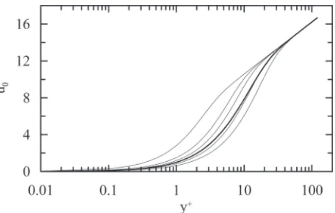
The mean and instantaneous velocity profiles for p+ = 0 are shown in Fig. 1. The logarithmic behavior

of all profiles for large y+ must be observed. Since all instantaneous profiles are required to tend to the same

steady solution for large y+, their average is objectively that solution. For small values of y+ solutions are

dominated by the error function, erf, for large y+ solutions are dominated by the special function, Ξ_.

To find parameters A0, t+

0 and T+B the software MathematicaTM was used. Solutions were found with 25

precision digits. Given the above four constrains, the feasible domain of Walker et al.'s model was found to

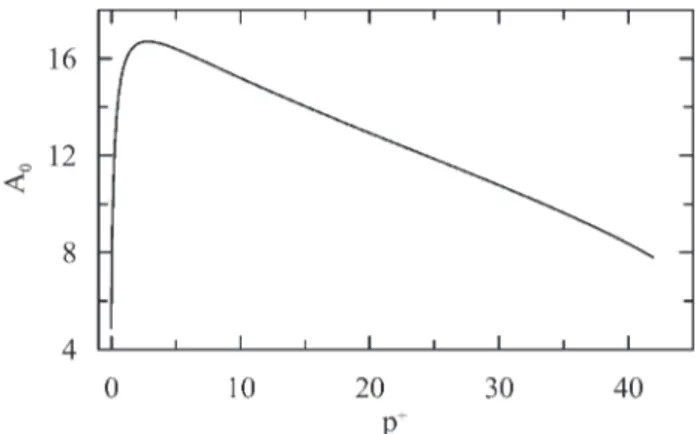
be p+2 [-0.025, 41.886]. The behavior of _A0, _t+₀ and _T+_B is shown in Figs. 2 and 3.

The behavior of A0 was not disclosed in Walker et al. (1989). This parameter appears in the integration

of Eq. (18). Basically, A0 controls the level of function erf. The process is non-linear and difficult to explain,

but generally as p+ increases, the last term in Eq. (23) becomes large and negative. The other terms of the

equation must then counterbalance this effeect to keep the global level of the external logarithmic solution in accordance with the classical law of the wall. The discussion is further aggravated by the realization that the relative magnitude of the terms in Eq. (23) vary with time during a cycle. Consider then the situation at

the end of a cycle, t+_/T+

B = 1. For p+ about three, the negative term achieves its maximum absolute value.

Also at about this value A0 achieves a maximum (Fig. 2). The contribution of the erf-term in Eq. (23) to counterbalance the pressure term reaches its maximum, with about 2/3 of the total contribution. The Ξ-term

becomes prevalent for p+ > 20.

Figure 1 - Mean (thick line) and instantaneous velocity profiles for p+ = 0 (t+/T +B= 0.01, 0.1, 0.2, 0.5, 1).

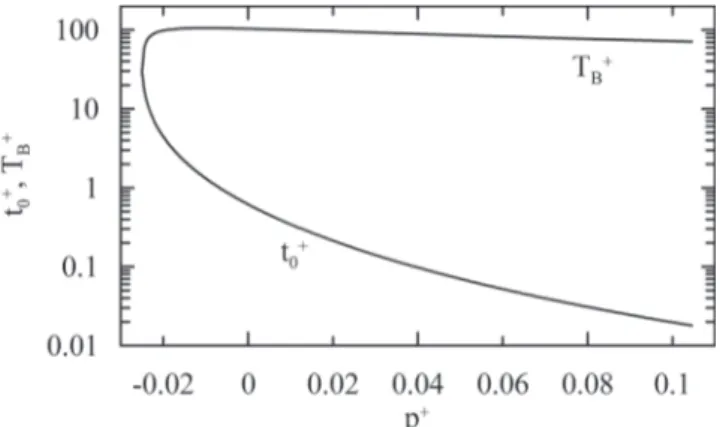
The characteristic behavior of t+0 and T+B at the extremes of the interval [-0.025, 41.886] where t+0 = T+B, are

devoid of physical meaning. Let alone the fact that these two time scales should be at least two orders of magnitude

stringency on the validity of the physical model, a second condition can be added; this is discussed below.

The lowest value of t+

0 is obtained for p+ = 2.9 (= 0.000058).

In the physical model formulation, the instantaneous and mean velocity profiles are always required to approach a logarithmic solution in the outer region. Velocity logarithmic profiles are typical of attached

flows. Once separation occurs, a different velocity profile of the type y1/2 sets in (Stratford (1959), Loureiro

and Silva Freire (2009, 2011), Loureiro et al. (2008)). Even over rough surfaces a y1/2-profile is observed

for the mean velocity profile at a separation point (Loureiro et al. 2009).

In Walker et al. (1989), instantaneous and averaged velocity profiles are presented for four combinations

of p+ and T+B in accordance with typically measured values. For constant pressure flow (p+ = 0.0, T+B = 110.2)

the canonical boundary layer structure is well reproduced. Under a favorable pressure gradient (p+ = ‒

0.098, T+B = 164), the instantaneous profiles are accelerated as expected. For adverse pressure gradients

(p+ = 0.11, _T+

B = 29.8; p+ = 0.5, T+B = 25), T+B decreases and, for the latter case, reverse instantaneous flow

is observed over the latter portion of the cycle.

In our computations, the second set of conditions (p+ = ‒ 0.098) could not be reproduced since

some of the flow parameters were rendered imaginary numbers. All other flows were well reproduced,

including the instantaneous reverse flow for condition p+ = 0.5 (Fig. 4). However, for _p+ = 0, Walker et

al. (1989) found ( t+0 = 0.008, T+B = 110.2), whereas we have found ( t+0 = 0.62, T+B = 103.4).

Figure 2 - Characteristic behavior of A₀.

Figure 4 - Mean (thick line) and instantaneous velocity profiles for p+ = 0.5 (t+ / T+B = 0.01, 0.1, 0.2, 0.5, 1).

In the instantaneous motion equations, scale velocities were introduced in terms of the friction velocity,

Eq. (4). As defined in Walker et al. (1989), u_τ is obtained from the time-mean structure, which is never

allowed to admit a y1/2 behavior for the mean-velocity profile irrespective of the value of p+; as a corollary,

u_τ is also never admitted to be negative or zero. However, in an unsteady flow computation, if at two distinct

instants of time the instantaneous velocity derivatives at the wall change sign, there must be a third instant where it is identical to zero. At this instant, the wall scaling variables need to be expressed in terms of the local pressure gradient at the wall. In fact, close to a separation point the relevant velocity scale in the wall region is upv(= (v/p)(

@

@

negative velocity derivatives at the wall must not be allowed to occur.

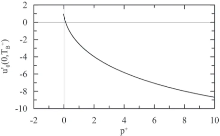
To determine the pressure gradient value where flow separation is first observed, consider the extreme

situation, t+ = T+B , that is, the end of the cycles. Figure (5) shows that du0 / dy+ = 0 at p+ = 0.104996.

Therefore, if as a further requirement, the model of Walker et al. (1989) is asked to furnish only positive

derivatives at the wall for the instantaneous velocity, the feasible domain is reduced to p+ 2 [-0.025,

0.104996]. The behavior of parameters A0, t+

0 and T+B can then be better observed in Figs. 6 and 7.

Figure 5 - First derivative of Eq. (23) at the wall and at t+ =T+B as

Figure 6 - Characteristic behavior of A0 with the extra condition

u'0 (y = 0) > 0.

Figure 7 - Characteristic behavior of t +₀ and T +_B with the extra condition u'₀ (y = 0) > 0.

Figure (7) shows that if a fourth condition is considered, that is, ord( t+0/T+B) = 103, the feasible domain

is reduced further to p+₂ [-0.005, 0.104996]. Of course, this is an arbitrary condition based on experimental

information. However, it does illustrate how Fig. (7) can be used to determine a domain of validity to the model of Walker et al. (1989) that is physically meaningful.

FINAL REMARKS

The present work has discussed for the first time the domain of validity of the unsteady wall-layer model of Walker et al. (1989) for the velocity profile in turbulent flows.

The model is formulated in terms of some very general considerations on the observed coherent motions in the wall region. However, after many simplifications, the flow features are expected to be represented by a nonhomogeneous time-dependent, one-dimensional, diffusion equation. Effects due to the structure of the organized motions are then restricted to the specification of the duration of a cycle and to the prescription of the external pressure gradient. Despite a claim from the original authors, the model is not appropriate to describe transient reverse flows.

(Mikhailov and Silva Freire 2012). Real time simulators for the velocity profile were implemented and can be obtained from either authors.

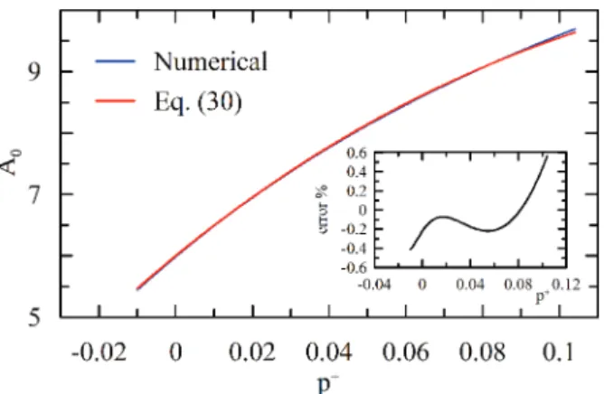
Provided a flow representation is required in the interval p+ ₂ [-0.010, 0.104496], the following

parameterization can be used:

(30)

A0 = A03(p+)3 + A02(p+)2 + A01p+ + A00

with A03 = 260.0, A02 = -177.7, A01 = 51.3, A00 = 6.0 and a maximum relative error of 0.5% (Figure 8);

(31)

T+

B = TB2(p+)2 + TB1p++ TB0

with TB2 = 719.0, TB1 = -383.7, TB0 = 103.1 and a maximum relative error of 1.5% (Figure 9);

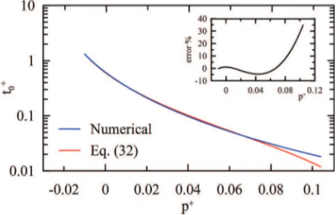
t+ 0=

t01

+ t00 ( t02+ (p+))2

(29)

with t01 = 0.000646, t02 = 0.0319, t00 = -0.0231.

Figure 8 - Parameterization of A₀ in the interval p+ 2 [-0.010, 0.104496], (Eq. 30). Error % stands for 100(A_0numerical ‒ A_0approximate)/A_0numerical .

Figure 9 - Parameterization of T+B in the interval p +

Because the values of t+0 span three orders of magnitude, and in view of the low values that this

parameter attains as p+ → 0.104496, it was difficult to find a simple fit that furnished good results for the

whole interval. At the extreme right, the relative error given by Eq. (32) is about 30% (Figure 10). However,

over much of the interval, p+₂ [-0.010, 0.075], the relative error is below 5%. In any case, equations (11)

and (23) show that the impact of a large relative error in t+0 on the evaluation of u0 is very small.

The set of Eqs. (23) and (30) through (32) permits a straightforward implementation of the model of Walker et al. (1989) in a domain that has physical meaning.

Figure 10 - Parameterization of t+0 in the interval p

+_{2 [-0.010,}

0.104496], (Eq. 30). Error % stands for 100(T0numerical ‒

T0approximate)/T0numerical .

ACKNOWLEDGMENTS

MDM is thankful to the Conselho Nacional de Desenvolvimento Científico e Tecnológico (CNPq) and the Instituto Nacional de Metrologia, Qualidade e Tecnologia (INMETRO) for their financial support of this research through a CNPq Research Fellowship - Edital MCT/CNPq/Inmetro no 059/2010 - PROMETRO, process No 563061/2010-3. APSF is grateful to the Conselho Nacional de Desenvolvimento Científico e Tecnológico (CNPq) for the award of a Research Fellowship (Grant No 303982/2009-8). The work was financially supported by the Fundação Carlos Chagas Filho de Amparo à Pesquisa do Estado do Rio de Janeiro (FAPERJ) through Grant E-26/102.937/2011.

RESUMO

O presente trabalho estuda em detalhe o modelo parietal transiente de Walker et al. (1989, AIAA J., 27, 140-149) para perfis de velocidade em escoamentos turbulentos. Dois novos termos são adicionados ao sistema transcedental não linear de equações que é utilizado para determinar os três principais parâmetros do modelo. Os domínios matemático e físico de validade do modelo são determinados como uma função do parâmetro gradiente de pressão adimensional

(p+). Uma parametrização explícita em termos de p+ é apresentada para o período médio entre eventos (T+

B), para a

origem do tempo (t+

0) e para a constante de integração (A0) da equação dependente do tempo. Na presente análise,

todos os sistemas de equações diferenciais são transformados, resultando em um procedimento computacional rápido que pode ser utilizado para o desenvolvimento de simuladores em tempo real.

REFERENCES

BARK FH.1975. On the wave structure of the wall region of a turbulent boundary layer. J Fluid Mech 70: 229-250.

BUSH WB AND FENDELL FE. 1972. Asymptotic analysis of turbulent channel flow and boundary-layer flow. J Fluid Mech 56: 657. CHAPMAN DR AND KUHN GD. 1986. The limiting behaviour of turbulence near a wall. J Fluid Mech 170: 265-292.

COLES D. 1956. The law of the wake in turbulent boundary layers. J Fluid Mech 1: 191-226.

CRUZ DOA AND SILVA FREIRE AP. 1998. On single limits and the asymptotic behaviour of separating turbulent boundary layers. Int

J Heat and Mass Transfer 41: 2097-2111.

GAD-EL-HAK M AND BANDYOPADHYAY PR. 1994. Reynolds number effects in wall-bounded turbulent flows. Appl Mech Review

47: 307-365.

GOLDSTEIN S. 1930. Concerning some solutions of the boundary layer equations in Hydrodynamics. Proc Cambridge Phil Soc 26:

1-18.

GOLDSTEIN S. 1948. On laminar boundary-layer flow near a position of separation. Q J Mech Appl Maths 1: 43-69.

HATZIAVRAMIDIS DT AND HANRATTY TJ. 1979. The representation of the viscous wall region by a regular eddy pattern. J Fluid

Mech 95: 655-679.

HSIEH K-J, LIEN F-S AND YEE E. 2010. Towards a unified turbulence simulation approach for wall-bounded flows. Flow Turbulence

Combustion 84: 193-218.

KLINE SJ, REYNOLDS WC, SCHRAUB FA AND RUNDSTADLER PW. 1967. The structure of turbulent boundary layers. J Fluid Mech

30: 741-773.

LANDAHL MY. 1990. On sublayer streaks. J Fluid Mech 212: 593-614.

LAUFER J. 1954. The structure of turbulence in fully developed pipe flow. (NACA Report no. 1174, 1954).

LOUREIRO JBR, MONTEIRO AS, PINHO FT AND SILVA FREIRE AP. 2008. Water tank studies of separating flow over rough hills",

Boundary-Layer Meteorol 129: 289-308.

LOUREIRO JBR, MONTEIRO AS, PINHO FT AND SILVA FREIRE AP. 2009. The effect of roughness on separating flow over

two-dimensional hills. Exp Fluids 46: 577-596.

LOUREIRO JBR AND SILVA FREIRE AP. 2009. Note on a parametric relation for separating flow over a rough hill", Boundary-Layer

Meteorol 131: 309-318.

LOUREIRO JBR AND SILVA FREIRE AP. 2011. Scaling of turbulent separating flows. Int J Eng Sci 49: 397-410.

MELLOR GL. 1966. The effects of pressure gradients on turbulent flow near a smooth wall. J Fluid Mech 24: 255-274.

MELLOR GL. 1972. The large Reynolds number, asymptotic theory of turbulent boundary layers. Int J Eng Sci 10: 851-873.

MIKHAILOV MD AND SILVA FREIRE AP. 2012. The Walker function. Math J 14: 1-9.

MILLIKAN CB. 1939. A critical discussion of turbulent flow in channels and tubes. in Proc. 5th Int. Congress on Applied Mechanics

(J Wiley, N.Y, 1939).

NICKELS TB. 2004. Inner scaling for wall-bounded flows subject to large pressure Gradients. J Fluid Mech 521: 217-239.

PATANKAR SV AND SPALDING DB. 1967. Heat and Mass Transfer in Boundary Layers. (Morgan-Grampian Press, London.

PIOMELLI U AND BALARAS E. 2002. Wall-layer models for large-eddy simulations. Ann Rev Fluid Mechanics 34: 349-374.

PRANDTL L. 1925. Über die ausgebildete Turbulenz. ZAMM 5: 136-139.

STRATFORD BS. 1959. The prediction of separation of the turbulent boundary Layer. J Fluid Mech 5: 1-16.

SYCHEV VV AND SYCHEV VV. 1987. On turbulent boundary layer structure. P.M.M. U.S.S.R 51: 462-467.

VON KARMAN TH. 1930. Mechanische aehnlichkeit und turbulenz, in Proc. Third Intern. Congress for Appl. Mech. Stockholm.

WALKER JDA AND ABBOTT DE. 1976. Implications of the structure of the viscous wall layer, in Turbulence in Internal Flows.

Edited by. Murthy SNB (West Lafayette, 1976), p. 131.

WALKER JDA, ABBOTT DE, SCHARNHORST RK AND WEIGANDG G. 1989. Wall-layer model for the velocity profile in turbulent flow.

AIAA J 27: 140-149.

WOLFRAM RESEARCH. 2008. Mathematica, Technical and Scientific Software, http://www.wolfram.com.