Stochastic Processes and Queueing Theory used in Cloud Computer Performance Simulations

Stochastic Processes and Queueing Theory used in Cloud Computer

Performance Simulations

Florin-Cătălin ENACHE

Bucharest University of Economic Studies catalin.enache@live.com

The growing character of the cloud business has manifested exponentially in the last 5 years. The capacity managers need to concentrate on a practical way to simulate the random demands a cloud infrastructure could face, even if there are not too many mathematical tools to simulate such demands.This paper presents an introduction into the most important stochastic processes and queueing theory concepts used for modeling computer performance. Moreover, it shows the cases where such concepts are applicable and when not, using clear programming examples on how to simulate a queue, and how to use and validate a simulation, when there are no mathematical concepts to back it up.

Keywords: capacity planning, capacity management, queueing theory, statistics, metrics

Introduction During the last years, the types and complexity of people’s needs increased fast. In order to face all changes, the technology had to develop new ways to fulfill the new demands. Therefore, I take a deeper look into the basic terms needed for understanding the stochastic analysis and the queueing theory approaches for computers performance models. The most important distribution for analyzing computer performance models is the exponential distribution, while the most representative distribution for statistical analysis is the Gaussian (or normal) distribution. For the purpose of this article, an overview of the exponential distribution will be discussed.

2.1 The Poisson Process

In probability theory, a Poisson process is a stochastic process that counts the number of events and the time points at which these events occur in a given time interval. The time between each pair of consecutive events has an exponential distribution with parameter λ and each of these inter-arrival times is assumed independent of other inter-arrival times. Considering a process for which requests arrive at random, it turns out that the density function that describes that random process is exponential. This derivation will turn out

to be extremely important for simulations, in particular for applications modeling computer performance. A typical example is modeling the arrival of requests at a server. The requests are coming from a large unknown population, but the rate of arrival,λ can be estimated as the number of arrivals in a given period of time. Since it is not reasonable to model the behavior of the individuals in the population sending the requests, it can be safely assumed that the requests are generated independently and at random.

Modeling such a process can help answering the question of how a system should be designed, in which requests arrive at random time points. If the system is busy, then the requests queue up, therefore, if the queue gets too long, the users might experience bad delays or request drops, if the buffers are not big enough. From a capacity planner point of view, it is important to know how build up a system that can handle requests that arrive at random and are unpredictable, except in a probability sense.

To understand and to simulate such a process, a better understanding of its randomness is required. For example, considering the following time axis (as in the second figure), the random arrivals can be represented as in the figure below.

Fig.1. Random arrivals in time

If X is the random variable representing the times between two consecutive arrivals (arrows), according to the PASTA Theorem(Poisson Arrivals See Time Averages)[1], it is safe to assume that all

X-es are probabilistically identical. Describing this randomness is equivalent to finding the density function of X that represents the time distance between two consecutive arrows.

Fig.2.Interval of length divided into n intervals.

The problem described above needs to be transformed so that it can be handled with known mathematical tools. Supposing that an arbitrary interval of length is chosen, then the probability of the time until the first arrival is longer than is P(X> ). This is by definition 1-FX( ), where FX( )

is the distribution function to be calculated. If time would be discrete, by dividing the interval between 0 and into n intervals, the calculating FX( ) reduces to

calculating the probability of no arrow in the first n intervals, and switching back to the continuous case by taking n→ ∞. Let p be the probability that an arrow lands in any of the n time intervals, which is true for any of the n intervals since any of them is as likely as any other to have an arrow

in it, then P X( > = −t)

(

)

the probability on no arrow, 1-p, in the first n intervals. As mentioned, when taking n→ ∞ , p→0+andnp=λt. The equality np=λt represents the average number of arrows in n intervals – np – which is equal to the average number of arrows calculated as λt - the arrival rate

multiplied by the length of the

interval.After switching to the continuous case, it is derived that:

0

0 _{lim 1}

( ) lim(1 ) lim(1 )

n x n

n n t

n n

t x

p _e

np t _n

t

P X t p e

n

λ

λ

λ

+

→∞

−

→∞ →∞

>  

→ _{+ =}

=  

> = − = − ========₁₄₂₄₃

(1) Which is equivalent to

0, ( 0)

( ) 1 ( )

1 t, ( 0)

t P X t P X t

e−λ t

<



≤ = − > =

− ≥



and ( ) ( ) 0, ( 0)

, ( 0)

X X t

t d

f t t

dtF λe−λ t

<



= =

≥

 (2)

2.2 The exponential distribution.

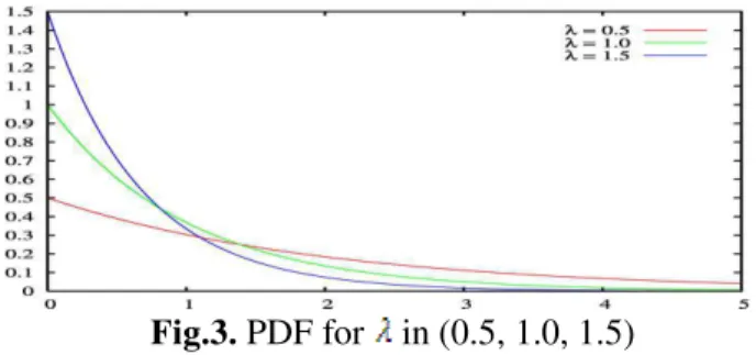
The random variable X derived from the Poisson process studied in section 2.1 of this paper is called exponential with the parameter ( X~Exp( ) ).The probability density function(PDF) of X is defined as

fX ( )= , which plots as in the

Fig.3. PDF for in (0.5, 1.0, 1.5)

Integrating by parts,it is easy to demonstrate the property that

0

1

t e λdt λ

∞

− ₌

∫

, which is actually obvious, since the sum of all probabilities of a random variable X has to add up to 1.If X~Exp( ) then the following properties are true[2] :

• The expected value the random

variable X,

E(X)=

0

1

t t eλ λdt

λ

∞

− ₌

∫

• Expected value of X2 ,

E(X2)= 2 ₂

0

2

t t λe λdt

λ

∞

− ₌

∫

• The variance of X, V(X)=E(X2) –

[E(X)]2=

2

2 2

2 1 1

λ λ λ

 

−  =

  (5) .

When used in simulating computer performance models,the parameter λ denotes usually the arrival rate. From the properties of the exponential distribution, it can be deduced that the higher the arrival rate λ is, the smaller are the expected value – E(X) – and variance – V(X) – of the exponentially distributed random variable X.

3.1. Introduction to the Queueing

Theory M/G/1 Problem – FIFO

Assumption

Considering a system where demands are coming are random, but the resources are limited,the classic queueing problem is how to describe the system as a function of random demands. Moreover, the service times of each request are also random, as

in figure 4:

Fig. 4. Random arrivals with random service times

From a request point of view, when a new request arrives, it has two possibilities:

• It arrives and the server is available. Then it keeps the server busyfor a random amount of time until the request is processed, or

• Typical case, when a request arrives, it finds a queue in front of it, and it needs to wait.

was in service at the time of the arrival of the current request.

Calculating the expected waiting time of the new requestmathematically, it would be the sum(further named “convolution”) of the density functions of each of the service time requirements of the requests in the queue, which could be any number of convolutions, plus the convolution with the remaining partial service time of the customer that was in service at the time of the arrival of the current request. Furthermore, the number of terms in the convolution, meaning the number of requests waiting in the queue, is itself a random variable[1].

On the other side, looking at the time interval between the arrival and the leave of the nthrequest, it helps in developing a recursive way of estimating the waiting times. The nthrequest arrives at time Tn

and, in general, it waits for a certain amount of time – noted in the below figure with Wn. This will be 0 if the request

arrives when the server is idle, because the request is being served immediately. To enforce the need of queueing theory, in real-life, a request arrives typically when the server is busy, and it has to wait. After waiting, the request gets serviced for a length of time Xn , and then leaves the

system.

Fig. 5. Representation for calculating the waiting time, depending on the arrival of the (n+1)th customer

Recursively, when the next customer arrives, there are 2 possibilities:

• The arrival can occur after the nthrequest was already serviced, therefore Wn+1=0 (explained in the

right grey-boxed part of figure 5), or

• The arrival occurs after Tn but

before the nth request leaves the system. From the fifth figure the

waiting time of the (n+1)th request is deduced as the distance between its arrival and the moment when the nthrequest leaves the system, mathematically represented as Wn+1=Wn+Xn-IAn+1, where IAn+1is

the inter-arrival time between the nth and (n+1)threquest.This can be easily translated into a single instruction that can be solved recursively using any modern programming language.

3.2. Performance measurements for the M/G/1 queue

If λ is the arrival rate and X is the service time, the server utilization is given by:

( ), ( ) 1

1,

E X if E X

otherwise

λ λ

ρ= <

 (6)

Moreover, if the arrivals are described by a Poisson process, the probability that a request must wait in a queue is

(

)

P W > =ρ(7) , and the mean waiting time is given by the Pollaczek-Khintchin formula[3] :

( )

( ) ( )

* (1 )

1 2 ( )

E X V

E W X

E X ρ

ρ

= +

− ₍₈₎

of the waiting time is given by the following formula[1]:

(1 ) ( )

0, 0

( )

1 , 0

t

W p

E X t

F t

e t

ρ − −

<

 

=

 _{− ≥}

 ₍₉₎

There is no simple formula for Fw(t)when the service times are not exponentially distributed, but using computer simulation can help developing such models, after validating classic models as the one above.

4.1. Software simulation of the Queueing Problem

As described previously, modeling the M/G/1 queue can be done by using a recursive algorithm by generating the inter-arrival time and the service times using the Inverse Transform Method[4]. The following lines written in the BASIC programming language simulate such an

algorithm, although almost any

programming language could be used.

100 FOR I=1 to 10000

110 IA= ‘inter-arrival times to be generated 120 T=T+IA ‘time of the next arrival

130 W=W+X-IA ‘recursive calculation of waiting times 140 IF W<0 THEN W=0

150 IF W>0 THEN C=C+1 ‘count all requests that wait 160 SW=SW+W ‘sum of waiting times for calculating E(W) 170 X= ‘service times to be generated

180 SX=SX+X ‘sum of service times for calculating Utilization 190 NEXT I

200 PRINT SX / T, C / 10000, SW / 10000 ‘ print Utilization, P(W) and E(W)

4.2. Generating random service and inter-arrival times using the Inverse Transform Method

Assuming that the computer can generate independent identically distributed values that are uniformly distributed in the interval (0,1), a proper method of

generating random variable values

according to any specified distribution function is using the Inverse Transform Method.

To generate the random number X, it is enough to input the randomcomputer generated number on the vertical axis

andto project the value over the

distribution function G, where G is the desired

distribution to be generated. Projecting the point from the G graph furtherdown on the horizontal axis, delivers the desired randomly distributed values described by the G density function.This method is practically reduced to finding the inverse function of the distribution function of the distribution according to which the numbers are generated.By plugging in the computer randomly generated numbers, a new random variable is generated with has its distribution function G(u) [4]. This procedure is schematically described in the below figure.

For example, for a Poisson process of arrivals that are exponentially distributed with parameter λ, where λ is the arrival

rate and 1 E IA( )

λ = , according to the

Inverse Transform Method, a value of λ=1.6 arrivals per second is derived, equivalent to anaverage inter-arrival time

of 1 5

8

λ = seconds. For

( ) 1 u

G u = −λe−λ =R with u≥0, it is

deduced that 1

( ) 1 / ln(1 )

G− R = − λ −R

where R is the computer generated value. Therefore, the instruction 110 from section 3 of this paper becomes:110 IA=-(5/8)*LOG(1-RND), where RND is the BASIC function that generate values uniformly distributed between 0 and 1.Of course, any programming language that is able to generate random independent identically distributed numbersbetween 0 and 1 can be used for simulation.

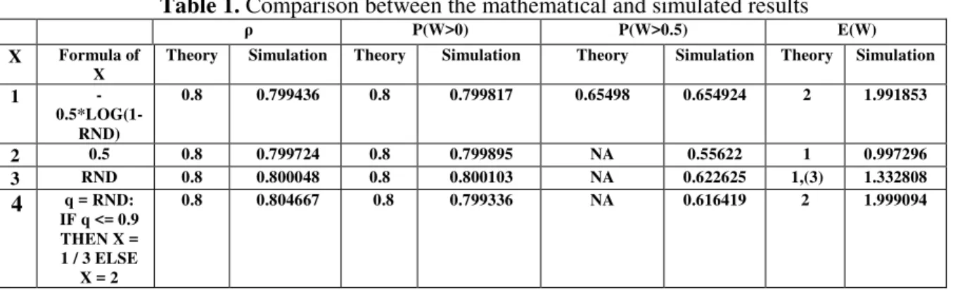
5. Comparing the mathematical solution of the queueing problemwith the computer simulation

To illustrate the applicability of the software simulation, 4 different arrival times distributions are analyzed :

1. Exponential service time, with

mean service time E(X)=0.5

2. Constant service time, X=0.5

3. Uniformly identical distributed

service times between 0 and 1, X~U(0,1)

4. Service times of 1/3 have a

probability of 90%,and service times of 2 have a probability of 10%.

For all 4 simulations, exponential

distributed inter-arrivals with λ=1.6 are used as derived in 4.2 section. All calculations in the following table are done according to the formulas presented in section 3.2.

Table 1. Comparison between the mathematical and simulated results

ρ P(W>0) P(W>0.5) E(W)

X Formula of X

Theory Simulation Theory Simulation Theory Simulation Theory Simulation

1

- 0.5*LOG(1-RND)

0.8 0.799436 0.8 0.799817 0.65498 0.654924 2 1.991853

2 0.5 0.8 0.799724 0.8 0.799895 NA 0.55622 1 0.997296

3 RND 0.8 0.800048 0.8 0.800103 NA 0.622625 1,(3) 1.332808

4 q = RND: IF q <= 0.9 THEN X = 1 / 3 ELSE

X = 2

All 4 simulations have been chosen in such way that E(X)=0.5, and the distinction is done by choosing the service times with different distributions. Since the utilization is directly dependent on the arrival rate and mean arrival times, it is equal with 80% in all 4 cases. According to (7), the probability of waiting is also equal to 80% in all 4 cases.

In this simulation, the mean waiting time, as deduced from the Pollaczek-Khintchin(8) formula, confirms the accuracy of the simulation model, and gives insights also for the other cases, offering a clear approximation of the behavior of the designed system. It is interesting to observe that mean waiting time when having exponential service times is double in comparison with the mean waiting time when having constant service times, although the mean service time, the utilization and the probability of waiting are equal in both cases.

6. Conclusions

Based on all information presented in this paper, I can conclude that computer simulation is an important tool for the analysis of queues whose service times have any arbitrary specified distribution. In addition, the theoretical results for the special case of exponential service times(8) are extremely important because

they can be used to check the logic and accuracy of the simulation, before extending it to more complex situations. Moreover, such a simulation gives insight on how such a queue would behave as a result of different service times. Further, I consider that it offers a methodology for looking into more complicated cases, when a mathematical approach cannot help.

References

[1] R. B. Cooper, Introduction to Queueing Theory, Second Edition. New York: North Holland, 1981, pp. 208-232.

[2]S. Ghahramani, Fundamentals of Probability with Stochastic Processes, Third Edition. Upper Saddle River, Pearson Prentice Hall 2005, pp.284-292. [3] L. Lakatos , “A note on the Pollaczek-Khinchin Formula”, Annales Univ. Sci. Budapest., Sect. Comp. 29 pp. 83-91, 2008.

[4]K. Sigman, “Inverse Transform Method”. Available :

http://www.columbia.edu/~ks20/4404-Sigman/4404-Notes-ITM.pdf [January 15, 2015].

[5] K. Sigman, “Exact Simulation of the stationary distribution of the FIFO M/G/c Queue”, J. Appl. Spec. Vol. 48A, pp. 209-213, 2011, Available :

http://www.columbia.edu/~ks20/papers/Q UESTA-KS-Exact.pdf [January 20, 2015]