The equity risk premium and the
low frequency of the term spread
International Evidence
Ana Isabel Oliveira Novais
Católica Porto Business School March 2019
The equity risk premium and the
low frequency of the term spread
International Evidence
Final Assignment in the modality of Dissertation presented to Universidade Católica Portuguesa to obtain the degree of Master in Finance
by
Ana Isabel Oliveira Novais
under the supervision of
(PhD) Gonçalo Faria and (PhD) Fabio Verona
Católica Porto Business School March 2019
Acknowledgments
I would like to thank everyone that supported me during my thesis period. Especially, I would like to thank to my supervisors, Professor Gonçalo Faria and Professor Fabio Verona, who helped me to surpass all technical questions and for all the knowledge transmitted and my parents, who always supported me on this project and provided me everything that I needed.
I also would like to thank my closest friends and family for all the support and motivation provided.
Resumo
Nesta tese analisamos o poder de previsão out-of-sample do term-spread e dos seus domínios de frequência sobre prémios de risco de mercado. A variável term spread representa a diferença entre taxas de juro de longo e curto prazo de obrigações do governo e a sua decomposição em domínio de frequência é feita através do método Maximum Overlap Discrete Wavelet Transform.
Foi comprovado pela literatura que no mercado dos Estados Unidos da América a componente de baixa frequência do term spread tem uma performance forte e robusta em exercícios out-of-sample sobre prémios de risco de mercado. Nesta tese, abordamos a possibilidade de este indicador ter a mesma performance em mercados internacionais (Alemanha, França, Japão, Reino Unido, Canada, África do Sul e Australia). Até então, esta alternativa ainda não foi abordada na literatura, e consideramos muito importante a sua análise para os mais diversos investidores, tanto locais como internacionais.
A principal conclusão desta tese é que a série original em domínio temporal e a componente de baixa frequência do term spread tem uma performance out-of-sample forte e robusta a prever prémios de risco de mercado para além dos Estados Unidos da América, na Alemanha, na França e no Canada.
Palavras-chave: Prémio de Risco de Mercado, Term Spread, Domínio de Frequência
Abstract
In this thesis we analyze the equity risk premium out-of-sample forecasting power of the term spread and its frequency components. The term spread is the difference between long and short term governmental interest rates and its frequency decomposition is done by applying a Maximum Overlap Discrete Wavelet Transform approach.
It has been shown in the literature that, in the United States of America equity market, the low frequency of the term spread is a strong and robust out-of-sample predictor of equity risk premium. In this thesis we address the empirical question if in alternative geographic zones (Germany, France, Japan, United Kingdom, Canada, South Africa and Australia) that continues to be the case.
This question has not been addressed so far in the literature and we foresee it as highly relevant for both local and international diversified equity investors.
Our main conclusion is that the original time series and the low frequency component of the term spread are a strong and robust out-of-sample predictors of the equity risk premium beyond United States of America, namely in Germany, France and Canada.
Index / Contents
Acknowledgments ... V Resumo ... VII Abstract ... IX Index / Contents ... XI Introduction ... 20 Literature Review ... 241.1 Forecasting Equity Risk Premium ... 24
1.1.1 Out-of-Sample Forecast ... 28
1.1.2 International Evidence ... 29
1.2. Frequency Domain Analysis And Wavelet Methods ... 30
Data And Methodology ... 34
2.1 Data ... 34
2.2 Method ... 37
2.2.1 Wavelet Methods ... 37
2.2.1.1. Maximal Overlap Discrete Wavelet Transform Multiresolution Analysis (MODWT MRA) 40 Empirical Results ... 45
3.1 Frequency Components Of The Term Spread ... 45
3.2 In-Sample Forecasting ... 49
3.2.1 Results ... 50
3.2.1.1 – Germany ... 50
3.2.1.2 – France ... 51
3.2.1.3 – Japan... 51
3.2.1.4 – United States of America ... 52
3.2.1.5 – United Kingdom ... 52 3.2.1.6 – Canada ... 53 3.2.1.7 – South Africa ... 53 3.2.1.8 – Australia ... 54 3.3 Out-Of-Sample Forecasting ... 55 3.3.1 Analysis of Results ... 57 3.3.1.1 Germany ... 57 3.3.1.2 France... 58 3.3.1.3 Japan ... 58
3.3.1.4 United States of America ... 59
3.3.1.6 Canada ... 60
3.3.1.7 South Africa ... 60
3.3.1.8 Australia ... 61
3.3.2 – Cumulative sum of squared forecast errors ... 61
3.4 Robustness Analysis ... 66
3.4.1 Different Sample Periods ... 66
3.4.1 J=6 level MODWT MRA ... 71
Conclusion ... 75
Bibliography ... 77
List of Figures
Figure 1: Decomposition of Maximum Overlap Discrete Wavelet Transform
(Source: Matlab Tech Talks: Kirthi Devleker) ... 42
Figure 2: Time series of the term spread and of its different components for Germany... 46
Figure 3: Time series of the term spread and of its different components for France ... 46
Figure 4: Time series of the term spread and of its different components for Japan ... 46
Figure 5: Time series of the term spread and of its different components for U.S.A ... 47
Figure 6: Time series of the term spread and of its different components for U.K ... 47
Figure 7: Time series of the term spread and of its different components for Canada ... 47
Figure 8: Time series of the term spread and of its different components for South Africa ... 48
Figure 9:Time series of the term spread and of its different components for Australia ... 48
Figure 10: Cumulative sum of squared forecast errors for Germany ... 62
Figure 11: Cumulative sum of squared forecast errors for France ... 62
Figure 12: Cumulative sum of squared forecast errors for Japan ... 63
Figure 13: Cumulative sum of squared forecast errors for U.S. ... 63
Figure 14: Cumulative sum of squared forecast errors for U.K. ... 63
Figure 15: Cumulative sum of squared forecast errors for Canada ... 64
List of Tables
Table 1: Months captured by the oscillations of detail and smooth components
... 43
Table 2: In-Sample predictive regression results for Germany ... 50
Table 3: In-Sample predictive regression results for France ... 51
Table 4: In-Sample predictive regression results for Japan ... 51
Table 5: In-Sample predictive regression results for U.S. ... 52
Table 6: In-Sample predictive regression results for U.K ... 52
Table 7: In-Sample predictive regression results for Canada ... 53
Table 8: In-Sample predictive regression results for South Africa ... 53
Table 9: In-Sample predictive regression results for Australia ... 54
Table 10: Out-of-Sample R-squares for Germany ... 57
Table 11: Out-of-Sample R-squares for France ... 58
Table 12: Out-of-Sample R-squares for results for Japan ... 58
Table 13: Out-of-Sample R-squares for for U.S ... 59
Table 14: Out-of-Sample R-squares for U.K ... 59
Table 15: Out-of-Sample R-squares for Canada ... 60
Table 16: Out-of-Sample R-squares for South Africa ... 60
Table 17: Out-of-Sample R-squares for Australia ... 61
Table 18: Out-of-Sample R-squares of sub-samples for Germany ... 66
Table 19: Out-of-Sample R-squares of sub-samples for France ... 67
Table 20: Out-of-Sample R-squares of sub-samples for Japan ... 67
Table 21: Out-of-Sample R-squares of sub-samples for U.S.A ... 68
Table 22: Out-of-Sample R-squares of sub-samples for U.K ... 68
Table 23: Out-of-Sample R-squares of sub-samples for Canada ... 69
Table 25: Out-of-Sample R-squares of sub-samples for Australia ... 70 Table 26: Out-of-Sample R-squares computed with J=6 MODWT MRA for Germany... 71 Table 27: Out-of-Sample R-squares computed with J=6 MODWT MRA for France ... 71 Table 28: Out-of-Sample R-squares computed with J=6 MODWT MRA for Japan ... 72 Table 29: Out-of-Sample R-squares computed with J=6 MODWT MRA for U.S. ... 72
Table 30: Out-of-Sample R-squares computed with J=6 MODWT MRA for U.K ... 72
Table 31: Out-of-Sample R-squares computed with J=6 MODWT MRA for Canada ... 73 Table 32: Out-of-Sample R-squares computed with J=6 MODWT MRA for South Africa ... 73 Table 33: Out-of-Sample R-squares computed with J=6 MODWT MRA for Australia ... 73
Introduction
Forecasting Equity Risk Premiums (ERP) is a crucial input for investors in their process of dynamic portfolio adjustments. Additionally, an improved exercise of forecasting ERP plays a crucial rule in finance because it helps to understand some factors that command ERP and improve the ability to use more realistic asset pricing models.
Since a long time ago, the predictability of equity risk premiums has been an active research question for academic researchers (e.g., Dow (1920), Rapach and Zhou (2013)) and a very important topic in empirical finance.
The literature on this topic is very extensive and extremely difficult to embrace. Its majority is unanimous on the fact that ERP are predictable but is rather weak on the consensus about where does come from the forecasting power of the equity risk premium. Several studies in the last decades, have asked whether ERP can be predictable by macroeconomic variables such as dividend-price ratio, interest rate spread, consumption wealth ratio while other researchers focus on technical indicators to test this predictability. These predictors have been tested both in-sample (IS) and out-of-sample exercises (OOS) (e.g., Goyal and Welch 2008), although they have a very poor performance in out-of-sample exercises. Moreover, the extensive research on this topic is mostly dedicated to the United States (US) market.
In this paper we focus our analysis in the out-of-sample predictability of the equity risk premium given that in order to effectively predict ERP in real-time the out-of-sample exercise is the most suitable one.
We focus on one specific predictor: the spread between long and short governmental interest rates (term spread). We consider this variable very attractive once it is closely related with the business cycle1 and it is very easy to
compute using public available data. Furthermore, researchers as Campbell (1987) and Fama and French (1989), state that the term spread has predictability power over equity risk premiums, although the forecasting power of the term spread performs rather poorly when tested out-of-sample2, as it is the case of
many other variables. Being in line with that, we are particularly motivated by the findings of Faria and Verona (2018) which found out that the low frequency (long-term dynamics) of the term spread is a strong and robust predictor of the equity risk premium in out-of-sample exercises for the United States (U.S).
The major novelty of this thesis is that we extend this analysis beyond the U.S market to seven additional markets: Germany, France, Japan, United Kingdom, Canada, South Africa and Australia. This has not been addressed in the literature so far and we foresee it as highly relevant for both local and internationally diversified equity investors.
In line with that, the main research question is: “Is the original time series or any frequency component of the term spread a good out-of-sample predictor of the equity risk premium in international countries?”.
We closely follow the method used in Faria and Verona (2018) to test out-of-sample forecasting power of different frequency components of term spread over equity risk premiums. Using a frequency domain approach allow us to extract hidden information from the predictor that can be highly important to forecast
1 As it is showed by Wheelock and Wohar (2009) 2 See Goyal and Welch (2008)
ERP. Particularly, Ferreira and Santa Clara (2011) found that different frequency components of some indicators (earnings growth, dividend-price ratio) capture different frequencies of ERP. Similarly, Bandi, Perron, Tamoni, and Tebaldi (2018) and Faria and Verona (2018) succeeded on improving ERP predictability by having in account frequency components dependence between ERP and its predictors. The different frequency components of the term spread are computed using a Maximum Overlap Discrete Wavelet Transform method and are tested to forecast horizons of 1,3,6,12 and 24 months.
In this paper was found that the original time series and the low frequency component of the term spread have significant forecasting power on Germany, France, United States of America and Canada.
The dissertation is divided as follows: In Chapter 1 we provide a review on related stands of literature, while placing our contribution. In Chapter 2 is explained the data and the methodology. In Chapter 3 are presented the main results as well as a robustness analysis.
Chapter 1
Literature Review
Forecasting the equity risk premium has been in the mind of a lot of researchers in the last decades. Despite its extreme importance in Finance and the fact that many economists have tried to forecast ERP using different methods and predictors, the truth is that the predictability of this variable continues to motivate a lot of active research.
1.1 Forecasting Equity Risk Premium
Since the very beginning of the XX century, (e.g. Dow (1920)), the predictability of the equity risk premium has been an active research topic. This happens because the equity risk premium is a very important indicator for equity investors. The ERP tell us on an ex-ante basis how much additional return the investors demand as a premium for taking additional risks carried from stock ownership. Indeed, when we buy a stock its actual price is known, but investors do not know what expected returns are being priced on it. The equity risk premium offers an idea of how much is worth (or not) to invest on a stock against the alternative of investing in risk-free instruments.
As early as 1984, Rozeff (1984) explored the relationship between ERP and dividend yields, pointing out that “Stock market returns are not a random walk and that the current dividend yield provides a clue to future return
predictability.” According to his studies, as dividend yield increases, the stock market returns tends to move in the same direction.
Fama and French (1989) studied the relationship between expected returns on bonds and stocks. According to their research, the expected excess returns on stocks move together with expected excess returns on corporate bonds, which is in line with the fact that dividend yields, which are commonly used to forecast stock returns, are found to be also good predictors to forecast bond returns. Moreover, Fama and French (1989) share findings that associate other predictors to business cycles conditions. They specifically pointed out that the major movements in dividend yields and default spreads are connected to long term business conditions, whereas the term spread is associated to shorter business cycles. The term spread exhibits lower values across business-cycle peaks and higher values around troughs.
Martin Lettau and Sydney Ludvigson (2001) debated “whether expected returns vary at cyclical frequencies and with macroeconomic variables” arguing that returns are predictable because they represent a rational response of economic agents to economic conditions driven by risk aversion and by time-varying investment opportunities, against the hypothesis of inefficient markets. Following this idea and assuming that markets are efficient, it is reasonable to believe that macroeconomic variables occupy an important position concerning the prediction of stock returns.
Many more studies consider these and other macroeconomic variables to predict ERP, including nominal interest rate and interest rate spread (Keim and Stambaugh 1986, Campbell 1987, Fama and French 1989), inflation rate (Nelson 1976, Fama and Schwert 1977, Campbell and Vuolteenaho 2004), consumption wealth ratio (Lettau and Ludvigson 2001), dividend yield ( Rozeff 1984, Campbell and Shiller 1988, Fama and French 1988, Campbell and Yogo 2006,), price-earnings ratio (Campbell and Shiller 1988, …), among others.
Nevertheless, the predictors of the equity risk premium considered in the literature are not limited to macroeconomic variables. Some researchers proposed the inclusion of technical indicators.
As stated by Pring (2002): “The technical approach to investment is essentially a reflection of the idea that prices move in trends that are determined by the changing attitudes of investors toward a variety of economic, monetary, political, and psychological forces.” Research on technical analysis in this topic has received less attention, although it is possible to identify the study of trading strategies based on some technical indicators, for example, Fama and Blume (1966) proposed filter rules, Conrad and Kaul (1998) introduced momentum and Brock, Lakonishok and LeBaron (1992) presented moving averages.
Neely, Rapach, Tu and Zhou (2014) analyzed the capability of technical indicators to directly predict equity risk premium and compared their performance with macroeconomic variables’ performance. Their findings support the existence of predictability power of both types of predictors, although they capture different information about the ERP. They argue that macroeconomic variables perform better in detecting increases in the equity risk premium near business cycle troughs and technical analysis is dominant when it comes to predicting declines in the equity risk premium near business cycle peaks, sustaining the inclusion of both indicators to better forecast stock returns. The fact is that macroeconomic variables and technical indicators are considered by part of the literature to have predictive power over the equity risk premium. Following Neely, Rapach, Tu and Zhou (2014) the economic explanation is based on asset pricing models: the changes on macroeconomic trends are tracked by macroeconomic variables and the time varying expected stock returns are mostly driven by the future state of the economy. Concerning technical indicators, the economic explanation is not so clear; four models exist
This dissertation reassess the equity risk premium predictability of the term spread by considering its different frequencies components. We start by running an in-sample analysis and then we move to an out-of-sample exercise which is the principal analysis.
Recently, on this continuous search for a good predictor of the ERP, Faria and Verona (2018) found that in the U.S market, the low frequency of the term spread performs very well on forecasting equity risk premiums and better than that, the predictor has greater levels of predictability both in-sample and out-of-sample exercises. We are particularly surprised by the performance of the term spread on their research and motivated by this conjecture we study the out-of-sample forecasting power of the term spread and its frequency components over ERP in international markets. The term spread represents the difference in interest rates between two sovereign bonds with different maturities. Usually this difference is the difference between long-term and short-term governmental interest rates, and it is a proxy for the slope of the yield curve.
A great deal of effort has been made in the last century in order to test expectation models about the term structure of interest rates, which states that the slope of the yield curve (difference between long-term and short-term rates) reflects the market forecast about the changes in interest rates. When the forward interest rate equals the expected future spot rate and thus the expectation hypothesis holds, it is reasonable to use the yield curve to anticipate market expectations concerning future states of the economy. Under this hypothesis, low current short-term spot rates and high long-term rates are a sign of future economic growth.
However, the expectations theory about the term structure of interest rates has been rejected by some researchers, such as Campbell and Shiller (1991).
In 1987, Campbell showed that the variables which have been used in the expectations model as proxies for risk premium on twenty-year treasury bonds
also predict excess stock returns, which is in line with the findings of Fama and French (1989): expected excess returns on corporate bonds and stocks move together.
Regarding the out-of-sample approach which is the main analysis of this thesis, we consider the most reasonable approach to use once it uses information available until the moment of forecasting to forecast, being that way a real-time forecasting.
Goyal and Welch (2008), instead of keep looking for another predictor or another method which could improve the results of forecasting ERP exercise, decided to test on in-sample and out-of-sample exercises all variables considered as good predictors of ERP in the literature. Their findings state that most of the variables perform poorly in out-of-sample exercises and as they say: “OOS, most models not only fail to beat the unconditional benchmark (the prevailing mean) in a statistically or economically significant manner but underperform it outright.” Later, Faria and Verona (2018) found out that the low-frequency of the term spread is a good predictor of ERP in out-of-sample exercises. This is very relevant because the indicators performing well out-of-sample are almost inexistent which is the reason why this thesis focus on this predictor, following Faria and Verona (2018) to international markets. In the next subsection is provided a very brief summary of the authors that used the out-of-sample approach to financial purposes
1.1.1 Out-of-Sample Forecast
A considerable number of recent papers use the out-of-sample approach to test the predictive performance of equity risk premiums, using variables such as book-to-market ratios, dividend-to-earnings, consumption-to-wealth ratios and term spread. Lettau and Ludvigson (2001), Campbell and Thomson (2007), and
Goyal and Welch (2003, 2004) argue that the variables purposed as predictors of future ERP do not provide predictive gains on in-sample exercises. They stated that “Our paper has systematically investigated the empirical real-world out-of-sample performance of plain linear regressions to predict the equity premium. We find that none of the popular variables has worked – and not only post-1990 … Our profession has yet to find a variable that has had meaningful robust empirical equity premium forecasting power, at least from the perspective of real-world investor.” Authors such as Campbell and Thomson (2007) disagree with Goyal and Welch’s opinion, arguing that by implementing some restrictions when constructing out-of-sample forecasts, strong evidence emerges in regard to the out-of-sample predictive power in excess stock returns.
1.1.2 International Evidence
The literature about the prediction of the equity risk premium is extensive, although it is mostly dominated by the U.S market. This paper is a contribution for the study of equity risk premium predictability in international markets, i.e., beyond U.S. market.
There are a few papers studying the predictability of equity risk premium in international markets. Asprem (1989) explored the relationship between stock indexes, asset portfolios and macroeconomic variables in ten European countries. The findings of this paper state that inflation, imports, interest rates and employment are inversely related to stock indexes. Campbell and Hamao (1992) explored the U.S and Japan markets and found that variables such as dividend-price ratio and interest rates help to forecast excess monthly returns in both countries.
More recently, Schemeling (2009) explored how consumer confidence affects expected stock returns in 18 industrialized countries, and concluded that when the sentiment is low, future stock returns tend to be higher and when an investor
sentiment is high the future stock returns tend to be low. McMillan and Wohar (2011) used sum of parts modeling method to study the predictability of ERP. They found that in Italy, UK, USA and Korea this approach outperforms the alternative models. Later, Kumar Narayan, Seema Narayan and Thuraisamy (2014) tested the predictability of excess stock return and found evidence of in-sample predictability for 15 countries. They used a mean variance investor framework and argued that investors, in most of these emerging markets countries, can make significant profits if they adopt dynamic trading strategies. Moreover, Jordan, Vivian and Wohar (2014) stated that “macro and technical indicators can (statistically) improve forecast accuracy and generate gains to investors; in contrast to the U.S. results, predictability in our sample of European countries exists in recent data.”
1.2. Frequency Domain Analysis and Wavelet Methods
Financial analysis is mainly based on time series3 methods, which can track
the movements of any variable that changes over time.
The most popular approach used to study time series is time domain analysis, which represents the analysis of the signals displayed by the times series with respect to time. Moreover, the time domain analysis allows the study of the temporal properties of a given economic variable whose records occur at one determined frequency. The problematic issue here is whenever the occurrences of the variable are not visible in just one frequency (which would be the original time-series), but they occur in several different frequencies (which only frequency domain approach is able to identify). Whenever this happens, the time domain approach is not able to correctly process all the information contained in
the time series. Multiscale features is an important item of financial time series which translates the several structures observed in the time series, each one occurring in a different time scale. At this point, it is important to mention the definition of frequency domain analysis as a complementary tool for time domain analysis, so as to surpass the issues that may occur with time domain as described earlier. In opposition to time domain, frequency domain focuses on the analysis of mathematical functions in respect to frequency rather than time and investigates the significance of the different frequency levels on the behavior of the variable. Put simply, the time domain illustrates the extent at which the signal varies over time, whereas the frequency domain represents the extent at which a signal resides within each certain frequency band over an interval of frequencies.
Wavelet analysis takes into account both approaches, as it has the capacity to decompose the time series in a group of sub-time series each one associated to a given time scale. Wavelet methods offer a different view for the researcher, working as a zoom tool on details and offer a larger picture of the features of the series. As pointed by Ranta (2010): “…with wavelet methods we are able to see both the forest and the trees.” They are regarded as very attractive since they allow us to break down economic activity in different frequency components and to study them separately. In other words, wavelets methods can be employed to study an indicator’s time evolution which depends on the interface of a mix of different frequencies components.
The Fourier transform is a traditional approach in the frequency domain analysis and possesses the capacity to show how much each frequency exists in the signal. However, it does not have the capacity to identify the moment in time when these frequencies exist because it uses constant length windows. This implies a great probability that the fixed time windows contain a large number of high frequencies cycles and a small number of low frequencies, preventing an adequate examination for all frequencies. On the other hand, the wavelet
transform supports windows of different size, improving the time resolution of the high frequencies and the frequency resolution of low frequencies. The reason for that is that high frequencies are better located in time, whereas the low frequencies are better located in frequency. Another big disadvantage of the Fourier transform is that it requires the time series to be stationary4, while
wavelets work well when it comes to non-stationary data. This fact is particularly relevant because numerous economic and financial time series are scarcely stationary. These methods allow gathering information about a phase (expansion or regression) or the length of a cycle (e.g. business cycle).
In recent decades, wavelet methods have become more popular in a considerable number of areas, such as geophysics, medicine and engineering.
In finance, some examples using wavelet’s methods are: Capobianco (2004) that uses wavelet methods to study Nikkei stock index data and argues that it matches perfectly on the analysis of financial data, Crowly and Lee (2005) which applied wavelet multiresolution analysis to analyze different frequency components of European business cycles and Gençay et al. (2001a) investigating the scaling properties of foreign exchange rates.
Chapter 2
Data and Methodology
The aim of this thesis is to analyze the out-of-sample predictability power of the equity risk premium by the term spread and of its different frequencies components in international markets.
A detailed description of the data and the method used will be presented in the following two sub-sections.
2.1 Data
The sample set covers eight countries: Germany, France, Japan, United States of America, United Kingdom, Canada, South Africa and Australia. We use monthly observations from March 1973 to August 2018 and data was gathered from DataStream database, Organization for Economic Cooperation and Development (OECD), Federal Reserve Economic Data (FRED) and International Monetary Fund (IMF). A more detailed description of the variables and their source is provided below.
• Equity Risk Premium (ERP): This variable is calculated as the log return on the country’s stock index minus the log return on a one-month governmental bond of the corresponded country as follows:
where 𝐸𝑅𝑃𝑖,𝑡 corresponds to the equity risk premium of the country
i in the month t, the s𝑟𝑖,𝑡 corresponds to the stock return of the
country i in the month t, and the 𝑡𝑟𝑖,𝑡 corresponds to one-month
government bond return rate of the country i in the month t.
• Stock Returns (s𝒓𝒊,𝒕): The stock returns are calculated according to
the following formula: 𝑠𝑟𝑖,𝑡 = (𝑆𝑆𝑖,𝑡
𝑖,𝑡−1) − 1, where 𝑆𝑖,𝑡 represents the
Stock Index of the country i in the month t.
• Stock Index (𝑺𝒊,𝒕): The stock index is from Thomson DataStream,
Global Equity Index, which is adjusted for dividends and stock splits. The codes5 on the database are TOTMK** and the ** denote
the code for each country.
• Return on one-month government bond rate (𝒕𝒓𝒊,𝒕): Like in stock
returns, the return on the one-month rate is calculated as follows: 𝑡𝑟𝑖𝑡 = ( 𝑟𝑓1𝑖,𝑡
𝑟𝑓1𝑖,𝑡−1) − 1, where the 𝑟𝑓1𝑖,𝑡 is the one-month government
bon rate of the country i in the month t.
• One-month government bond rate (𝒓𝒇𝟏𝒊,𝒕): The one-month rate is
calculated as follows: 𝑟𝑓1𝑖,𝑡 = [(1 + 𝑟𝑓3𝑖,𝑡) 1/12
− 1]6, where 𝑟𝑓3𝑖,𝑡
represents the three-months rate. This variable had to be estimated due to lack of data.
5 Germany: TOTMKBD; France: TOTMKFR; Japan: TOTMKJP; U.S: TOTMKUS; U.K: TOTMKUK; Canada: TOTMKCN; South Africa: TOTMKSA; Australia: TOTMKAU
• Three-months government bond rate (𝒓𝒇𝟑𝒊,𝒕): The three-months
government bond rate corresponds to the governmental rate on three-month bonds of the correspondent country and is gathered from Organization for Economic Cooperation and Development (OECD) and International Monetary Fund (IMF). The reason why two different databases were used7 in this variable was the range of
the period, for which records for the chosen countries did not exist for the entire period in just one database.
• Term Spread (𝑻𝑴𝑺𝒊,𝒕): This variable is calculated as the difference
between long-term and short-term governmental rates of the different countries. The formula is: 𝑇𝑀𝑆𝑖.𝑡 = 𝑟𝑓10𝑖,𝑡 − 𝑟𝑓3𝑖,𝑡 ,
representing the 𝑟𝑓10𝑖,𝑡 the ten-years rate on governmental bonds,
the long-term government bond.
• Ten-years government bond rate ( 𝒓𝒇𝟏𝟎𝒊,𝒕) : The data for this
variable was obtained on Federal Reserve Bank of St. Louis, Federal Reserve Economic Data section and is related to the rate on ten-years governmental bonds of the country in question.
2.2 Method
This paper extends Faria and Verona (2018) to international countries. We therefore use exactly the same forecasting method. As in Faria and Verona (2018), the forecasting power of ERP from the original time series of term spread is studied, as well as three different components of the latter.
The three frequencies of the term spread computed are: High frequency expressed as 𝑇𝑀𝑆𝐻𝐹, Business Cycle frequency denoted by 𝑇𝑀𝑆𝐵𝐶𝐹 and Low
frequency symbolized by 𝑇𝑀𝑆𝐿𝐹. We used a J=5 level MODWT MRA8, with a
Haar filter reflecting boundary conditions and a J=6 level MODWT MRA analysis to compare and complement the study as a robustness analysis. This is possible because the sample set covers the necessary number of observations to run a J=6 level, as the number of observations limits the level of J9. An explanation of these
methods is provided in the next sub-section 2.2.1..
2.2.1 Wavelet Methods
The term wavelet means small wave and, as mentioned earlier, the wavelet method has the capacity to decompose an original signal into several sub-series, each one occurring at a different frequency. In the following explanation, in this sub-section, we closely follow Ramsey (2002), Masset (2008), Ranta (2010) and Rua (2011).
There are two types of wavelet transform: The Continuous Wavelet Transform (CWT) and the Discrete Wavelet Transform (DWT). The continuous wavelet transform quantifies the variation in a signal at a given frequency and at a particular point in time. The wavelets are created from a single basic wavelet, the
8 Maximum Overlap Discrete Wavelet Transform, Multiresolution Analysis
9 Regarding the choice of J, the number of observations decides the maximum number of frequency bands that are possible to use. In this case, the in-sample period has N=202 observations, so J is such that J ≤ log 𝑁 ≃ 7,7.
mother wavelet, which captures high frequency details of the time series which is translated and scaled as:
𝜓𝑢𝑠(𝑡) =√𝑠1 𝜓 (𝑡−𝑢𝑠 ) (2)
where u translates the location, s the scale and the term √𝑠1 guarantees that the norm of 𝜓𝑢𝑠(𝑡) equals 1.
To access the features of a signal on a large scale, or a low frequency component, the value of s should be large, whereas the characteristics of a series on a small scale, or a high frequency component, are reached by small values of s.
On the other hand, the Discrete Wavelet Transform differs from the Continuous Wavelet Transform in the sense that it uses limited number of translated and dilated combinations of the mother wavelet to decompose. Here, u and s are chosen in a way that minimizes the number of wavelet coefficients to summarize the signal. This objective is achieved by verifying the following conditions:
𝑠 = 2𝑗 and 𝑢 = 𝑘2𝑗 (3)(4)
where k and j are integers that represent the set of discrete dilations and translations. This implies that the Discrete Wavelet Transform of the original form is calculated at dyadic scales, that is, at scales of 2𝑗. This condition implies that for a time-series with N observations, the bigger number of scales used on the DWT equals the Integer J, such that, 𝐽 ≤ log(𝑇)log(2) .
As mentioned before, the discrete wavelet transform decomposes a times series into its constituent multiresolution components. The approximation of the orthogonal wavelet series to a time series is well-defined by the following equation:
𝑦(𝑡) = ∑ 𝑠𝑘 𝐽,𝑘∅𝐽,𝑘(𝑡) + ∑ 𝑑𝑘 𝐽,𝑘𝜓𝐽,𝑘(𝑡) + ∑ 𝑑𝑘 𝐽−1,𝑘𝜓𝐽−1,𝑘(𝑡) + ⋯ + ∑ 𝑑𝑘 1,𝑘𝜓1,𝑘(𝑡) (5)
where J represents the number of scales (or multiresolution levels) and k varies from one to the number of coefficients of the corresponding component, defining the length of the filter. Moreover, the terms 𝑠𝐽,𝑘, 𝑑𝐽,𝑘, 𝑑𝐽−1,𝑘, … and 𝑑1,𝑘 on
equation (5) represent the wavelet transform coefficients, which provide a measure of the influence of the given wavelet function to the signal, and are given by:
𝑆𝐽,𝑘 = ∫ 𝑦(𝑡)∅𝐽,𝑘(𝑡) 𝑑𝑡, (6) 𝑑𝑗,𝑘 = ∫ 𝑦(𝑡)𝜓𝑗,𝑘(𝑡) 𝑑𝑡 , 𝑗 = 1,2,3, … , 𝐽 (7)
which are a function of ∅𝐽,𝑘 and 𝜓𝑗,𝑘, the father and the mother wavelet
respectively. The father wavelet, or scaling function, works like a low-pass filter, capturing the smooth and the low frequency component of the series. On the other hand, the mother wavelet captures the detail and the high frequency components. The mother wavelet (𝜓𝑗,𝑘) and the father wavelet (∅𝐽,𝑘) are given
by the following expressions:
∅𝐽.𝑘(𝑡) = 2−𝐽/2∅ ( 𝑡 − 2𝐽𝑘 2𝐽 ), (8) 𝜓𝑗.𝑘(𝑡) = 2−𝑗/2𝜓 ( 𝑡 − 2𝑗𝑘 2𝑗 ) , 𝑗 = 1,2,3, … , 𝐽 (9) Assuming that 𝑆𝐽(𝑡) = ∑ 𝑠𝑘 𝐽,𝑘∅𝐽,𝑘(𝑡) , 𝐷𝐽(𝑡) = ∑ 𝑑𝑘 𝐽,𝑘𝜓𝐽,𝑘(𝑡) , 𝐷𝐽−1(𝑡) =
∑ 𝑑𝑘 𝐽−1,𝑘𝜓𝐽−1,𝑘(𝑡) , and 𝐷1(𝑡) = ∑ 𝑑𝑘 1,𝑘𝜓1,𝑘(𝑡) , it is possible to state that
𝑦(𝑡) = 𝑆𝐽(𝑡) + 𝐷𝐽(𝑡) + 𝐷𝐽−1(𝑡) + ⋯ + 𝐷1(𝑡) (10)
The previous expression represents the decomposition of the series y(t) into orthogonal components, 𝑆𝐽(𝑡) , the smooth component and 𝐷𝑗(𝑡) for 𝑗 =
1,2,2, … , J, the detail components, at distinctive resolutions constituting the multiresolution analysis decomposition. Given the J multiresolution components, the signal y(t) will have J detail components and a smooth component. The detail components track the high frequency features of y(t) whereas the smooth component captures the low frequencies characteristics of y(t). 10
When it comes to the levels of frequency, a high J that is compressed by a wavelet function captures slowly changing features, that is, low frequencies, whereas a small J compacted by a wavelet function catches fast changing details, or in other words, high frequencies.
2.2.1.1. Maximal Overlap Discrete Wavelet Transform Multiresolution Analysis (MODWT MRA)
The maximal overlap discrete wavelet transform (MODWT) Multiresolution Analysis (MRA) was the wavelet method used to compute these frequency components. This method was created as a solution to overpass some Discrete Wavelet Transform (DWT) limitations such as (Masset (2008)):
• It requires a dyadic length series ( 𝑇 = 2𝐽 )
• Discrete Wavelet Transform troughs or peaks in the original time-series may not be appropriately aligned with similar events in the multiresolution analysis.
• Discrete Wavelet Transform is not shift invariant, which means that if the series is shifted one period to the right, the multiresolution coefficients will not be equal.
This method of wavelet transform supports any sample size, is invariant to translation, offers a higher resolution at greater scales and is more efficient in terms of wavelet variance.
The main difference between the two methods is related to the fact that in MODWT we consider every integer translations, i.e., u=k (and not and 𝑢 = 𝑘2𝑗 as in DWT). In other words, this means that the Maximal Overlap Discrete Wavelet Transform achieves a complete resolution of the time series at each different frequency. Moreover, no matter what wavelet scale is considered, the length of the original time-series will always be equal to the length of the wavelet and scaling coefficients.
Considering a signal s(n) of length N where 𝑁 = 2𝐽 for some integer J, a low-pass filter, ℎ1(𝑛), and a high-pass filter, 𝑔1(𝑛), defined by an orthogonal
wavelet, at the first level of MODWT, ℎ1(𝑛) and 𝑔1(𝑛) are applied to s(n) in order
to obtain detail and approximation coefficients. 𝑔1(𝑛) is used to obtain detail
components, 𝑑1(𝑛) , and ℎ1(𝑛) is used to obtain approximation components,
𝑎1(𝑛), as represented in the following expressions:
𝑎1(𝑛) = ℎ1(𝑛) ∗ 𝑠(𝑛) = ∑ ℎ1(𝑛 − 𝑘) 𝑠 (𝑘) 𝑘 (11) 𝑑1(𝑛) = 𝑔1(𝑛) ∗ 𝑠(𝑛) = ∑ 𝑔1(𝑛 − 𝑘) 𝑠 (𝑘) 𝑘 (12)
If the time-series is not subsampled 𝑎1(𝑛) and 𝑑1(𝑛) have the length N and not
N/2 as would be the case of Discrete Wavelet Transform. However, as long as the level of MODWT increases, 𝑎1(𝑛) is filtered using the same system but with
different filters: ℎ2(𝑛) and 𝑔2(𝑛), which are obtained by a dyadic subsampling
ℎ1(𝑛) and 𝑔1(𝑛). This process continues for j=1,2,3,…, J-1 as illustrated in the
following figure:
Figure 1: Decomposition of Maximum Overlap Discrete Wavelet Transform (Source: Matlab
Tech Talks: Kirthi Devleker)
As mentioned previously, this dissertation tests a J=5 level MODWT MRA to compute the frequency components of the Term Spread. In addition, a J=6 level MODWT MRA is also computed and tested as a robustness analysis. As so, and taking into account that monthly observations are used, the detail and smooth components capture oscillations between:
Table 1: Months captured by the oscillations of detail and smooth components
Thenceforth, in the presence of J=5 level, the high frequency component of the term spread corresponds to 𝑇𝑀𝑆𝐻𝐹,𝑡 = ∑3𝑗=1𝑇𝑀𝑆𝑡𝐷𝑗, the business cycle frequency
is computed as 𝑇𝑀𝑆𝐵𝐶𝐹,𝑡 = ∑ 𝑇𝑀𝑆𝑡 𝐷𝑗
5
𝑗=4 and the smooth or low frequency
component represents 𝑇𝑀𝑆𝐿𝐹,𝑡= 𝑇𝑀𝑆𝑡𝑆5. In the case of J=6 level, the high
frequency component of the term spread corresponds to 𝑇𝑀𝑆𝐻𝐹,𝑡 = ∑ 𝑇𝑀𝑆𝑡 𝐷𝑗
3
𝑗=1 ,
the business cycle frequency is computed as 𝑇𝑀𝑆𝐵𝐶𝐹,𝑡 = ∑ 𝑇𝑀𝑆𝑡 𝐷𝑗
6
𝑗=4 and the
smooth or low frequency component represents 𝑇𝑀𝑆𝐿𝐹,𝑡 = 𝑇𝑀𝑆𝑡𝑆6. Furthermore,
by summing the three different components, the original time series is obtained. The exercise of summing is possible because the different times-series defined in each individual frequency are orthogonal.
J=5 J=6
𝑇𝑀𝑆𝑡𝐷1
2 and 4 months 2 and 4 months 𝑇𝑀𝑆𝑡𝐷2
4 and 8 months 4 and 8 months 𝑇𝑀𝑆𝑡𝐷3
8 and 16 months 8 and 16 months 𝑇𝑀𝑆𝑡𝐷4
16 and 32 months 16 and 32 months 𝑇𝑀𝑆𝑡𝐷5
32 and 64 months 32 and 64 months 𝑇𝑀𝑆𝑡𝐷6
Nonexistent 64-128 months
𝑇𝑀𝑆𝑡𝑆5
Exceeding 64 months Nonexistent 𝑇𝑀𝑆𝑡𝑆6
Chapter 3
Empirical Results
In this section we present the set of the main results obtained from our empirical analysis. Regarding the U.S. market the results will also be compared with Faria and Verona (2018). This chapter is divided as follows: Frequency components of the term spread, In-Sample Predictability results and Out-of-Sample predictability results including some Robustness Analysis. Details such as summary statistics, correlations and a graph of the detail (𝑇𝑀𝑆𝑡𝐷𝑗) and the smooth (𝑇𝑀𝑆𝑡𝑆𝑇) components are provided in the Appendix.
3.1 Frequency components of the term spread
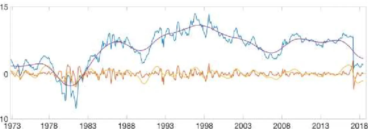
We consider the original time series of the term spread, calculated as the difference between a long and short term governmental rates, and three of its frequency components (high frequency, business cycle frequency and low frequency) as equity risk premium predictors. As explained in section 2.2, the method used to extract these frequency components is the Maximum Overlap Discrete Wavelet Transform Multiresolution Analysis (MODWT MRA), using J=5 level of details. The next set of figures 2-9 illustrate, for each of the eight countries under analysis, the dynamics of the original term spread time series as well as for its three frequencies under analysis. The blue line represents the original time series of the term spread, the orange line denotes the high frequency
component of the term spread, the yellow line represents the business cycle frequency and the purple line reflects the low frequency of the term spread.
Germany
France
Japan
Figure 2: Time series of the term spread and of its different components for Germany
United States of America
United Kingdom
Canada
Figure 5: Time series of the term spread and of its different components for U.S.A
Figure 6: Time series of the term spread and of its different components for U.K
South Africa
Australia
Figure 8: Time series of the term spread and of its different components for South Africa
3.2 In-Sample Forecasting
Following Faria and Verona (2018), let 𝐸𝑅𝑃𝑖,𝑡 represent the equity risk
premium of the country i in month t. For each predictor 𝑥𝑖,𝑡, the predictive
regression is:
𝐸𝑅𝑃𝑖,𝑡:𝑡+ℎ = 𝛼 + 𝛽𝑥𝑖,𝑡+ 𝜀𝑖,𝑡:𝑡+ℎ ∀𝑡 = 1, … , 𝑇 − ℎ (13)
where h represents the forecasting horizon and 𝐸𝑅𝑃𝑖,𝑡:𝑡+ℎ is also given by:
𝐸𝑅𝑃𝑖,𝑡:𝑡+ℎ = 𝐸𝑅𝑃𝑖,𝑡+1+ ⋯ + 𝐸𝑅𝑃𝑖,𝑡+ℎ
ℎ (14)
In the In-Sample predictability analysis we estimate the predictive regression (13), throughout ordinary least squares (OLS), to obtain the 𝛽’s and test their significance. Nevertheless, there are few constraints related to Stambaugh (1999) bias and Campbell and Yogo (2006) in the predictive regression (13). In order to avoid this bias, it was used a heteroscedasticity and autocorrelation-robust t-statistic and a wild bootstrapped p-value was calculated to test the null hypothesis 𝐻0: 𝛽 = 0 against the hypothesis 𝐻1 = 𝛽 > 0 in the predictive
regression (13). Additionally, each predictor variable was standardized to have a standard deviation of one.
Therefore, 546 observations exist for one-month ahead (h=1), 544 observations for three months ahead or one quarter forecasting horizon (h=3), 541 observations for six months ahead or one semester ahead (h=6), 535 observations for one year ahead (h=12) and 523 observations for two years ahead (h=24).
In the next subsections are provided the results of each country for the in-sample analysis for each country.
3.2.1 Results
The following tables report, for each forecasting horizon and each country, the 𝛽 estimates of the predictive model by OLS and the resultant 𝑅2 statistics (given
in percentages). Brackets below the 𝛽 coefficients represent the heteroscedasticity and autocorrelation robust t-statistic for 𝐻0: 𝛽 = 0 against
𝐻1 = 𝛽 > 0 . Moreover, *** denote a significance level of 1%, ** denote a significance level of 5% and * denotes a significance level of 10%, according to bootstrapped p-values. The sample period starts in March 1973 and ends in August 2018.
3.2.1.1 – Germany
Table 2: In-Sample predictive regression results for Germany
The original time series, the business cycle frequency and the low frequency of the term spread, have predictability power of the equity risk premium in all forecasting horizons, although the levels of significance at which the predictors are significant, are decreasing as the forecasting horizon increases. When it comes to the coefficient of determination (𝑅2) we can see that they are rather small, although they increase as the forecasting horizon increases. This is in line with the literature.
Predictor h = 1 h = 3 h = 6 h = 12 h = 24 𝛽̂ 𝑅2 𝛽̂ 𝑅2 𝛽̂ 𝑅2 𝛽̂ 𝑅2 𝛽̂ 𝑅2 𝑇𝑀𝑆𝑇𝑆 0,46 0,78 0,43 1,89 0,42 3,27 0,39 5,67 0,25 4,97 [2,27]*** [2,51]*** [2,56]** [2,47]** [1,87]* 𝑇𝑀𝑆𝐻𝐹 -0,06 0,01 -0,20 0,39 -0,10 0,19 0,02 0,02 0,01 0,02 [-0,25] [-1,07] [-0,65] [0,22] [0,31] 𝑇𝑀𝑆𝐵𝐶𝐹 0,48 0,86 0,47 2,24 0,43 3,54 0,38 5,25 0,24 4,42 [2,12]** [2,45]** [2,37]** [2,26]** [1,84]* 𝑇𝑀𝑆𝐿𝐹 0,43 0,70 0,45 2,02 0,41 3,25 0,37 5,08 0,24 4,59 [2,23]** [2,63]** [2,64]** [2,34]** [1,70]*
3.2.1.2 – France
Table 3: In-Sample predictive regression results for France
It is possible to verify the existence of In-Sample predictability power for France of the original time series, the business cycle component and the smooth component, however it is decreasing as the forecasting horizon increases. Again, the coefficient of determination increases as the forecasting horizon increases.
3.2.1.3 – Japan
Table 4: In-Sample predictive regression results for Japan
For Japan there is no evidence of in-sample predictability power of the equity risk premium from the term spread or any of its frequencies (exception is the low frequency at one-month horizon).
Predictor h = 1 h = 3 h = 6 h = 12 h = 24 𝛽̂ 𝑅2 𝛽̂ 𝑅2 𝛽̂ 𝑅2 𝛽̂ 𝑅2 𝛽̂ 𝑅2 𝑇𝑀𝑆𝑇𝑆 0,54 0,87 0,58 2,77 0,55 4,40 0,48 6,47 0,36 7,82 [1,96]** [2,30]** [2,11]** [2,03]* [2,30]* 𝑇𝑀𝑆𝐻𝐹 -0,22 0,14 -0,07 0,04 -0,07 0,08 -0,01 0,00 -0,03 0,04 [-0,75] [-0,29] [-0,43] [-0,10] [-0,42] 𝑇𝑀𝑆𝐵𝐶𝐹 0,76 1,68 0,66 3,60 0,55 4,34 0,33 3,02 0,15 1,42 [2,71]*** [2,65]** [2,04]** [1,48] [0,93] 𝑇𝑀𝑆𝐿𝐹 0,42 0,51 0,47 1,81 0,51 3,75 0,53 7,71 0,47 13,27 [1,68]* [2,15]** [2,33]** [2,35]** [2,55]** Predictor h = 1 h = 3 h = 6 h = 12 h = 24 𝛽̂ 𝑅2 𝛽̂ 𝑅2 𝛽̂ 𝑅2 𝛽̂ 𝑅2 𝛽̂ 𝑅2 𝑇𝑀𝑆𝑇𝑆 -0,01 0,00 0,13 0,16 0,21 0,65 0,19 1,06 0,25 3,37 [-0,03] [0,64] [0,99] [0,97] [1,48] 𝑇𝑀𝑆𝐻𝐹 -0,83 2,40 -0,36 1,14 -0,08 0,11 -0,11 0,37 -0,01 0,00 [-2,72] [-2,06] [-0,64] [-1,51] [-0,21] 𝑇𝑀𝑆𝐵𝐶𝐹 0,01 0,00 -0,05 0,02 -0,11 0,19 -0,11 0,36 -0,10 0,66 [0,06] [-0,25] [-0,47] [-0,45] [-0,74] 𝑇𝑀𝑆𝐿𝐹 0,29 0,29 0,30 0,80 0,30 1,40 0,30 2,58 0,35 5,97 [1,40]* [1,46] [1,41] [1,45] [1,80]
3.2.1.4 – United States of America
Table 5: In-Sample predictive regression results for U.S.
This table demonstrates one more country where it is possible to observe the significance of the predictors, yet in a different way. For the United States of America, we can observe the presence of significant predictors mostly for forecasting horizons of one month. The original times and the high frequency component are significant at 1% level, whereas the business cycle frequency and the low frequency component, though significant, are relevant at minor levels of significance. Again, the coefficients of determination are increasing as the forecasting horizon increases.
3.2.1.5 – United Kingdom
Table 6: In-Sample predictive regression results for U.K
The empirical evidence of in-sample predictability in United Kingdom has a similar with that of Japan. There are almost no significant predictors with the
Predictor h = 1 h = 3 h = 6 h = 12 h = 24 𝛽̂ 𝑅2 𝛽̂ 𝑅2 𝛽̂ 𝑅2 𝛽̂ 𝑅2 𝛽̂ 𝑅2 𝑇𝑀𝑆𝑇𝑆 0,48 1,11 0,35 1,75 0,26 1,78 0,25 3,39 0,19 4,46 [2,36]*** [1,85]* [1,50] [1,64] [1,75] 𝑇𝑀𝑆𝐻𝐹 0,55 1,49 0,18 0,47 -0,04 0,05 0,00 0,00 -0,02 0,04 [2,60]*** [1,05] [-0,39] [-0,01] [-0,63] 𝑇𝑀𝑆𝐵𝐶𝐹 0,40 0,78 0,35 1,77 0,27 1,96 0,19 1,86 0,10 1,16 [1,86]** [1,76]* [1,43] [1,25] [0,75] 𝑇𝑀𝑆𝐿𝐹 0,25 0,30 0,25 0,91 0,26 1,85 0,28 4,18 0,25 7,26 [1,33] [1,53]* [1,57] [1,75]* [2,41]* Predictor h = 1 h = 3 h = 6 h = 12 h = 24 𝛽̂ 𝑅2 𝛽̂ 𝑅2 𝛽̂ 𝑅2 𝛽̂ 𝑅2 𝛽̂ 𝑅2 𝑇𝑀𝑆𝑇𝑆 0,03 0,00 0,12 0,15 0,17 0,55 0,24 2,42 0,21 5,33 [0,10] [0,48] [0,81] [1,55] [1,83]* 𝑇𝑀𝑆𝐻𝐹 -0,20 0,14 0,07 0,05 0,07 0,10 0,19 1,42 0,03 0,08 [-0,73] [0,24] [0,33] [1,29]* [0,53] 𝑇𝑀𝑆𝐵𝐶𝐹 0,12 0,05 0,18 0,32 0,25 1,20 0,28 3,35 0,13 2,03 [0,42] [0,74] [1,15] [1,32] [1,27] 𝑇𝑀𝑆𝐿𝐹 0,03 0,00 0,05 0,03 0,07 0,11 0,12 0,61 0,21 5,49 [0,12] [0,22] [0,36] [0,78] [1,85]*
considering the significance of these predictors, they are all significant only at 10%. In addition, the 𝑅2are increasing as the forecasting horizon increases, but they are slightly lower than the 𝑅2 verified in the other countries.
3.2.1.6 – Canada
Table 7: In-Sample predictive regression results for Canada
For Canada, it is observable that the two significant predictors are the original time series and the business cycle frequency. Furthermore, we can see the significance of lower frequency, for forecasting horizons of 12 and 24 months, of 10% and 5% respectively. The coefficient of determination does not always increase as the forecasting horizon increases, although we can verify that it is rather small when the predictor is not significant.
3.2.1.7 – South Africa
Table 8: In-Sample predictive regression results for South Africa
Predictor h = 1 h = 3 h = 6 h = 12 h = 24 𝛽̂ 𝑅2 𝛽̂ 𝑅2 𝛽̂ 𝑅2 𝛽̂ 𝑅2 𝛽̂ 𝑅2 𝑇𝑀𝑆𝑇𝑆 0,35 0,63 0,30 1,25 0,33 2,81 0,34 5,88 0,23 7,23 [1,82]** [1,73]* [1,98]* [2,18]* [2,93]** 𝑇𝑀𝑆𝐻𝐹 0,05 0,01 -0,15 0,31 -0,08 0,17 0,04 0,10 -0,01 0,03 [0,27] [-0,89] [-0,74] [0,47] [-0,33] 𝑇𝑀𝑆𝐵𝐶𝐹 0,45 1,03 0,46 2,86 0,46 5,34 0,33 5,76 0,12 2,13 [2,14]** [2,42]** [2,55]** [2,13]* [1,28] 𝑇𝑀𝑆𝐿𝐹 0,22 0,25 0,23 0,75 0,25 1,58 0,28 4,11 0,28 10,77 [1,15] [1,41] [1,50] [1,79]* [2,76]** Predictor h = 1 h = 3 h = 6 h = 12 h = 24 𝛽̂ 𝑅2 𝛽̂ 𝑅2 𝛽̂ 𝑅2 𝛽̂ 𝑅2 𝛽̂ 𝑅2 𝑇𝑀𝑆𝑇𝑆 0,07 0,01 0,06 0,02 0,05 0,04 0,06 0,12 0,01 0,00 [0,20] [0,20] [0,20] [0,24] [0,04] 𝑇𝑀𝑆𝐻𝐹 0,29 0,20 0,18 0,23 0,04 0,02 0,12 0,47 0,01 0,01 [0,94] [0,83] [0,20] [1,13]* [0,16] 𝑇𝑀𝑆𝐵𝐶𝐹 0,15 0,05 0,21 0,30 0,27 0,96 0,30 2,51 0,19 2,13 [0,61] [1,05] [1,31] [1,41] [1,31] 𝑇𝑀𝑆𝐿𝐹 -0,02 0,00 -0,03 0,00 -0,02 0,00 -0,03 0,02 -0,04 0,10 [-0,06] [-0,08] [-0,06] [-0,10] [-0,20]
The only country belonging to the African continent seems to have similar results to Japan and United Kingdom. There is extremely little evidence of in-sample predictability power of the term spread and its frequency components over the equity risk premium.
3.2.1.8 – Australia
Table 9: In-Sample predictive regression results for Australia
Obtained results for Australia are similar to those found in the group of Japan, United Kingdom and South Africa. There is no evidence supporting the existence of in-sample predictability power for none of the predictors and for none of the forecasting horizons.
Overall, this set of empirical results support the existence of a subsample of countries (Germany, France, United States of America and Canada) where it is found statistically significant in-sample predictability of the equity risk premium, using both the original time series of the term spread and of its frequencies and for different horizons, while for other of countries (Japan, United Kingdom, South Africa and Australia) there is no evidence of in-sample predictability. Predictor h = 1 h = 3 h = 6 h = 12 h = 24 𝛽̂ 𝑅2 𝛽̂ 𝑅2 𝛽̂ 𝑅2 𝛽̂ 𝑅2 𝛽̂ 𝑅2 𝑇𝑀𝑆𝑇𝑆 0,34 0,39 0,32 0,97 0,23 0,96 0,09 0,29 -0,01 0,01 [0,87] [0,85] [0,83] [0,52] [-0,14] 𝑇𝑀𝑆𝐻𝐹 0,28 0,26 0,25 0,58 0,12 0,25 0,03 0,05 0,00 0,00 [0,52] [0,63] [0,49] [0,37] [0,02] 𝑇𝑀𝑆𝐵𝐶𝐹 0,36 0,42 0,35 1,14 0,25 1,16 0,04 0,06 -0,11 1,24 [0,89] [0,92] [0,86] [0,24] [-1,33] 𝑇𝑀𝑆𝐿𝐹 0,10 0,03 0,10 0,09 0,11 0,21 0,10 0,35 0,08 0,57 [0,37] [0,38] [0,48] [0,52] [0,74]
3.3 Out-Of-Sample Forecasting
In recent decades, out-of-Sample predictability has become a relevant method of forecasting financial variables. This method is particularly relevant in financial and economic terms because is closed to real-world prediction once it uses information available until the moment of predictability to predict.
We start with an in-sample period from March 1973 until December 1989 in order to make the first OOS estimate. Afterwards, the sample increases by one observation, as the OOS forecast is generated using a sequence of expanding windows and the process runs until the end of the sample.
The three OOS periods considered are: the full OOS period that starts in January 1990 and ends in August 2018. The next two periods are a division of this full period and run from January 1990 to December 2006 and January 1997 till August 2018.
Following Faria and Verona (2018), the equation that represents the h-step-ahead forecast of equity risk premium is given by:
𝑟̂𝑡:𝑡+ℎ = 𝛼̂𝑡+ 𝛽̂𝑡𝑥𝑡 (15)
where 𝑟̂𝑡:𝑡+ℎ denotes the h-step-ahead forecast equity risk premium of the
month t until month t+h, and 𝛼̂𝑡 and 𝛽̂𝑡 represent the OLS estimators of and
respectively of month t, using observations from the beginning of the dataset until month t.
As in Faria and Verona (2018), the evaluation of OOS forecasting performance is done throughout Campbell and Thomson (2007) 𝑅𝑂𝑆2 statistic. As it is standard
in the literature, the historical mean (HM) forecast 𝑟̅𝑡, which represents the
The 𝑅𝑂𝑆2 statistic is calculated in the following way:
𝑅𝑂𝑆2 = 100 (1 −𝑀𝑆𝐹𝐸𝑃𝑅𝐸𝐷
𝑀𝑆𝐹𝐸𝐻𝑀 ) (16)
where 𝑀𝑆𝐹𝐸𝑃𝑅𝐸𝐷 is the mean squared forecast error of the predictive model,
while 𝑀𝑆𝐹𝐸𝐻𝑀 represents the mean squared forecast error of the historical mean
given by: 𝑀𝑆𝐹𝐸𝑃𝑅𝐸𝐷 = ∑ (𝑟𝑡:𝑡+ℎ− 𝑟̂𝑡:𝑡+ℎ)2 𝑇−ℎ 𝑡=𝑡0 (17) 𝑀𝑆𝐹𝐸𝐻𝑀 = ∑ (𝑟𝑡:𝑡+ℎ− 𝑟̅𝑡:)2 𝑇−ℎ 𝑡=𝑡0 (18)
where 𝑟̂𝑡:𝑡+ℎ represents the excess return forecast from the model with each of
the alternative predictors.
The 𝑅𝑂𝑆2 therefore measure the reduction in the mean squared forecast error
from the usage of the predictive model relative to the historical mean.
The predictive model outperforms (underperforms) historical average in terms of MSFE if the 𝑅𝑂𝑆2 is positive (negative).
Similarly to Rapach, Ringgenberg, and Zhou (2016) and Faria and Verona (2018) the statistical significance of the results is analyzed using the Clark and West (2007) statistic. Here, the null hypothesis is verified when the MSFE of the historical mean is smaller or equal to the MSFE of the predictive model and the alternative hypothesis is validated when the MSFE of the historical mean is greater than the MSFE of the predictive model (𝐻0: 𝑅𝑂𝑆2 ≤ 0 against 𝐻𝐴: 𝑅𝑂𝑆2 > 0).
3.3.1 Analysis of Results
The following tables present 𝑅𝑂𝑆2 (in percentages) for the equity risk premium
forecast of the full OOS period (1990:01 – 2018:08) for the same forecasting horizons considered in the in-sample analysis, of each predictor. Moreover, asterisks denote the significance of OOS MSFE-adjusted statistic of Clark and West (2007). *** represent significance at 1%, ** denote significance at 5% and * symbolizes significance at 10%.
3.3.1.1 Germany
Table 10: Out-of-Sample R-squares for Germany
By analyzing the results, we can state that the original time series (𝑇𝑀𝑆𝑇𝑆) and the low frequency component ( 𝑇𝑀𝑆𝐿𝐹 ) of the term spread
outperform the historical mean benchmark (positive and statistically significant 𝑅𝑂𝑆2
)
for almost all forecast horizons. On the other hand, the high frequency (𝑇𝑀𝑆𝐻𝐹) and the business cycle (𝑇𝑀𝑆𝐵𝐶𝐹)
components are poor OOS predictors, as they have a negative or non-significant 𝑅𝑂𝑆2 (excepting for forecasting horizonsof 12 and 24 months in the business cycle frequency).
Predictor 𝑅𝑂𝑆 2 h = 1 h = 3 h = 6 h = 12 h =24 𝑇𝑀𝑆𝑇𝑆 0,76** 1,74** 3,09** 5,54** 4,87* 𝑇𝑀𝑆𝐻𝐹 -0,18 -0,63 -0,70 -0,35 -0,07 𝑇𝑀𝑆𝐵𝐶𝐹 0,02 0,06 0,48 2,25* 3,00* 𝑇𝑀𝑆𝐿𝐹 0,96** 2,24** 3,52* 4,87** 3,00
3.3.1.2 France
Table 11: Out-of-Sample R-squares for France
France has a very similar behavior to Germany but with smaller 𝑅𝑂𝑆2 . Again,
the original time series appears to be a good OOS predictor with positive 𝑅𝑂𝑆2 and
significant for forecasting horizons starting at 3 months. However, the low frequency of the term spread loses value for historical mean benchmark for forecasting horizons superior to twelve months. Nevertheless, 𝑇𝑀𝑆𝐿𝐹 beats the
HM benchmark in forecasting horizons up to 6 months. The high and business cycle frequency of the term spread reveal to be a poor OOS predictor of the term spread, which is surprising given the statistical significance of the business cycle in in-sample analysis.
3.3.1.3 Japan
Table 12: Out-of-Sample R-squares for results for Japan
When it comes to the OOS analysis for Japan, all the predictors appear to have no predictive power in all forecasting horizons. The 𝑅𝑂𝑆2 are all negative, which
Predictor 𝑅𝑂𝑆 2 h = 1 h = 3 h = 6 h = 12 h =24 𝑇𝑀𝑆𝑇𝑆 0,16 1,25** 2,59** 3,48** 6,85** 𝑇𝑀𝑆𝐻𝐹 0,19 0,12 0,04 -0,56 -2,17 𝑇𝑀𝑆𝐵𝐶𝐹 -0,82 -0,88 -0,64 -0,11 -1,63 𝑇𝑀𝑆𝐿𝐹 0,77* 1,41** 1,37** -2,78 -8,16 Predictor 𝑅𝑂𝑆 2 h = 1 h = 3 h = 6 h = 12 h =24 𝑇𝑀𝑆𝑇𝑆 -2,33 -3,08 -4,03 -10,04 -13,32 𝑇𝑀𝑆𝐻𝐹 -2,14 -1,38 -0,93 -2,31 -7,62 𝑇𝑀𝑆𝐵𝐶𝐹 -1,04 -3,51 -5,63 -9,82 -8,71 𝑇𝑀𝑆𝐿𝐹 -0,83 -3,28 -6,93 -12,87 -23,23
3.3.1.4 United States of America
Table 13: Out-of-Sample R-squares for for U.S
The United States of America is the first country where we can observe clear evidence of the predictability power of the low frequency component of the term spread on all forecasting horizons.
Here, the 𝑇𝑀𝑆𝐿𝐹 has a positive and statically significant 𝑅𝑂𝑆2 for all forecasting
horizons, meaning that the smooth component outperforms the historical mean benchmark. This result matches the results obtained by Faria and Verona (2018) who found that “the low frequency component of the term spread, when extracted using wavelet filtering methods, has remarkably robust empirical equity premium OOS forecasting power.”
3.3.1.5 United Kingdom
Table 14: Out-of-Sample R-squares for U.K
Predictor 𝑅𝑂𝑆 2 h = 1 h = 3 h = 6 h = 12 h =24 𝑇𝑀𝑆𝑇𝑆 -0,89 -1,64 -1,60 0,22 4,32** 𝑇𝑀𝑆𝐻𝐹 -0,74 -0,72 -0,26 -0,45 0,61 𝑇𝑀𝑆𝐵𝐶𝐹 -2,49 -7,24 -10,21 -7,34 1,07 𝑇𝑀𝑆𝐿𝐹 0,31* 1,01** 2,26** 5,74*** 11,21*** Predictor 𝑅𝑂𝑆 2 h = 1 h = 3 h = 6 h = 12 h =24 𝑇𝑀𝑆𝑇𝑆 -0,33 -0,36 -0,07 0,42 -9,89 𝑇𝑀𝑆𝐻𝐹 0,40 -0,65 -1,02 -4,59 -13,51 𝑇𝑀𝑆𝐵𝐶𝐹 -0,16 -0,56 -1,46 -5,11 -15,51 𝑇𝑀𝑆𝐿𝐹 -0,24 -0,48 -0,40 -0,43 -7,20