Development of an univariate method for
predicting traffic behaviour in wireless
networks through statistical models
Jorge E Salamanca Céspedes #1, Yaqueline G. Rodríguez #2, Danilo A López Sarmiento #3
# 1
FullTime Professor at Universidad Distrital Francisco José de Caldas, Faculty of Engineering, Bogotá (Colombia-South America)
Full Time Professor at Universidad Distrital Francisco José de Caldas, Faculty of Technology, Bogotá (Colombia-South America)
Full Time Professor at Universidad Distrital Francisco José de Caldas, Faculty of Engineering, Bogotá (Colombia-South America)
Abstract— Today has shown that modern traffic in data networks is highly correlated, making it necessary to select this kind of models that capture autocorrelation characteristics governing data flows surrounding on the network [1].
Being able to perform accurate forecasting of traffic on communication networks, this has great importance at present, since it influences decisions as important such as network sizing and predestination.
The main purpose in this paper is to put into context the reader about the importance of statistical models of time series, it enable for estimating future traffic forecasts in modern communications networks, and becomes an essential tool for traffic prediction, This prediction according to the individual needs of each network are listed in estimates with long range dependence (LDR) and short-range dependence (SDR), each one providing a specific control, appropriate and efficient integrated at different levels of the network functional hierarchy [2].
But for the traffic forecasts in the modern communication networks must define the type of network to study and time series model that fits the same, which is why you should first select the type of network. For this case study, is a Wi-Fi network as the traffic behavior requires the development of a time series model with advanced statistics, that allows an integrated observing network and thus provide a tool to facilitate the monitoring and management of the same. According to this the type of time series model to use for this case are the ARIMA time series.
Keyword- Autocorrelation, ARIMA, correlation, stochastic traffic model, time series, WiFi network.
I. INTRODUCTION
The importance of predicting the flow behavior in wireless networks is that from these models is possible inter alia known beforehand the characteristics required for optimal data transfer between a sender and a receiver. This is why traffic dimensioning has become an extensive area of research in which the aim is to develop patterns that predict the impact of the load imposed by different applications on network resources [3].
These new features in capabilities and claims, allow detect inconsistencies between traditional schemes, based on uncorrelated traffic and observed measurements in new information flow especially in regard to correlation structures that are present along different time scales [4].
Demonstrating that the current traffic in wireless communication networks is too complex to be modeled by uncorrelated events, it becomes necessary to create statistical models allowing the prediction of flow behavior in new communications networks, and in our specific case on WI-FI networks, that is one of the most used technologies into users at last mile technologies level.
For this reason, it has been necessary develop additional traffic models capable of representing these correlations taking into account the data characteristics that really surround networking structure, especially the correlations between inter-arrival times, completely absent in the uncorrelated models.
Current traffic in communication networks is determined largely by development and new technologies use, such as wireless networks allow greater access to multiple users, something that influences forecast traffic [5].
Currently, communication network technology development, is booming, so it has ample space to make significant contributions through research activities at the knowledge frontier.
II. BACKGROUND
In a significant percentage, currently on track to study traffic engineering is governed by methods that are not consistent with transferred data, for this reason it is important explore other tools to improve substantially the prediction in future flows. Models based on time series focus on make univariate forecasting traffic, ie concentrate its forecast around time variable [3]. Such drivers can become beneficial for coverage planning, resource reservation, network monitoring, anomaly detection, and production simulation models more accurate than those based on Markov chains, for example, to the extent that can predict traffic on a given time scale [8].
For this reason time series studying aim for this specific case is to develop statistical models to make future forecasting data of a random variable that changes over time or respect to other indices are considered influence behavior of the same.
Time series use is extremely important as it gives the possibility to find methods that minimize error prediction [9] thus increasing the reliability of forecasting data and therefore reducing the uncertainty future can cause, hence, this statistical tool is a method applicable in planning and knowledge areas where knowing predictions of future values contribute to reduce risk in decision-making and provide important criteria in implementing future policies [4].
Specifically time series is an observations set for a variable measured on successive points or periods in time, and if the data or historical information is restricted to past variable values [10], forecasting procedure is called time series method, currently there are several techniques for analyzing time series, whose main objective is discover behavior on historical data (past variable values and/or past prediction mistakes) in order to future extrapolation and provide good predictions in future series values.
Time interval between the present and the time at which the event of interest will occur is called time forecast or leading time and gives need rise to meet event forecast, in order to plan and implement actions to counter or monitor the effects that such an event occur [11]. The length of this time interval gives planning rise, if don´t exist or is very small, it would be facing specific situations should be resolved through immediate action, but not planned.
Consequently, when forecast time is appropriate and interest outcome event is determined by identifiable factors, planning makes sense and knowledge forecast event allows decisions on actions to execute or control for final results are consistent with general policy company.
It is important to note that there are factors that influence forecast quality. These can be internal or controllable and external or uncontrollable and planning success will depend on them. However, note that external factors can only be predicted and taken into account when making decisions, while the inner well predicted chords can be controlled by the policy company decisions and with external factors acting on them. ARIMA time series was implemented in future estimates development as it is a statistical time series whose primary objective is the statistical analysis that explains behavior random variable, for this traffic case WI-FI networks regarding a variable which in our case is time.
III.METHODOLOGY FOR OBTAINING THE MODEL
This section relates methodology for developing univariate model, firstly refers to the generation and processing that data had suffer to construct series, subsequent, modeling ARIMA for future dynamics traffic from taking 80% of the original frame sequence, finally validates the proposed effectiveness contrast future dynamic found with ARIMA, compared actual realized the remaining 20% of the original flow.
A. Data collection and series time construction.
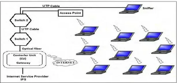
To capture data was used Wireshark network analyzer as it is a very useful tool for monitoring and managing a data network, it´s free software to analyze a wireless data network (Wi-Fi).
Fig. 1. WI-FI architecture network, which arrest was made
In analysis and data processing, a classification is initially made of the protocols by reference those that represent a larger percentage in the catch made for each day, the above in order to remove the least significant protocols, but this classification a drawback at analyze traffic time, many protocols in application layer, which are currently considered as the most important in prediction time for contemporary traffic network should be considered less significant. For these reasons it is necessary to classify all the protocols found in the traffic capture, for identification was used TCP / IP model. Last in order to identify standards belonging to the application layer, and discriminating. Table I, list 15 application layer protocol found in the catch.
TABLE I Application protocols
Application Protocols
ID Description ID Description
1 DHCP 9 SMB_NETLOGON
2 DHCPv6 10 SNMP
3 DNS 11 SSDP
4 HTTP 12 SSLv2
5 HTTP/XML 13 SSLv3
6 LLMNR 14 TLSv1
7 MDNS 15 NTP
8 SMB
Having identified application protocols, it is necessary to establish a delta time, decided for data discretization in the time series a two (2) minutes delta time reorganizing captured information, for this time period for which the information contained in it is transformed into a single data traffic.
But take this time to the discretization of data presents a problem as it is necessary to handle a considerable amount of data, above and taking as selection criteria, large capacity and data management, best time in processing generate data and functionality enabling robust queries whether simple or complex , decides work with MYSQL, addition because programing in PHP and facilitates author management and control.
Taking two minutes periods, in such variable occurs more than one protocol during the same time interval, so the solution was seen assign a code for each possible combination, this numeric code identifies up to 136 and is performed programmatically in Excel. These 15 selected protocols generated approximately 80% in all traffic and their percentages are significant.
TABLE III
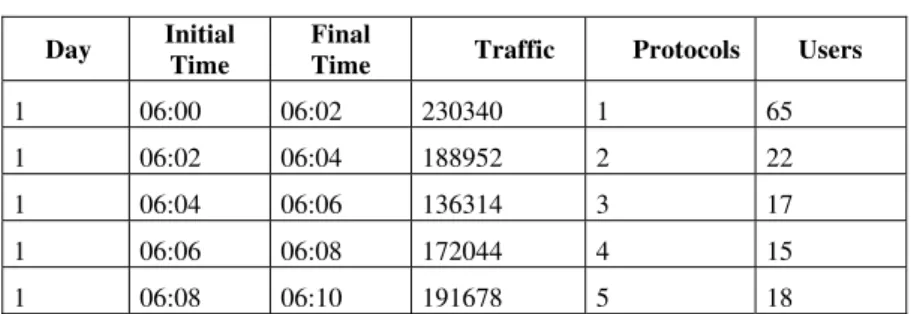
Original time series fragment for day
Day Initial
Time
Final
Time Traffic Protocols Users
1 06:00 06:02 230340 1 65
1 06:02 06:04 188952 2 22
1 06:04 06:06 136314 3 17
1 06:06 06:08 172044 4 15
1 06:08 06:10 191678 5 18
First column corresponds to the number of day which traffic catching. Second column corresponds to the initial time variable, which corresponds to the time which traffic data obtained, this value was obtained from programming in PHP. Third column corresponds to the final time variable. Fourth column corresponds to the traffic variable (dependent variable or explained) measured in bytes per minute, this measure can also be performed in packets per minute, but is usually used bps or kbps or Mbps. Fifth column corresponds to the assigned number for protocol combination originated for this same interval (see Table II).
B. Applied Statistical Modeling obtained data with Time Series ARIMA and VAR.
As previously mentioned, it was necessary assign a numerical protocols code combinations presents at each time deltas (two minutes traces), whereby it becomes necessary to verify protocol and users variables significant have, correlation matrix for Traffic, user and protocol variables on day 1 is related in Table III.
TABLE IIIII
Correlation matrix for traffic protocol and user variables
Day1 Traf1 Prot1 User1
Traf1 1.000 0.412 0.5618
Prot1 0.412 1.000 0.016
User1 0.561 0.016 1.000
For the last could be see first that Traffic variable correlates by 42%, with Protocol variable which although not a high ratio could be consider as significant. On the other hand Traffic variable correlates with User variable by 56%, ratio could be estimated as significant.
After review significance degree for each of the variables in forecasting traffic variable, these values were used for series traffic modeling by ARIMA method; for this worked series in logarithms [10], it was found that so softened its variance and was easier to model them, under the parsimony principle. The model was developed through Rats Software Version 7.2 for series case.
C. Series ARIMA procedure
Following describes executed steps for the series. Initially we proceeded to perform series, protocol and users, graphical analysis, then move to the unit root tests, in order to know whether the series are stationary or not. Then carried out the identification process, estimation and diagnosis for possible models for each series. The procedure is described in Fig. 2.
IV.DEVELOPED MODEL WITH ARIMA AND RESULTS
yes
not
Fig. 2. Series ARIMA and VAR procedure
Fig. 3. Original time series traffic for day one
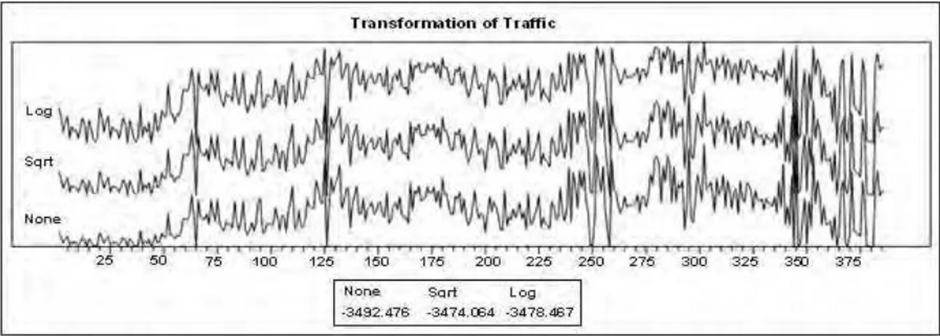
Fig. 4 shows the original series and square root transformations and log in it shows that although the series is scaled to different changes their behavior not, so apparently its variance is constant.
Data for a series time
Step 1: Series graph
Step 3: Transformation and
differentiation Step 2:
Dickey-Fuller test
Step 4: Model identification
Step 5: Model estimation
Fig. 4. Time series transforms
Fig. 5 shows the original series, the series with log transformed and once differentiated transformed series where apparently unique in having a constant average is the differentiated and transformed once.
Fig 5. Transformed time series and difference for day one
In order to estimate the possible data generating processes underlying the aforementioned series and find in them the possible existence of stochastic trends linked, they became unit root tests. These tests were performed using statistical Dickey-Fuller for the series in logarithms and their differences. This formal test helps determine if a system has constant average, ie if it is stationary. The results reported in Table IV.
TABLE IVV Dickey-Fuller test result
Dickey-Fuller test for original time series. X
Dickey-Fuller test for time series transformed with log. LX
Dickey-Fuller test for time series transformed and differentiate once a time. DLX
DICKEY-FULLER TEST FOR X WITH 6 LAGS: -0.5955 *
AUGMENTED DICKEY-FULLER TEST FOR LX WITH 7 LAGS: 0.2401 *
AUGMENTED DICKEY-FULLER TEST FOR DLX WITH 6 LAGS: -13.6449 *
* AT LEVEL 0.05 THE TABULATED CRITICAL VALUE: -1.9404 *
As the critical value must be greater than the statistic, to 5% there is enough statistical evidence to reject the null hypothesis that the time series is not stationary, for the time series transformed and differentiated once DLX.
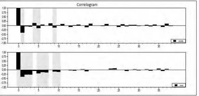
Fig 6. Correlogram for capture samples day. Calculations by the author using the Rats.
In simple autocorrelation function figure could see that non-zero lags are 1, 4.5 and 9.In the partial autocorrelation function graph identifies the lags 1, 2, 3, 5, 6, 7,9 and 10.
With the above estimates the first model with q = 1, 4, 5 and 9 and p = 1, 2, 3, 5, 6, 7, 9 and 10. Whereupon the following results are obtained, reported in Table V, thrown by statistical package Rats.
TABLE V
First ARIMA model result for day one
Variable Coeff Std Error T-Sta Signif
1. AR{1} 0.981207121 0.049938405 -19.64835 0.00000000
2. AR{2} 069231395 0.062921889 -16.99300 0.00000000
3. AR{3} -1.096316084 0.038606421 -28.39725 0.00000000
4. AR{5} -0.194189268 0.071003403 -2.73493 0.00654806
5. AR{6} -0.075180694 0.073798897 -1.01872 0.30901823
6. AR{7} 0.090800597 0.036939514 2.45809 0.01443828
7. AR{9} 0.092143504 0.042677386 2.15907 0.03150480
8. AR{10} 0.061721115 0.043393384 1.42236 0.03150480
9. MA{1} -0.476421240 0.068086135 -6.99733 0.00000000
10. MA{4} -1.038056130 0.051992591 -19.96546 0.00000000
11. MA{5} 0.627163987 0.082162438 7.63322 0.00000000
12. MA{9} 0.022813221 0.069445581 0.32851 0.74272085
In this table we can identify coefficients for the autoregressive lags part that are significant are 1, 2, 3 and 5. And for the moving average is significant lag 1, 4 and 5.According to the data in Table VI, obtains the final model that corresponds to an ARIMA (3.1, (1.5)), the respective equation is:
TABLE VI Rats software result
Variable Coeff Std Error T-Sta Signif
1. AR{1} -0.610617275 0. 050644554 -12.05692 0.00000000
2. AR{2} -0.470306578 0.045279364 -10.38678 0.00000000
3. AR{3} -0.316542511 0.043497563 -7.27725 0.00000000
5 1
3 2
1
0
.
470
0
.
316
116
0
.
17
61
.
0
−−
−−
−+
−
−+
−−
=
t t t t t tt
y
y
y
a
a
a
y
A. Evaluation Model and Self Interpreting Statistics
Initially we present the diagnosis and analysis for univariate and multivariate series respectively and for its evaluation prognosis is 16 hours with the ARIMA and VAR model obtained; finally checks its involvement in the traffic forecast specifically in regard to sizing bandwidth WI-FI links.
Then diagnosis relates model obtained by ARIMA series.
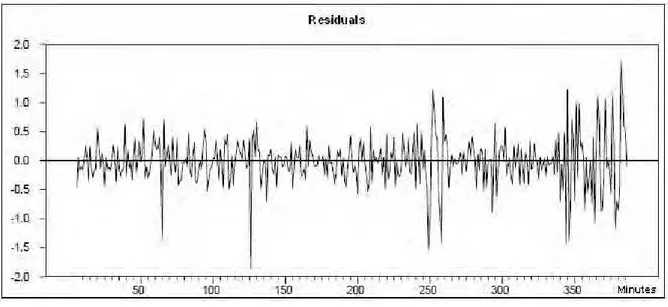
1) Residuals with constant variance. Fig. 7 shows the residuals have no behavior therefore have constant variance.
Fig 7. Waste, ARIMA
2) Residuals with zero average: Table VII shows the summary statistics of the residuals where could be find the proof to confirm whether they have zero average, p-value that yields output 0.504199> 0.05 so the null hypothesis is not rejected, so the residuals have zero average.
TABLE VII
Statistics residuals summary, calculations by the auto using Rats software
Statistics on series R2 Observations 374
Sample means 0.015139 Variance 0.192794
Standard Error 0.439083 of Sample Mean 0.022704
t-Statistic (Mean=0) 0.666772 Signif Level 0.505330
Skewness 0.010190 Signif Level (Sk=0) 0.936138
Kurtosis (excess) 3.412655 Signif Level (Ku=0) 0.000000
Jarque-Bera 181.493296 Signif Level (JB=0) 0.799026
Table VIII shows Jarque-Bera test in which the null hypothesis is that the residuals are normally distributed, the p-value is 0.7990>0.05 so the thesis is not rejected, so the waste if normally distributed.
TABLE VIII
Test result Jaque-Bera (JB). Calculations by Author using the Rats software
Statistics on Series R2 Observations 374
Sample Mean 0.015139 Variance 0.192794
Standard Error 0.439083 of Sample Mean 0.022704
t-Statistic (Mean=0) 0.666772 Signif Level 0.505330
Skewness 0.010190 Signif Level (Sk=0) 0.936138
Kurtosis (excess) 3.412655 Signif Level (Ku=0) 0.000000
Jarque-Bera 181.493296 Signif Level (JB=0) 0.799026
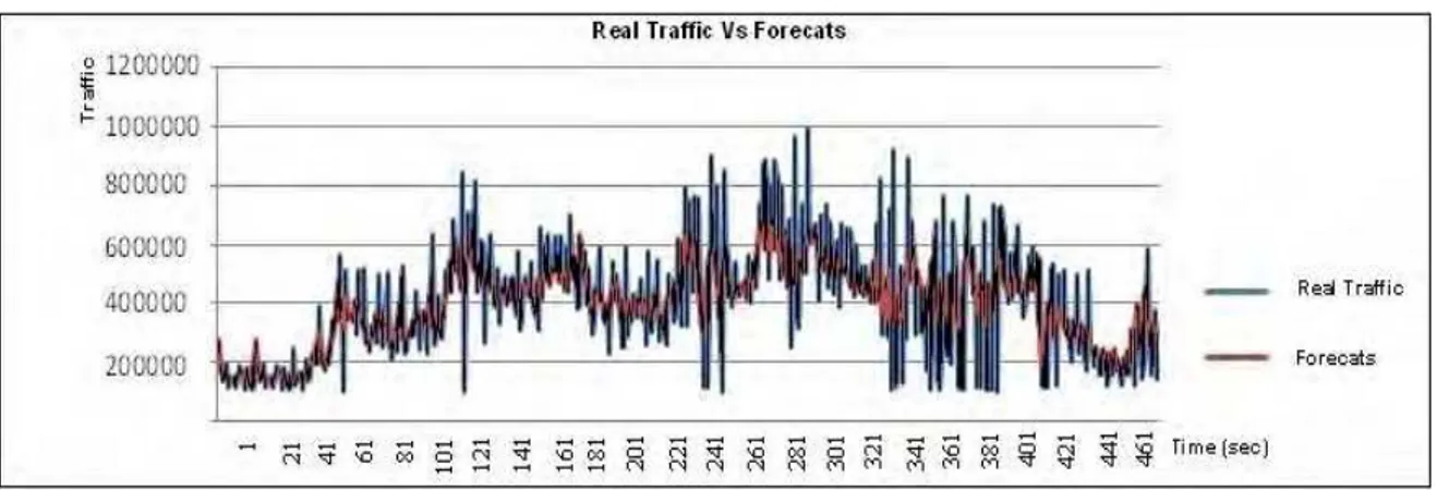
3) Forecast Model.After model diagnosis and see which meets the assumptions will forecast for 16 hours
from 6:00 am to 10:00 pm, for traffic variable is main studied in this work so could make the parallel graph with the original data for each of the series, the results can be seen in Fig. 8.
Fig 8. Real traffic series Vs Forecasts
Could see that the behavior of the series is too similar to the predictions generated by the model into 16 hours so it is concluded that the fit is good for the series, traffic.
V. CONCLUSIONS
ARIMA time series are statistical models which have good approximation for predicting future behaviors when it apply to wireless telecommunications networks, reaching levels of prediction over 90% when estimation times do not exceed hours.
With unchanged statistical model development through ARIMA time series, get a low prediction error, for the specific case of the series explained variable traffic by explanatory metric time, the error rate was 0.4%.
Evaluating the accuracy time estimating traffic series only 80% data was performed by calculating the percentage of the average absolute, deviation mean and variance of the error in predicting 20% of the remaining data, was obtained 4, 87% error. This allows to affirm that there is a level of approximation to the original data quite good.
The forecast made by the ARIMA model for a same dimension time interval daily catch (ie 16 hours) was quite satisfactory as to make the comparison between the original data and the predicted results were very close to original for the series.
REFERENCES
[1] M. Alzate, Modelos de tráfico en análisis y control de redes de comunicaciones, Revista Ingeniería de la Universidad Distrital
Francisco José de Caldas. Bogotá. Vol. 9, No. 1, pp. 63- 87, July 2004.
[2] M. Arino, P. Franses, Forecasting the levels of vector autoregressive log-transformed time series, International Journal of Forecasting.
Amsterdam: Tomo 16, Nº 1, pp. 111, January-March 1999.
[3] G. Bidisha, B. Biswajit, O'M. Margaret, Bayesian time-series model for short-term traffic flow forecasting, Journal of Transportation
Engineering Journal of Transportation Engineering, New York, Tomo 133, Nº 3; pp. 180, March 2007.
[4] A. Casilari, A. Reyes, E. Díaz, F. Sandoval F, Caracterización de tráfico de vídeo y tráfico Internet, Departamento de Tecnología
Electrónica, E.T.S.I Telecomunicación, Universidad de Málaga, Campus de Teatinos, España, 2002.
[5] Y. Chiu, J. Shyu, Applying multivariate time series models to technological product sales forecasting, International Journal of
Technology Management, Tomo 27, Nº 2, Genova, pp. 306, 2004.
[6] E. Correa, Series de tiempo conceptos básicos, Universidad Nacional de Colombia, Facultad de Ciencias, Departamento de
[7] N. Groschwitz, C. George, A time series model of long-term NSFNET backbone traffic, Computer Systems Laboratory, Department of Computer Science and Engineering, University of California, San Diego, August 2003.
[8] A. Dainotti, A. Pescapé, S. Pierluigi, P. Francesco, V. Giorgio, Internet traffic modeling by means of hidden Markov Models,
Computer Networks, Amsterdam: Tomo 52, Nº 14; pp. 2645 – 2662, October 2008.
[9] C. Hernández, Desarrollo de un modelo estadístico que permita estimar pronósticos futuros de tráfico en redes Wimax a través del
modelamiento en series de tiempo, Tesis de Maestría Universidad Distrital, 2007.
[10] C. Hernández, An ARIMA model for forecasting Wi-Fi data network traffic values, Revista Ingeniería e Investigación, ISSN:
0120-5609, Universidad Nacional de Colombia. Volumen 29, Número 2, pp. 65-69, August 2009.
[11] W. E. Leland, M. S. Taqqu, W. Willinger, D. W. Wilson, On the self-similar nature of Ethernet traffic, IEEE/ACM Transaction