www.biogeosciences.net/13/6067/2016/ doi:10.5194/bg-13-6067-2016
© Author(s) 2016. CC Attribution 3.0 License.
BVOC emissions from English oak (
Quercus robur
) and European
beech (
Fagus sylvatica
) along a latitudinal gradient
Ylva van Meeningen1, Guy Schurgers2, Riikka Rinnan3, and Thomas Holst1,3
1Department of Physical Geography and Ecosystem Science, Lund University, Sölvegatan 12, 223 62 Lund, Sweden 2Department of Geosciences and Natural Resource Management, University of Copenhagen, Øster Voldgade 10, 1350 Copenhagen K, Denmark
3Terrestrial Ecology Section, Department of Biology, University of Copenhagen, Universitetsparken 15, 2100 Copenhagen E, Denmark
Correspondence to:Ylva van Meeningen (ylva.van_meeningen@nateko.lu.se)
Received: 12 February 2016 – Published in Biogeosciences Discuss.: 1 March 2016 Revised: 27 September 2016 – Accepted: 25 October 2016 – Published: 4 November 2016
Abstract.English oak (Quercus robur) and European beech
(Fagus sylvatica) are amongst the most common tree species
growing in Europe, influencing the annual biogenic volatile organic compound (BVOC) budget in this region. Studies have shown great variability in the emissions from these tree species, originating from both genetic variability and dif-ferences in climatic conditions between study sites. In this study, we examine the emission patterns for English oak and European beech in genetically identical individuals and the potential variation within and between sites. Leaf scale BVOC emissions, net assimilation rates and stomatal con-ductance were measured at the International Phenological Garden sites of Ljubljana (Slovenia), Grafrath (Germany) and Taastrup (Denmark). Sampling was conducted during three campaigns between May and July 2014.
Our results show that English oak mainly emitted isoprene whilst European beech released monoterpenes. The relative contribution of the most emitted compounds from the two species remained stable across latitudes. The contribution of isoprene for English oak from Grafrath and Taastrup ranged between 92 and 97 % of the total BVOC emissions, whilst sabinene and limonene for European beech ranged from 30.5 to 40.5 and 9 to 15 % respectively for all three sites. The relative contribution of isoprene for English oak at Ljubl-jana was lower (78 %) in comparison to the other sites, most likely caused by frost damage in early spring. The vari-ability in total leaf-level emission rates from the same site was small, whereas there were greater differences between sites. These differences were probably caused by short-term
weather events and plant stress. A difference in age did not seem to affect the emission patterns for the selected trees.
This study highlights the significance of within-genotypic variation of BVOC emission capacities for English oak and European beech, the influence of climatic variables such as temperature and light on emission intensities and the poten-tial stability in relative compound contribution across a lati-tudinal gradient.
1 Introduction
and community structures (Skjøth et al., 2008; Peñuelas and Staudt, 2010; Bäck et al., 2012).
In this study, we address the emission of terpenes, which can be divided into isoprene (with a carbon skeleton consist-ing of a C5unit), monoterpenes (two C5units) and sesquiter-penes (three C5 units). Apart from BVOC emissions in-duced by plant stress, emitted compounds are regarded as both light- and temperature-dependent, or being dependent on temperature only. The dependency is largely determined by the extent of released de novo emissions (Kesselmeier and Staudt, 1999; Dindorf et al., 2006). A de novo emitter is directly dependent on net photosynthetic rates and gets its carbon for BVOC production from recently synthesized pho-tosynthesis intermediates. Stored BVOCs can exist in vari-ous storage structures and are therefore independent of on-going primary production (Lerdau et al., 1997; Šimpraga et al., 2011). The temperature and light dependencies, together with photosynthetic rates and regional differences in veg-etation composition, cause variations in space and time in BVOC emissions (Guenther et al., 1995; Kesselmeier and Staudt., 1999; Sharkey and Yeh, 2001; Skjøth et al., 2008).
For many tree species, high BVOC production in compar-ison to other plant taxa is related to plant size and their long life span (Holopainen, 2011). In Europe, some of the most common broadleaved tree species are English oak (Quercus robur) and European beech (Fagus sylvatica) (Simpson et al.,
1999; Skjøth et al., 2008). English oak is considered to be a strong isoprene emitter (Isidorov et al., 1985; Kesselmeier and Staudt, 1999; Pokorska et al., 2012; Steinbrecher et al., 2013) and European beech is a moderate or strong monoter-pene emitter (Tollsten and Müller, 1996; Kesselmeier and Staudt, 1999; Dindorf et al., 2006; Holzke et al., 2006; Kleist et al., 2012). Both trees are reported to be de novo emitters, lacking specialized anatomical structures for storing newly produced BVOCs (Holzke et al., 2006; Kleist et al., 2012; Steinbrecher et al., 2013). European beech is most abundant in central Europe, has a northern limit in southern Sweden, Poland and Ukraine and a southern limit in Spain and Portu-gal. English oak has a northern growing limit in Scandinavia, Russia and the Baltic countries, but it has no southern limit in Europe (Skjøth et al., 2008). The spatial variability of these two trees means the climatic conditions they experience have a large range, but how this range of climates affects the trees’ BVOC emission patterns is relatively unknown (Simpson et al., 1999; Skjøth et al., 2008).
Modelling studies quantifying BVOC emissions for Eu-rope typically combine either inventories or modelled dis-tributions of tree species with a standardized emission rate for each species, which is adjusted temperature- and light-dependently. The simulated emission rates are often assumed to be constant over wide areas and either scaled up or down based on prevailing meteorological conditions (Simpson et al., 1999; Skjøth et al., 2008; Schurgers et al., 2011; Oderbolz et al., 2013). To improve models with regard to the handling of BVOC emission variability on regional or global scales,
there is a need to separate the climatic impact from genetic variation. In a study by Funk et al. (2005) performed on 60 red oak (Quercus rubra) trees grown both indoors and
out-doors, there was a twofold difference in isoprene emission at standardized light and temperature conditions amongst in-dividuals. Staudt et al. (2001) measured 146 individuals of Holm oak (Quercus ilex) and concluded that the individuals
could be divided into three main chemotypes with respect to the proportion of the major compounds emitted. This divi-sion was fairly independent in relation to season, leaf age and emission rates. Bäck et al. (2012) also divided 40 Scots pine (Pinus sylvestris) trees into emission chemotypes, which
re-mained fairly stable over time. The conclusion for all three studies was that the emission patterns were governed by ge-netic variation rather than temperature and light, but the in-fluence of climatic variables could not be excluded (Staudt et al., 2001; Funk et al., 2005; Bäck et al., 2012).
In this study, leaf scale BVOC emission patterns of En-glish oak (Quercus robur) and European beech (Fagus syl-vatica) were investigated in genetically identical individuals
grown under natural conditions at three sites across Europe. The aim of this study was to (i) evaluate if the emission pat-terns differed within individuals and between growing loca-tions and (ii) to get a better understanding of the govern-ing factors behind observed BVOC variations. By conductgovern-ing measurements on genetically identical individuals, we could exclude genotypic variations in the emission characteristics and focus on the emission patterns induced by climatic vari-ation.
2 Methods
2.1 Site description and weather conditions
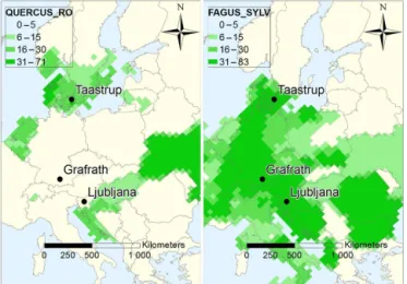
Figure 1. European map over visited International Phenological Garden sites and the reported gridded tree density in percentage of English oak (left) and European beech (right). The sites used in this study are located in Slovenia (Ljubljana), Germany (Grafrath, 30 km W of Munich) and Denmark (Taastrup, 15 km W of Copen-hagen). The maps are redrawn from Skjøth et al. (2008), with per-mission.
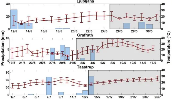
The long-term average air temperature and precipitation experienced on site generally decreased with increasing lat-itude (Table 1). The weather conditions for the visited sites differed during sampling (8:00–16:00 local time), where the daily precipitation and average temperature during the cam-paigns and two weeks prior to measurements can be found in Fig. 2. In Ljubljana, unstable weather conditions led to reoc-curring thunderstorms and average temperatures below 20◦C during the whole measurement campaign. In the beginning of the campaign in Grafrath, there were a couple of days with an average daily temperature between 12.4 and 14.3◦C be-fore it rose to an average of 21.2–24.5◦C. Clear, sunny con-ditions were experienced during the whole campaign with the exception of two short thunderstorms in the beginning of the measurement period. The highest temperature experi-enced reached up to 38.7◦C. Taastrup had one day of intense rainfall of 75 mm in the beginning of the campaign. The rest of the campaign experienced cloudy but calm weather with temperatures around 17.2–22.7◦C.
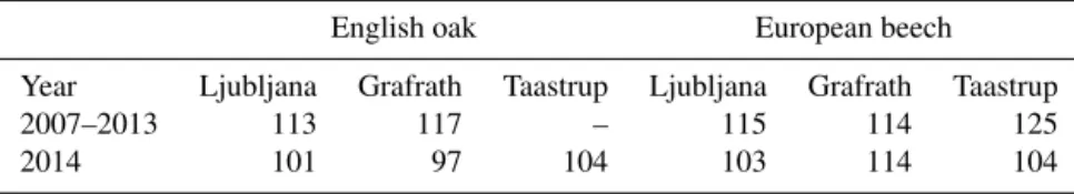
The leaf unfolding date for English oak and European beech was typically between 23 and 27 April for Ljubljana and Grafrath, whilst European beech in Taastrup unfolded its leaves 5 May. There are no long-term observational data for the leaf unfolding of English oak in Taastrup. In 2014, the leaf unfolding started 12–21 days earlier on all sites in com-parison to the long-term average for all trees. The exception was for the European beech in Grafrath, which followed the average time of unfolding (Table 2).
2.2 BVOC sampling and analysis, net assimilation and stomatal conductance
Measurements were made on five English oak trees (one in Ljubljana, two in Grafrath and two in Taastrup) and four Eu-ropean beech trees (one in Ljubljana, two in Grafrath and one in Taastrup). In Grafrath, only five year old English oaks were available, whilst the trees at the other sites were 42– 43 years old. For European beech, all trees were between 43 and 51 years old. Measurements were made on fully de-veloped leaves and one sample was taken per leaf. For En-glish oak, 5–9 leaves were measured per tree, giving a total of 36 samples. For European beech, 7–17 leaves were mea-sured per tree, which gives a total of 49 samples. All samples were taken on the lowest situated branches of the tree (1– 2 m above ground). This height was chosen as earlier results in Taastrup had shown little emission pattern difference for English oak and different heights within the tree due to the wide spacing between trees (Persson et al., 2016). Because there existed a similar wide spacing between trees in Ljubl-jana and Grafrath, sampling the lowest branches was consid-ered appropriate.
In addition to BVOC measurements, net assimilation rates (A) and stomatal conductance (gs) were determined for
each leaf using a portable photosynthesis system (LI-6400, LICOR, Lincoln, NE, USA), equipped with a LED source leaf chamber (6400-02B) and an external quantum sen-sor (LI-190SA) which measured daily photosynthetically active radiation (PAR) rates. The system allows control over CO2, light, temperature and humidity within the cham-ber, and the measurements were made under fixed environ-mental conditions. The leaf within the chamber was accli-mated to 1000 µmol m−2s−1PAR, 400 µmol CO
Figure 2.The daily precipitation (mm, blue) and average daily temperature (◦C, red) for IPG sites Ljubljana (Slovenia), Grafrath (Germany) and Taastrup (Denmark) two weeks prior (marked in white) and during measurement campaigns (marked in grey). The error bars mark the maximum and minimum temperatures during the day.
Table 1.Long-term monthly average temperature (◦C) and total monthly precipitation (mm) for Ljubljana in Slovenia, Grafrath in Germany and Taastrup in Denmark (averaging period is indicated).
Site Weather parameter May June July Yearly Time period Source
Ljubljana Temperature (◦C) 15.8 19.1 21.3 10.9 1981–2010 Slovenian Environmental Agency: http://meteo.arso.gov.si/
(last access: 10 October 2015) Precipitation (mm) 109 144 115 1362
Grafrath Temperature (◦C) 12.9 16.6 20.9 8.5 1995–2010 Agrarmeteorologie Bayern: http://www.wetter-by.de/ (last access: 9 October 2015) Precipitation (mm) 170.1 134.2 30.6 877
Taastrup Temperature (◦C) 11.7 14.8 17.5 8.7 1997–2010 Danish Meteorological Institute: dmi.dk
(last access: 12 October 2015) Precipitation (mm) 52 76.3 72.3 687
into the LI-6400 system (for further details on the equations used by the instrument, see von Caemmerer and Farqua-har, 1981). In order to get theA-Ci response, the CO2level was changed within the chamber. The CO2amount was first decreased from 400 to 100 µmol mol−1 in 100 µmol mol−1 steps and a further 50 µmol mol−1to reach the lowest level. The CO2level was then increased to 400 µmol mol−1, where two points were logged in a row to allow the leaf some recovery. Lastly, the CO2 level was increased to 1000 in 200 µmol mol−1steps. This resulted in 10 logged points. For each step, there was an adjustment time of at least 90 s in order to reach stability. If stability was not reached after 150 s, logging would occur anyway. The water use efficiency
(WUE) for the leaves was calculated by dividing the net assimilation rate with the transpiration rate. Lastly, the dry weight of the leaves was determined.
Table 2.The day of year (DOY) for leaf unfolding for English oak and European beech at sites Ljubljana, Grafrath and Taastrup, with both an average between 2007 and 2013 and the unfolding in 2014. No long-term observations for leaf unfolding of English oak in Taastrup are available.
English oak European beech
Year Ljubljana Grafrath Taastrup Ljubljana Grafrath Taastrup
2007–2013 113 117 – 115 114 125
2014 101 97 104 103 114 104
5◦C min−1and further up to 250◦C at a rate of 20◦C min−1. The BVOCs were separated using a HP-5 capillary column (50 m, diameter 0.2 mm and film thickness 0.33 µm). The compounds were identified according to pure standard so-lutions and the mass spectra in the Wiley data library (Wiley and Sons Ltd., Chichester, UK). Standard solutions were in-jected into adsorbent cartridges in a stream of helium and analysed as samples. The standards available were isoprene,
α-pinene, camphene,δ-phellandrene, limonene, eucalyptol, γ-terpinene, linalool, aromadendrene and α-humulene in
methanol (Fluka, Buchs, Switzerland). To quantify BVOCs to which no standards were available, α-pinene was used
for MTs and α-humulene was used for SQTs. All
chro-matograms were analysed with the MSD ChemStation Data Analysis software (G1701CA C.00.00 21 December 1999; Agilent Technologies, Santa Clara, CA, USA).
2.3 BVOC standardization
Since previous studies have shown that both English oak and European beech have light- and temperature-dependent emissions (Niinemets et al., 2004; Dindorf et al., 2006; De-marcke et al., 2010; Kleist et al., 2012), all emission rates were standardized according to the temperature- and light-dependent model of Guenther et al. (1993, 1995). The Eq. (1) is as follows:
I =IS·CL·CT, where CL=
αCL1PAR
p
1+α2PAR2
and CT =
expCT1(T−TS) RTST 1+expCT2(T−TM)
RTST
, (1)
where I stands for isoprene emission rate at temperature T (K) and PAR flux (µmol m−2s−1) and IS is the iso-prene emission rate at a standard temperature TS (303 K) and a standard PAR flux (1000 µmol m−2s−1).C
L is a fac-tor for light dependence of the compound, whereα=0.0027
and CL1=1.066 are empirical coefficients. CT is a fac-tor for temperature dependency, where R is the
univer-sal gas constant (8.314 J K−1) and C
T1=95 000 J mol−1,
CT2=230 000 J mol−1andTM=314 K are empirical coef-ficients. The standardization was done in order to be able to compare samples which had experienced different daily tem-peratures. In our measurements, the same PAR conditions of 1000 µmol m−2s−1were used on all samples, resulting in
CL1=1. Temperature varied between 293 and 304 K andIS was determined by combining the observedI and the
com-putedCT.
2.4 Statistical analysis
A one way Analysis of Variance (ANOVA) followed by Tukey’s test was performed to test if the total BVOC emis-sions differed between sites and a two-sample t test was
made to test for similarities between clones from the same site.
Principal component analysis (PCA) was used in order to investigate whether the individual trees differed from each other within and between sites according to their individual BVOC emission patterns. The PCA was run through SIMCA (Umetrics, version 13.0.3.0, Umeå, Sweden) after centring and unit variance-scaling of the variables. Two outliers from English oak with extremely high emissions were removed from the dataset due to suspected rough handling of the leaves.
3 Results
3.1 Photosynthetic rates andA-Ciresponses
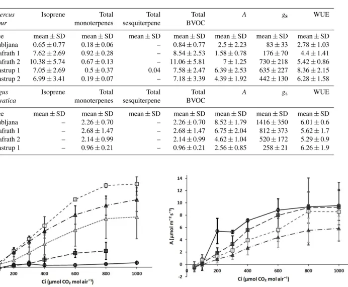
The net assimilation rate at standard CO2 conditions (400 µmol mol−1)for English oak ranged between 1.58 and 7.00 µmol CO2m−2s−1, with the lowest rates found in Ljubljana and one of the Grafrath trees and the highest rate found in the other Grafrath tree. Similarly, gsranged between 83 and 730 mmol H2O m−2s−1, with the lowest rates found in Ljubljana and the highest in the second tree growing in Grafrath. The WUE had a range of 2.78–8.36 µmol mol−1 (Table 3).
For European beech, the average net assimilation rate ranged between 2.56 and 8.93 µmol CO2m−2s−1, with the lowest rates in Taastrup and the highest rate in Ljubljana.gs
was between 258 and 1416 mmol H2O m−2s−1. The WUE did not vary considerably between sites, with a range of 5.29–6.00 µmol mol−1(Table 3).
In total, 3–4A-Ci curves were taken per tree for English oak and 3–10 for European beech. TheA-Ci curves for En-glish oak showed a similar pattern as with the net assimila-tion rate andgs, with less response from Ljubljana and one
Table 3.Standardized BVOC emission (µg gdw−1h−1), the net assimilation rate (A, µmol CO2m−2s−1), stomatal conductance (gs, mmol H2O m−2s−1)and Water Use Efficiency (WUE, µmol mol−1)for English oak tree clones and European beech tree clones at sites Ljubljana in Slovenia, Grafrath in Germany and Taastrup in Denmark. The values are averages from the samples collected from each tree and site±the standard deviation (SD). The hyphen indicates that there was no compound detected for the site and tree.
Quercus Isoprene Total Total Total A gs WUE
robur monoterpenes sesquiterpene BVOC
Tree mean±SD mean±SD mean±SD mean±SD mean±SD mean±SD mean±SD Ljubljana 0.65±0.77 0.18±0.06 – 0.84±0.77 2.5±2.23 83±33 2.78±1.03 Grafrath 1 7.62±2.69 0.92±0.28 – 8.54±2.53 1.58±0.78 176±70 4.4±1.41 Grafrath 2 10.38±5.74 0.67±0.13 – 11.06±5.81 7±1.25 730±218 5.42±0.86 Taastrup 1 7.05±2.69 0.5±0.37 0.04 7.58±2.47 6.39±2.53 635±227 8.36±2.15 Taastrup 2 6.99±3.41 0.19±0.07 – 7.18±3.39 4.39±1.92 442±130 6.28±1.58
Fagus Isoprene Total Total Total A gs WUE
sylvatica monoterpenes sesquiterpene BVOC
Tree mean±SD mean±SD mean±SD mean±SD mean±SD mean±SD mean±SD Ljubljana – 2.26±0.70 – 2.26±0.70 8.52±1.79 1416±350 6.01±0.6 Grafrath 1 – 2.68±1.47 – 2.68±1.47 6.75±2.04 812±373 5.62±1.7 Grafrath 2 – 2.14±0.99 – 2.14±0.99 4.62±1.04 520±172 5.29±0.9 Taastrup 1 – 0.96±0.21 – 0.96±0.21 2.56±0.85 258±21 6.26±1.9
Figure 3.Net assimilation rateAand intercellular CO2 concentra-tion (Ci)response curves for English oak. The figure represents the averageA-Ciresponse curves for each tree±SD.
tree in Grafrath and in Taastrup. There was a clear difference in the CO2 response between the trees in Grafrath, but no clear difference from the trees growing in Taastrup (Fig. 3). All the European beech trees showed a similar response with increasing CO2levels, where the net assimilation rate tended to level off at 800 µmol CO2mol air−1. Taastrup has the low-est CO2response in regards to different CO2levels, but with-out distinct differences from the other trees (Fig. 4).
3.2 BVOC emission from English oak and European beech
The ranges of the total standardized BVOC emission rates from the English oak and European beech trees differed
con-Figure 4.Net assimilation rateAand intercellular CO2 concentra-tion (Ci)response curves for European beech. The figure represents the averageA-Ciresponse curves for each tree±SD.
siderably between sites (Table 3). The English oak in Ljubl-jana had low emission with no high values, and the emis-sion was lower in comparison to the other sites (P <0.001 for
Tukey’s test). The highest emission variation was found for tree number two in Grafrath. One of the European beech trees in Grafrath had the highest emission variation, whilst the tree in Taastrup had the lowest variation and significantly lower emissions than the other sites (P <0.01). For both English
oak and European beech, the total BVOC emissions from the cloned trees from the same site were not significantly differ-ent from each other (P >0.05).
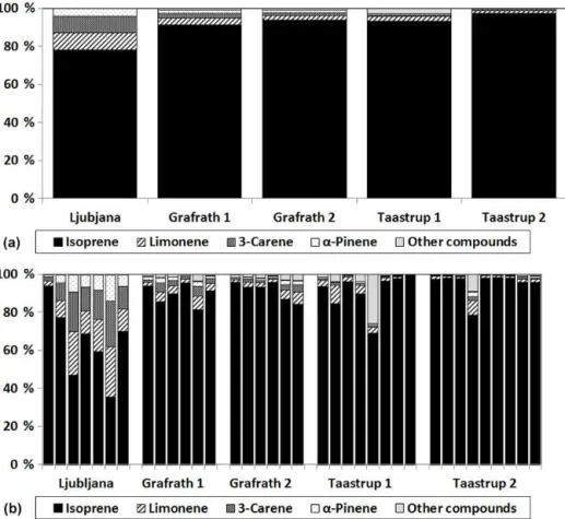
Figure 5.Relative BVOC compound contribution from English oak seen as(a)sample averages for different trees and sites and(b)for
individual samples. The major emitted compounds are presented separately, whilst the remaining compounds are classified into other com-pounds.
11.06 µg gdw−1h−1, with the highest emissions in Grafrath and the lowest emissions in Ljubljana. The largest contribu-tion to the overall emission came from isoprene, which made up 78–97 % of the total BVOC emission (Table 3). Each sam-ple contained between 3 and 6 detectable compounds which, apart from isoprene, were α-pinene, camphene, 3-carene,
limonene andβ-ocimene.
The mature oak in Ljubljana had lowest emissions, rang-ing from 0.18 to 2.65 µg gdw−1h−1between samples. From the two five-year-old trees in Grafrath, the emission rate ranged between 4.32 and 12.49 µg gdw−1h−1 for the first oak and between 2.62 and 20.12 µg gdw−1h−1 for the sec-ond oak. In Taastrup, the emission rate ranged from 4.99 to 11.41 µg gdw−1h−1for the first mature oak and between 1.6 and 12.6 µg gdw−1h−1for the second oak.
The European beech had an average emission rate be-tween 0.96 and 2.68 µg gdw−1h−1, with the highest emis-sion found at the site in Grafrath and the lowest emisemis-sion in Taastrup. The total emission rate was fairly similar in both Ljubljana and Grafrath, with a range of emission of 1.35– 3.43 µg gdw−1h−1 in Ljubljana and 0.3–5.7 µg gdw−1h−1 in Grafrath. Taastrup had the lowest standard emission rate, ranging from 0.62 to 1.36 µg gdw−1h−1 (Table 3).
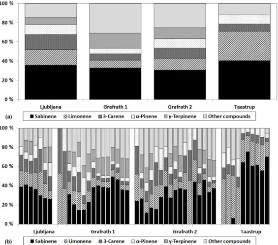
Each sample contained between 2 and 10 detectable pounds. In addition to sabinene, which had the highest com-pound contribution, these were α-thujene, α-pinene,
cam-phene,α-phellandrene, 3-carene,α-terpinene, limonene,β
-phellandrene,γ-terpinene and terpinolene.
3.3 Compound variation across latitudes
Both the individual samples and the relative emission con-tribution of major emitted compounds varied between sites for both English oak and European beech (Figs. 5 and 6). For English oak, the percentage of compound contribution from isoprene varied between 91 and 97 % apart from the tree growing in Ljubljana where the contribution was 78 %. In Ljubljana there was a higher variation between samples in comparison to the other sites, where a few samples had high isoprene emission whilst the remaining samples con-tained more monoterpenes. Other major emitted compounds were limonene, 3-carene andα-pinene (in decreasing order),
Figure 6.Relative BVOC compound contribution from European beech seen as(a)sample averages for different trees and sites and(b)
for individual samples. The major emitted compounds are presented separately, whilst the remaining compounds are classified into other compounds.
In the few samples where sabinene had not been detected, limonene was the main emitted compound. In Grafrath, these samples were taken usually before 09:00 LT in the morn-ing. For the tree in Taastrup, the samples without sabinene were from leaves which were more yellow in colour than the other leaves. The remaining compounds varied in importance depending on the site. γ-Terpinene was an important
com-pound in Ljubljana and Grafrath, but not emitted at all in Taastrup. Taastrup also had the highest relative contribution of sabinene within samples, when it was emitted, and less compound variation in comparison to the other cloned trees (Fig. 6).
PCA was used to describe latitudinal differences based upon the BVOC emission profiles (Figs. 7 and 8). The En-glish oak trees showed a clear separation between sites, but less within (Fig. 7). The first PC explained 60.9 % of the vari-ation in the emission of individual BVOCs and it separated the samples from Grafrath from Ljubljana and Taastrup. It also described the difference in emission profiles with re-gard to the average daily temperature, where high temper-atures were found towards the right of the graph. The sec-ond PC explained 18.0 % of the variation and separated the
samples from Ljubljana and Taastrup. The emission profiles within a site were not separated from each other. The average daily PAR did not correlate with the emission profiles. The loading plot revealed that the Grafrath samples were char-acterized by higher relative emissions of other compounds than the monoterpeneβ-ocimene, which was a characteristic
compound for Taastrup (Fig. 7).
Figure 7.Principal component analysis on the BVOC emission from five cloned English oak trees grown at three sites.(a)The scores of the
principal components (PC1 and PC2), and(b)the corresponding loading variables. In(a), the shading explains the average air temperature. The size of the symbols depicts the average daily PAR level, with an increasing symbol size with increasing PAR levels. The symbols show samples from the different sites (circle=Ljubljana, square=Grafrath tree one, triangle=Grafrath tree two, diamond=Taastrup tree one and pentagon=Taastrup tree two). The explained variance for the different PCs is shown in parentheses.
Figure 8.Principal component analysis on the BVOC emission from four cloned individual European beech trees growing at three sites. (a)The scores of the principal components (PC1 and PC2), and(b)the corresponding loading variables. In(a), the shading explains the average air temperature. The size of the symbols depicts the average daily PAR level, with an increasing symbol size with increasing PAR levels. The symbols show samples from the different sites (circle=Ljubljana, square=Grafrath tree one, triangle=Grafrath tree two, diamond=Taastrup). The explained variance for the different PCs is shown in parentheses.
4 Discussion
The amount emitted and the mixture of BVOCs reported in the literature can vary immensely for individual species (Kesselmeier and Staudt, 1999; Owen et al., 2001; Noe et al., 2012; Pokorska et al., 2012; Steinbrecher et al., 2013). Some studies suggest that this within-species variability is mostly due to genetic variation, but the majority of studies performed have either done measurements on mature and ge-netically different trees or on gege-netically identical but young and potted individuals (Lehning et al., 1999; Staudt et al., 2001; Funk et al., 2005; Bäck et al., 2012). One of the aims of this campaign was to study if similar emission patterns were observed for genetically identical individuals in order to further confirm this genetic dependency. By using the IPG network, where common European tree species are cloned
and dispersed across Europe, it is possible to measure the emission pattern variability under natural field conditions for the same genotype grown at different locations. And as the network has been in practice since 1957 (Chmielewski et al., 2013), many of the sites could provide mature trees, which often have different BVOC emission rates and patterns in comparison to younger trees (Street et al., 1997; Csiky and Seufert, 1999; Thoss et al., 2007).
did not provide significantly different emission profiles. We also showed that the main compounds emitted from English oak and European beech were the same at different sites, al-though there were some differences in the relative contribu-tion. The most dominant compounds released were isoprene for English oak and sabinene for European beech which is in line with previous studies (Isidorov et al., 1985; Tollsten and Müller, 1996; Kesselmeier and Staudt., 1999; Dindorf et al., 2006; Holzke et al., 2006; Kleist et al., 2012; Pokorska et al., 2012; Steinbrecher et al., 2013; Persson et al., 2016).
4.1 BVOC emission in regards to local growing conditions
The average standardized emission for English oak was be-tween 0.84 and 11.06 µg gdw−1h−1, which is a low estimate compared with other studies (Isidorov et al., 1985; König et al., 1995; Kesselmeier and Staudt, 1999; Pokorska et al., 2012 and references within; Persson et al., 2016). The low-est emission came from Ljubljana, which was expected to have the highest BVOC emission rate due to its southern lo-cation. However, the oak tree was severely damaged by a frost event in the beginning of the year prior to the measure-ments, and a third of the tree had to be cut in order to save it (A. Žust, personal communication, 2014). Both the frost and the cutting would have caused stress to the tree, and it is most likely that most resources would be allocated to re-covery rather than BVOC emissions. A low net assimilation rate of 2.5 µmol CO2m−2s−1 also indicated stress, which was less than half the rates found at the other sites, apart from one of the Grafrath trees. The assimilation rates of the tree in Ljubljana and Grafrath 1 correspond to the assimila-tion rates reported from shade-adapted leaves, whilst the re-maining rates are in range of sun-adapted leaves (Morecroft and Roberts, 1999; Vallandres et al., 2002). Furthermore, gs, WUE and theA-Ciresponse were also low during the time of sampling, indicating closed stomata and low photosynthetic activity within the leaves. A similar pattern was shown for one of the young trees growing in Grafrath, which is also re-flected in the lower BVOC emission capacity compared with the other clone growing at the same site (Fig. 3 and Table 3). At Grafrath, there were only young English oak trees avail-able for performing measurements as the only fully grown tree had died a couple of years earlier (Martin Piepenburg, personal communication, 2014). As the emission rates may vary with the age of the tree (Street et al., 1997; Thoss et al., 2007), the age difference should be taken into account when the total emission rates are compared between sites. However, as the relative emission spectra remained stable be-tween sites, it is likely when compared to the study made by Street et al. (1997) that an adult tree from Grafrath would emit a similar compound spectrum in comparison to the trees measured in this study.
The average standardized emission for European beech ranged between 0.96 and 2.68 µg gdw−1h−1, which is low
or within range of other studies (Tollsten and Müller, 1996; Moukhtar et al., 2005; Holzke et al., 2006 and references therein). One reason for the low emission rates in this study could be that all the measurements were performed at the bottom part of the canopy. The beech in Taastrup has been shown to have a clear vertical emission profile, where the top of the canopy emitted 7–9 times more in comparison to lower levels of the tree (Persson et al., 2016).
Another reason for the low emission rates could be the ef-fect of other climatic influences than temperature and PAR. Beech is particularly drought sensitive and prone to adap-tation depending on the local climatic conditions (Peuke et al., 2002). In this study, the average net assimilation rate for Ljubljana and Grafrath were between 4.62 and 8.93 µmol CO2m−2s−1, whilst Taastrup had the lowest rate of 2.56 µmol CO2 m−2s−1. The values for Ljubljana and Grafrath are in the same range as assimilation rates for sun-lit leaves, whilst values from Taastrup are more similar to the assimilation rate for shaded leaves (Warren et al., 2007). In comparison to Ljubljana and Grafrath, the leaves in Taas-trup were yellower in colour which might suggest some type of stress within the tree. Even though the net assimilation rate andgswere lower in Taastrup in comparison to the other sites, there was no clear difference in their WUE. Both the net assimilation rate and the transpiration rate followed a simi-lar increasing or decreasing pattern, resulting in fairly stable WUE levels. This might be due to an ecotype adaptation sug-gested by Peuke et al. (2002), but longer and more detailed studies need to be conducted to confirm this hypothesis.
Even though studies have suggested that genetic varia-tion has a strong influence on the BVOC emission patterns (Staudt et al., 2001; Funk et al., 2005; Bäck et al., 2012), local meteorological conditions are also expected to affect emission characteristics. It is well known that light and tem-perature have an important impact on plant BVOC emissions (see review by Grote et al., 2013; Li and Sharkey, 2013), but other factors such as soil moisture, nutrient availability and biotic influences (e.g. herbivory) can further influence the emission patterns (Kesselmeier and Staudt, 1999; Peñuelas and Llusià, 2001; Possell et al., 2004; Wu et al., 2015).
showed even less clear distinctions between samples and sites (see Figs. 7 and 8). This would suggest a more com-plex interaction between weather and the local growing con-ditions, which was not be assessed in this study. Therefore, more studies are needed with more cloned individual trees and over different growing seasons in order to confirm this weather dependency.
4.2 Uncertainties
In this work, all measurements were conducted on the low-est positioned branches, as it was assumed to have little ef-fect on English oak due to the wide spacing between trees. In Taastrup it was concluded that the wide spacing between trees caused similar light conditions at different height levels, and therefore resulted in similar emission patterns (Persson et al., 2016). Other studies performed in denser forests have concluded that higher emissions are generally found at sun-lit leaves (Bertin et al., 1997; Harley et al., 1997; Šimpraga et al., 2013). Furthermore, for Grafrath which only had five-year-old trees with an approximate height of 1 m, the differ-ence between sunlit and shaded leaves was limited. However, as the trees in Ljubljana and Grafrath were standing with a comparable spacing between trees as the trees in Taastrup, we assume a similarly small difference between light inten-sities as were found in Taastrup in 2013. For European beech, it is more likely that there would have been an emission dif-ference between the upper and lower part of the canopy. This needs to be taken into consideration when regarding these figures. But as all the trees have been measured at approxi-mately the same height, it is still possible to make compar-isons between visited sites.
BVOC emission rates and spectra tend to differ over time. Holzke et al. (2006) measured a fully matured European beech tree over two vegetation periods to study the BVOC emission difference in time. Even though the tree experi-enced higher mean temperatures and longer warm periods, the emission rates measured in the latter year were lower than the former. It was explained to be caused by preceding weather events and in particular long periods without rainfall, which might have restricted leaf development. Leaf unfold-ing for European beech was approximately three weeks ear-lier in 2014 in comparison to 2013, but for both campaigns the beech leaves had at least 80 days to mature before mea-surements were taken. There are no leaf unfolding data for 2013 for English oak. When average temperatures and total amount of rainfall were compared, 2014 was a slightly wet-ter (+173 mm) and warmer (+2◦C) year in comparison to
2013 seen over the whole year. During the period between May and July where measurements were taken, the weather did not differ considerably between 2013 and 2014 (data not shown). But when the emission rates from this study were compared with the emission rates in Taastrup (for more in-formation, see Persson et al., 2016), the emission rates in 2013 were ten times higher for European beech in
compar-ison to 2014. In this case, past weather events do not ex-plain the huge variation in BVOC emissions between the two measured years. However, the composition of compounds remained fairly stable, which could be an important aspect when it comes to modelling. This stability in the emission spectra has been seen for other trees as well (Staudt et al., 2001; Bäck et al., 2012), but the stability has usually only been tested over a few years. In order to prove that emission spectra remain stable over time, more studies over longer pe-riods of time need to be done.
5 Conclusions
This work both highlights the potential stability in BVOC emission spectra across regions and discusses the climatic impact on English oak and European beech on trees that lack genetic variation. The IPG network, which studies the phe-nological patterns from genetically identical European tree species, has been used in order to better understand intraspe-cific variation between sites and the causes behind them. The work further emphasizes the need to perform studies over longer timescales in order to fully understand the emission pattern variation.
Despite differences in age and location, the relative contri-butions of the highest emitted compounds were stable within as well as between studied sites in the latitudinal transect. However, the amounts of BVOC released differed between sites, even when standardized (Guenther et al., 1993, 1995) to the same temperature and light levels. This is most likely caused by past weather events and stress such as frost dam-age and tree cutting. The BVOC emission measured for En-glish oak and European beech was lower than previous mea-surements by other studies, but the lower BVOC emission amounts were consistent for all sites and trees. Restricted photosynthetic production, stomatal conductance and CO2 response of the leaves further suggest stress for some of the trees.
6 Data availability
The data set related to this study has been provided as a sup-plement.
The Supplement related to this article is available online at doi:10.5194/bg-13-6067-2016-supplement.
Acknowledgements. We thank Ana Žust (Environmental agency
of the Republic of Slovenia), Martin Piepenburg (Bavarian State Institute of Forestry) and Anders Kristian Nørgaard (University of Copenhagen) for their assistance during field campaigns and Frank M. Chmielewski (Humboldt University of Berlin) for help and information about the IPG network. We thank Magnus Kramshøj and Michelle Schollert for performing the GC-MS analysis. Lastly, we thank Carsten Skjøth for providing species distribution data for English oak and European beech in Europe and Max van Meeningen for compiling the data into maps. The study was performed within the framework of LUCCI, which is a research centre at Lund University for studies of carbon cycles and climate interaction. Support from the Swedish Research Council VR and FORMAS are acknowledged.
Edited by: X. Wang
Reviewed by: two anonymous referees
References
Atkinson, R.: Atmospheric chemistry of VOCs and NOx, Atmos. Environ., 34, 2063–2101, 2000.
Bäck, J., Aalto, J., Henriksson, M., Hakola, H., He, Q., and Boy, M.: Chemodiversity of a Scots pine stand and implica-tions for terpene air concentraimplica-tions, Biogeosciences, 9, 689–702, doi:10.5194/bg-9-689-2012, 2012, 2012.
Bertin, N., Staudt, M., Hansen, U., Seufert, G., Ciccioli, P., Fos-ter, P., Fugit, J. L., and Torres, L.: Diurnal and seasonal course of monoterpene emissions fromQuercus ilex(L.) under natural light and temperature algorithms, Atmos. Environ., 31, 135–144, 1997.
Chmielewski, F.-M., Heider, S., and Moryson, S.: International Phe-nological Observation Networks: Concept of IPG and GPM, in: Phenology: An Integrative Environmental Science, edited by: Schwartz, M. D., Springer Science+Business Media B.V., 137– 153, doi:10.1007/978-94-007-6925-0_8, 2013.
Csiky, O. and Seufert, G.: Terpenoid emissions of Mediterranean oaks and their relation to taxonomy, Ecol. Appl., 9, 1138–1146, 1999.
Demarcke, M., Müller, J.-F., Schoon, N., Van Langenhove, H., Dewulf, J., Joó, E., Steppe, K., Šimpraga, M., Heinesch, B., Aubinet, M., and Amelynck, C.: History effect of light and tem-perature on monoterpenoid emissions fromFagus sylvaticaL.,
Atmos. Environ., 44, 3261–3268, 2010.
Di Carlo, P., Brune, W. H., Martinez, M., Harder, H., Lesher, R., Ren, X., Thornberry, T., Carroll, M. A., Young, V., Shepson, P.
B., Riemer, D., Apel, E., and Campbell, C.: Missing OH reac-tivity in a forest: evidence for unknown reactive biogenic VOCs, Science, 304, 722–725, 2004.
Dindorf, T., Kuhn, U., Ganzeveld, L., Schebeske, G., Ciccioli, P., Holzke, C., Köble, R., Seufert, G., and Kesselmeier, J.: Signif-icant light and temperature dependent monoterpene emissions from European beech (Fagus sylvaticaL.) and their potential
im-pact on the European volatile organic compound budget, J. Geo-phys. Res., 111, 1–15, doi:10.1029/2005JD006751, 2006. Ekberg, A., Arneth, A., Hakola, H., Hayward, S., and Holst, T.:
Iso-prene emission from wetland sedges, Biogeosciences, 6, 601– 613, doi:10.5194/bg-6-601-2009, 2009.
Funk, J. L., Jones, C. G., Gray, D. W., Throop, H. L., Hyatt, L. A., and Lerdau, M. T.: Variation in isoprene emission fromQuercus rubra?: Sources, causes, and consequences for estimating fluxes,
J. Geophys. Res., 110, D04301, doi:10.1029/2004JD005229, 2005.
Grote, R., Monson, R. K., and Niinemets, Ü.: Leaf-level models of constitutive and stress-driven volatile organic compound emis-sions, in: Biology, controls and models of tree volatile organic compound emissions, edited by: Niinemets, Ü. and Monson, R. K., Springer Netherlands, 315–355, 2013.
Guenther, A. B., Zimmerman, P. R., Harley, P. C., Monson, R. K., and Fall, R.: Isoprene and monoterpene emission rate variability: Model evaluations and sensitivity analyses, J. Geophys. Res., 98, 12609–12617, 1993.
Guenther, A., Hewitt, C. N., Erickson, D., Fall, R., Geron, C., Graedel, T., Harley, P., Klinger, L., Lerdau, M., McKay, W. A., Pierce, T., Scholes, B., Steinbrecher, R., Tallamraju, R., Taylor, J., and Zimmerman, P.: A global model of natural volatile organic compound emissions, J. Geophys. Res., 100, 8873–8892, 1995. Harley, P., Guenther, A., and Zimmerman, P.: Environmental
con-trols over isoprene emission in deciduous oak canopies, Tree Physiol., 17, 705–714, 1997.
Holopainen, J. K.: Can forest trees compensate for stress-generated growth losses by induced production of volatile compounds?, Tree Physiol., 31, 1356–1377, 2011.
Holzke, C., Dindorf, T., Kesselmeier, J., Kuhn, U., and Koppmann, R.: Terpene emissions from European beech (Fagus sylvaticaL.):
pattern and emission behaviour over two vegetation periods, J. Atmos. Chem., 55, 81–102, 2006.
Isidorov, V. A., Zenkevich, I. G., and Ioffe, B. V.: Volatile Organic Compounds in the atmosphere of forests, Atmos. Environ., 19, 1–8, 1985.
Karl, M., Guenther, A., Köble, R., Leip, A., and Seufert, G.: A new European plant-specific emission inventory of biogenic volatile organic compounds for use in atmospheric transport models, Bio-geosciences, 6, 1059–1087, doi:10.5194/bg-6-1059-2009, 2009. Kesselmeier, J. and Staudt, M.: Biogenic Volatile Organic Com-pounds (VOC): An overview on emission, physiology and ecol-ogy, Atmos. Chem., 33, 23–88, 1999.
Kleist, E., Mentel, T. F., Andres, S., Bohne, A., Folkers, A., Kiendler-Scharr, A., Rudich, Y., Springer, M., Tillmann, R., and Wildt, J.: Irreversible impacts of heat on the emissions of monoterpenes, sesquiterpenes, phenolic BVOC and green leaf volatiles from several tree species, Biogeosciences, 9, 5111– 5123, doi:10.5194/bg-9-5111-2012, 2012.
hydro-carbons to the total biogenic VOC emissions of selected mid-European agricultural and natural plant species, Atmos. Envir., 29, 861–874, 1995.
Kost, C. and Heil, M.: Herbivore-induced plant volatiles induce an indirect defence in neighbouring plants, J. Ecol., 94, 619–628, 2006.
Langenheim, J. H.: Higher plant terpenoids: a phytocentric overview of their ecological roles, J. Chem. Ecol., 20, 1223– 1280, 1994.
Laothawornkitkul, J., Taylor, J. E., Paul, N. D.. and Hewitt, C. N.: Biogenic volatile organic compounds in the Earth system, New Phytol., 183, 27–51, 2009.
Lehning, A., Zimmer, I., Steinbrecher, R., Brüggemann, N., and Schnitzler, J.-P.: Isoprene synthase activity and its relation to iso-prene emission inQuercus roburL. leaves, Plant Cell Environ.,
22, 495–504, 1999.
Lerdau, M., Guenther, A., and Monson, R.: Plant Production Emis-sion of Volatile Organic Compounds, BioScience, 47, 373–383, 1997.
Li, Z. and Sharkey, T. D.: Molecular and pathway controls on bio-genic volatile organic compound emissions, in: Biology, controls and models of tree volatile organic compound emissions, edited by: Niinemets, Ü and Monson R. K., Springer Netherlands, 119– 150, 2013.
Maffei, M. E.: Sites of synthesis, biochemistry and functional role of plant volatiles, S. Afr. J. Bot., 76, 612–631, 2010.
Morecroft, M. D. and Roberts, J. M.: Photosynthesis and Stom-atal Conductance of Mature Canopy Oak (Quercus robur) and Sycamore (Acer pseudoplatanus) Trees Throughout the Growing Season, Funct. Ecol., 13, 332–342, 1999.
Moukhtar, S., Bessagnet, B., Rouil, L., and Simon, V.: Monoter-pene emissions from Beech (Fagus sylvatica) in a French forest
and impact on secondary pollutants formation at regional scale, Atmos. Environ., 39, 3535–3547, 2005.
Niinemets, Ü., Loreto, F., and Reichstein, M.: Physiological and physicochemical controls on foliar volatile organic compound emissions, Trends Plant Sci., 9, 180–186, 2004.
Noe, S. M., Hüve, K., Niinemets, Ü., and Copolovici, L.: Sea-sonal variation in vertical volatile compounds air concentrations within a remote hemiboreal mixed forest, Atmos. Chem. Phys., 12, 3909–3926, doi:10.5194/acp-12-3909-2012, 2012.
Oderbolz, D. C., Aksoyoglu, S., Keller, J., Barmpadimos, I., Stein-brecher, R., Skjøth, C. A., Plaβ-Dülmer, C., and Prévôt, A. S. H.: A comprehensive emission inventory of biogenic volatile organic compounds in Europe: improved seasonality and land-cover, Atmos. Chem. Phys., 13, 1689–1712, doi:10.5194/acp-13-1689-2013, 2013.
Owen, S. M., Boissard, C., and Hewitt, C. N.: Volatile organic com-pounds (VOCs ) emitted from 40 Mediterranean plant species: VOC speciation and extrapolation to habitat scale, Atmos. En-vir., 35, 5393–5409, 2001.
Paasonen, P., Asmi, A., Petäjä, T., Kajos, M. K., Äijälä, M., Jun-ninen, H., Holst, T., Abbatt, J. P. D., Arneth, A., Birmili, W., van der Gon, H. G., Hamed, A., Hoffer, A., Laakso, L., Laakso-nen, A., Leaitch, W. R., Plass-Dülmer, C., Pryor, S. C., RäisäLaakso-nen, P., Swietlicki, E., Wiedensohler, A., Worsnop, D. R., Kerminen, V.-M., and Kulmala, M.: Warming-induced increase in aerosol number concentration likely to moderate climate change, Nat. Geosci., 6, 438–442, 2013.
Peñuelas, J. and Llusià, J.: The complexity of factors driving volatile compound emissions by plants, Biol. Plantarum, 44, 481–487, 2001.
Peñuelas, J. and Staudt, M.: BVOCs and global change, Trends Plant Sci., 15, 133–144, 2010.
Persson, Y., Schurgers, G., Ekberg, A., and Holst, T.: Effects of intra-genotypic variation, variance with height and time of sea-son on BVOC emissions, Meteorol. Z., 25, 377–388, 2016. Peuke, A. D., Schraml, C., Hartung, W., and Rennenberg H.:
Iden-tification of drought-sensitive beech ecotypes by physiological parameters, New Phytol., 154, 373–387, 2002.
Pierik, R., Ballaré, C. L., and Dicke, M.: Ecology of plant volatiles: taking a plant community perspective, Plant Cell Environ., 37, 1845–1853, 2014.
Pokorska, O., Dewulf, J., Amelynck, C., Schoon, N., Joó, É., Šim-praga, M., Bloemen, J., Steppe, K., and Van Langenhove, H.: Emissions of biogenic volatile organic compounds from Frax-inus excelsiorandQuercus roburunder ambient conditions in
Flanders (Belgium), Int. J. Environ. An. Ch., 92, 1729–1741, 2012.
Possell, M., Heath, J., Hewitt, C. N., Ayres, E., and Kerstiens, G.: Interactive effects of elevated CO2and soil fertility on isoprene emissions fromQuercus robur, Glob. Change Biol., 10, 1835–
1843, 2004.
Schurgers, G., Arneth, A., and Hickler, T.: Effect of climate-driven changes in species composition on regional emission capaci-ties of biogenic compounds, J. Geophys. Res., 116, D22304, doi:10.1029/2011JD016278, 2011.
Sharkey, T. D. and Yeh, S.: Isoprene emission from plants, Annu. Rev. Plant Physiol. Plant Mol. Biol., 52, 407–436, 2001. Sharkey, T. D., Singsaas, E. L., Lerdau, M. T., and Geron, C. D.:
Weather effects on isoprene emission capacity and applications in emissions algorithms, Ecol. Appl., 9, 1132–1137, 1999. Šimpraga, M., Verbeeck, H., Demarcke, M., Joó, É., Pokorska,
O., Amelynck, C., Schoon, N., Dewulf, J., Van Langenhove, H., Heinesch, B., Aubinet, M., Laffineur, Q., Müller, J.-F., and Steppe, K.: Clear link between drought stress, photosynthesis and biogenic volatile organic compounds inFagus sylvaticaL.,
Atmos. Environ., 45, 5254–5259, 2011.
Šimpraga, M., Verbeeck, H., Bloemen, J., Vanhaecke, L., Demar-cke, M., Joó, E., Pokorska, O., Amelynck, C., Schoon, N., Dewulf, J., Van Langenhove, H., Heinesch, B., Aubinet, M., and Steppe, K.: Vertical canopy gradient in photosynthesis and monoterpenoid emissions: An insight into the chemistry and physiology behind, Atmos. Environ., 80, 85–95, 2013.
Simpson, D., Winiwarter, W., Börjesson, G., Cinderby, S., Ferreiro, A., Guenther, A., Hewitt, C. N., Janson, R., Khalil, M. A. K., Owen, S., Pierce, T. E., Puxbaum, H., Shearer, M., Skiba, U., Steinbrecher, R., Tarrasón, L., and Öquist, M. G.: Inventorying emissions from nature in Europe, J. Geophys. Res., 104, 8113– 8152, 1999.
Skjøth, C. A., Geels, C., Hvidberg, M., Hertel, O., Brandt, J., Frohn, L. M., Hansen, K. M., Hedegård, G. B., Christensen, J. H., and Moseholm, L.: An inventory of tree species in Europe – an es-sential data input for air pollution modelling, Ecol. Model., 217, 292–304, 2008.
Staudt, M., Mandl, N., Joffre, R., and Rambal, S.: Intraspecific variability of monoterpene composition emitted byQuercus ilex
Steinbrecher, R., Contran, N., Gugerli, F., Schnitzler, J. -P., Zim-mer, I., Menard, T., and Günthardt-Goerg, M. S.: Inter- and intra-specific variability in isoprene production and photosynthesis of Central European oak species, Plant Biol., 15, 148–156, 2013. Street, R. A., Owen, S., Duckham, S. C., Boissard, C., and Hewitt,
C. N.: Effect of habitat and age on variations in volatile organic compounds (VOC) emissions fromQuercus ilexandPinus pinea,
Atmos. Environ., 31, 89–100, 1997.
Thoss, V., O’Reilly-Wapstra, J., and Iason, G. R.: Assessment and implications of intraspecific and phenological variability in monoterpenes of Scots pine (Pinus sylvestris) foliage, J. Chem.
Ecol., 33, 477–91, 2007.
Tollsten, L. and Müller, P. M.: Volatile organic compounds emitted from beech leaves, Phytochemistry, 43, 759–762, 1996.
Valladares, F., Manuel, J., Aranda, I., Balaguer, L., and Dizen-gremel, P.: The greater seedling high-light tolerance ofQuercus roburover Fagus sylvaticais linked to a greater physiological plasticity, Trees, 16, 395–403, 2002.
von Caemmerer, S. and Farquhar, G. D.: Some relationships be-tween the biochemistry of photosynthesis and the gas exchange of leaves, Planta, 153, 376–387, 1981.
Warren, C. R., Matyssek, R., and Tausz, M.: Internal conductance to CO2transfer of adultFagus sylvatica: Variation between sun
and shade leaves and due to free-air ozone fumigation, Environ. Exp. Bot., 59, 130–138, 2007.