Emissions from biomass burning in the Yucatan

(1)

ACPD

9, 767–836, 2009

Emissions from biomass burning in

the Yucatan

R. Yokelson et al.

Title Page

Abstract Introduction

Conclusions References

Tables Figures

◭ ◮

Back Close

Full Screen / Esc

Printer-friendly Version

Interactive Discussion

Atmos. Chem. Phys. Discuss., 9, 767–836, 2009 www.atmos-chem-phys-discuss.net/9/767/2009/ © Author(s) 2009. This work is distributed under the Creative Commons Attribution 3.0 License.

Atmospheric Chemistry and Physics Discussions

This discussion paper is/has been under review for the journalAtmospheric Chemistry and Physics (ACP). Please refer to the corresponding final paper inACPif available.

Emissions from biomass burning in the

Yucatan

R. Yokelson1, J. D. Crounse2, P. F. DeCarlo3,4, T. Karl5, S. Urbanski6, E. Atlas7, T. Campos5, Y. Shinozuka8, V. Kapustin8, A. D. Clarke8, A. Weinheimer5,

D. J. Knapp5, D. D. Montzka5, J. Holloway9, P. Weibring5, F. Flocke5, W. Zheng5, D. Toohey10, P. O. Wennberg11, C. Wiedinmyer5, L. Mauldin5, A. Fried5,

D. Richter5, J. Walega5, J. L. Jimenez12, K. Adachi13, P. R. Buseck13, S. R. Hall5, and R. Shetter5

1

University of Montana, Department of Chemistry, Missoula, MT 59812, USA 2

Division of Chemistry and Chemical Engineering, California Institute of Technology, Pasadena, USA

3

University of Colorado, Cooperative Institute for Research in the Environmental Sciences (CIRES), and Department of Atmospheric and Oceanic Sciences, Boulder, USA

4

Now at the Paul Scherrer Institut, Villigen Switzerland 5

National Center for Atmospheric Research, Boulder, CO, USA 6

USDA Forest Service, Fire Sciences Laboratory, Missoula, MT, USA 7

University of Miami, Rosenstiel School of Marine and Atmospheric Science, USA 8

(2)

ACPD

9, 767–836, 2009

the Yucatan

R. Yokelson et al.

Title Page

Tables Figures

◭ ◮

Back Close

Full Screen / Esc

9

NOAA ESRL/CSD, Boulder, CO, USA 10

University of Colorado, Department of Atmospheric and Oceanic Sciences, Boulder, USA 11

Divisions of Engineering and Applied Science and Geological and Planetary Science, Cali-fornia Institute of Technology, Pasadena, USA

12

University of Colorado, Cooperative Institute for Research in the Environmental Sciences (CIRES) and Department of Chemistry and Biochemistry, Boulder, USA

13

School of Earth and Space Exploration and Department of Chemistry and Biochemistry, Ari-zona State University, Tempe, USA

Received: 2 October 2008 – Accepted: 22 October 2008 – Published: 9 January 2009

(3)

ACPD

9, 767–836, 2009

the Yucatan

R. Yokelson et al.

Title Page

Tables Figures

◭ ◮

Back Close

Full Screen / Esc

Abstract

In March 2006 two instrumented aircraft made the first detailed field measurements of biomass burning (BB) emissions in the Northern Hemisphere tropics as part of the MILAGRO project. The aircraft were the National Center for Atmospheric Research C-130 and a University of Montana/US Forest Service Twin Otter. The initial emissions

5

of up to 49 trace gas or particle species were measured from 20 deforestation and crop residue fires on the Yucatan peninsula. This included two trace gases useful as indicators of BB (HCN and acetonitrile) and several rarely, or never before, measured species: OH, peroxyacetic acid, propanoic acid, hydrogen peroxide, methane sulfonic acid, and sulfuric acid. Crop residue fires emitted more organic acids and ammonia

10

than deforestation fires, but the emissions from the main fire types were otherwise fairly similar. The Yucatan fires emitted unusually high amounts of SO2and particle chloride,

likely due to a strong marine influence on this peninsula. As smoke from one fire aged, the ratio_∆O₃/∆CO increased to∼15% in <∼1 h similar to the fast net production of

O3 in BB plumes observed earlier in Africa. The rapid change in O3 occurs at a finer 15

spatial scale than is employed in global models and is also faster than predicted by micro-scale models. Fast increases in PAN, H₂O₂, and two organic acids were also observed. The amount of secondary organic acid is larger than the amount of known precursors. Rapid secondary formation of organic and inorganic aerosol was observed with the ratio_∆PM₂_.₅/∆CO more than doubling in∼1.4±0.7 h. The OH measurements 20

revealed high initial OH levels>1×107molecules/cm3. Thus, more research is needed to understand critical post emission processes for the second-largest trace gas source on Earth. It is estimated that∼44 Tg of biomass burned in the Yucatan in the spring of

2006. Mexican BB (including Yucatan BB) and urban emissions from the Mexico City area can both influence the March–May air quality in much of Mexico and the US.

(4)

ACPD

9, 767–836, 2009

the Yucatan

R. Yokelson et al.

Title Page

Tables Figures

◭ ◮

Back Close

Full Screen / Esc

1 Introduction

The MILAGRO (MegacityInitiative Local andGlobalResearchObservations) project was designed to study the local to global atmospheric affects of pollution from megacities (http://www.eol.ucar.edu/projects/milagro). Megacities have a population

>10 million and are rapidly increasing in number on the five most populated continents.

5

The first MILAGRO field campaigns occurred in March 2006 and studied the impact of trace gases and particles generated in Mexico City (MC, North America’s largest metropolitan area) on regional atmospheric chemistry (Fast et al., 2007; Molina et al., 2007). Regional biomass burning (BB) was also studied because it is a major emission source in Mexico that peaks during the February–May dry season. Earlier papers

esti-10

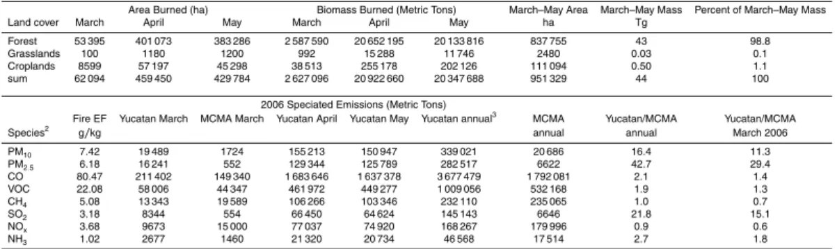
mated that BB located adjacent to MC accounted for∼20−30% of the CO (and several other important trace gases) and about one-half of the particle mass in the March 2006 MC outflow (Yokelson et al., 2007a; J. Crounse private communication). Another very important source of BB emissions in the MILAGRO study region is the Yucatan, which accounts for 7% of Mexico’s land area, but almost 30% of the total biomass burned

15

in Mexico annually (2002–2006 average) and almost 40% of the biomass burned in Mexico in 2006. (Section 4 describes the model used to generate these estimates.) From the perspective of the MILAGRO campaign, Yucatan BB emissions are important because MC and the Yucatan impact nearly the same regional environment and Yu-catan emissions can be transported to MC or interact with the MC plume downwind of

20

the city. For example, in 1998 intense BB in the Yucatan impacted air quality in much of Mexico and the US (Kreidenweis et al., 2001).

Yucatan BB is also of interest beyond the scope of the MILAGRO campaign. On a global basis, BB is the largest source of primary fine carbonaceous particles, the sec-ond largest source of trace gases, and it occurs mostly in the tropics, which play a

criti-25

(5)

ACPD

9, 767–836, 2009

the Yucatan

R. Yokelson et al.

Title Page

Tables Figures

◭ ◮

Back Close

Full Screen / Esc

topics with well-equipped research aircraft. Further, most of the research on BB has been done in the Southern Hemisphere (SH) tropics during the SH dry season June– October (Andreae and Merlet, 2001). However, significant amounts of BB also occur in the Northern Hemisphere (NH) tropics, which experience a dry season and a peak in BB in February–May. Major fire theatres in the NH tropics include the Indochina

penin-5

sula, the Indian subcontinent, the Sahel region of Africa, northern South America, Cen-tral America, and the Yucatan (Lacaux et al., 1996; http://maps.geog.umd.edu). Finally, the tropical dry forests of the Yucatan are an example of the ecosystem that accounts for the most biomass burned globally (IGBP, 1997). Emissions measurements have been made in the tropical dry, “Miombo” forests of Africa (Sinha et al., 2004). However,

10

the Miombo region is minimally developed with mostly understory burning and only limited, primitive slash and burn agriculture (IGBP, 1997). In contrast, the Yucatan has high rates of forest clearing (using fire) for conversion to mechanized agriculture and also burning of residues from existing crops.

This paper presents the first detailed measurements of the initial trace gas and

par-15

ticle emissions from fires in the NH tropics (up to 49 species on 20 fires). It includes the first in-situ measurement of OH in a BB plume and measurements of numerous post-emission changes in trace gas and particle species in one plume. Only a few ob-servations of the chemical evolution of BB smoke have been made (Hobbs et al., 2003) and they are only partially reproduced by models (Trentmann et al., 2005). Thus, these

20

measurements of smoke evolution add substantially to our limited knowledge of this topic. We estimate the monthly to annual production of fire emissions from the Yucatan and summarize their regional transport to show the impact of these fires on the region. Finally, some general comments on global NH tropical biomass burning are offered.

2 Experimental details

25

(6)

ACPD

9, 767–836, 2009

the Yucatan

R. Yokelson et al.

Title Page

Tables Figures

◭ ◮

Back Close

Full Screen / Esc

found on all the instruments on the Twin Otter in Yokelson et al. (2007a) and in various other papers cited for each C-130 measurement.

2.1 Measurements on the Twin Otter

The University of Montana airborne Fourier transform infrared spectrometer (AFTIR) measured samples temporarily detained in the flow-through gas cell to quantify

wa-5

ter vapor (H2O), carbon dioxide (CO2), carbon monoxide (CO), methane (CH4),

ni-tric oxide (NO), nitrogen dioxide (NO2), ammonia (NH3), hydrogen cyanide (HCN),

ethene (C₂H₄), acetylene (C₂H₂), formaldehyde (HCHO), methanol (CH₃OH), acetic acid (CH3COOH), formic acid (HCOOH), and ozone (O3).

Ram air was grab-sampled into stainless steel canisters (whole air sampling (WAS))

10

that were later analyzed at the University of Miami by gas chromatography (GC) with a flame ionization detector (FID) for CH4, and the following non-methane hydrocarbons

(NMHC): ethane, C2H4, C2H2, propane, propene, isobutane, n-butane, t-2 butene,

1-butene, isobutene, c-2-butene, 1,3 butadiene, cyclopentane, isopentane, and n-pentane. CO was measured in parallel with the CH4 measurement, but utilized GC 15

with a Trace Analytical Reduction Gas Detector (RGD). Canisters were also collected for later analysis at the United States Forest Service (USFS) Fire Sciences Labora-tory by GC/FID/RGD for CO₂, CO, CH₄, H₂, and several C₂-C₃ hydrocarbons. The canister-filling inlet (large diameter, fast flow) also supplied sample air for a Radiance Research Model 903 integrating nephelometer that measured “dry” (inlet RH<20%)

20

bscat at 530 nm at 0.5 Hz. The bscat measured at the inlet temperature and pressure

was converted tobscat at standard temperature and pressure (STP, 273 K, 1 atm) and

then multiplied by 208 800±11 900 to yield the mass of particles with aerodynamic

di-ameter <2.5 microns (PM₂_.₅) in µg/s m3 of air, based on a gravimetric “calibration” similar to that described in Trent et al. (2000).

25

(7)

ACPD

9, 767–836, 2009

the Yucatan

R. Yokelson et al.

Title Page

Tables Figures

◭ ◮

Back Close

Full Screen / Esc

to two particle samplers (MPS-3, California Measurements, Inc.) that were used to collect aerosol particles onto transmission electron microscope (TEM) grids in three size ranges over time intervals of∼1 to 10 min for subsequent TEM analyses. Details of the analyses are described in Adachi and Buseck (2008). The same inlet also supplied a LiCor (Model #7000) measuring CO2 and H2O at 5 Hz and a UHSAS (Ultra High 5

Sensitivity Aerosol Spectrometer, Particle Metrics, Inc.) deployed by the University of Colorado (CU). The UHSAS provided the number of particles in each of 99 user-selectable bins for diameters between 55 and 1000 nm at 1 Hz. All three Twin Otter inlets were located within 30 cm of each other. The nephelometer was not available on the 12 March flight so we used the UHSAS particle counting/size data to indirectly

10

determine particle mass. We assumed spherical particles and integrated over the dry size distribution measured by the UHSAS, to obtain an estimate of the volume of particles (PV1, µm

3

/cm3) of air at 1 Hz. We then noted that on 22 and 29 of March the PV₁(for PV₁<∼30) was related tob_scatas follows:

bscat=PV1×1.25 (±0.25)×10−5 (1)

15

On March 12, the PV1did not exceed 30 µm 3

/cm3in the plume of Fire #3. We used Eq. (1) to convert PV₁tobscatand then convertedbscatto PM2.5as described above.

2.2 Measurements on the C-130

2.2.1 Continuous measurements

The continuous measurements are listed in order of their sampling frequency starting

20

with nominal 1 s resolution. A CO vacuum ultraviolet (VUV) resonance fluorescence in-strument, similar to that of Gerbig et al. (1999), was operated on the C-130 through the National Center for Atmospheric Research (NCAR) and NSF. Sulfur dioxide (SO₂) was measured by the NOAA UV pulsed fluorescence instrument (Thermo Electron model 43C-TL modified for aircraft use). O3, NO, NO2, and NOy (the sum of all N-containing 25

(8)

ACPD

9, 767–836, 2009

the Yucatan

R. Yokelson et al.

Title Page

Tables Figures

◭ ◮

Back Close

Full Screen / Esc

instrument (Ridley et al., 2004). Formaldehyde was measured by the NCAR difference frequency generation (DFG) airborne spectrometer (Weibring et al., 2007). The ab-sorption (530 nm), scattering (550 nm), number, and size distribution of dry particles was measured at 1–10 s resolution by a particle soot absorption photometer (PSAP), nephelometer (TSI 3563), and optical particle counter (OPC) all deployed by the

Uni-5

versity of Hawaii (Clarke et al., 2004). The total 550 nm scattering was converted to STP scattering and then PM₂_.₅(µg/s m3) using a dry mass scattering efficiency (MSE) of 4.8±1.0 obtained for a USFS TSI model 3563 during the gravimetric calibration car-ried out for the Twin Otter nephelometer. The absorption was used directly with the scattering to calculate single scattering albedo (SSA) or converted to an estimated

10

black carbon in µg/s m3 using a mass absorption e_fficiency (MAE) of 12±4 (Martins

et al., 1998). The NCAR Scanning Actinic Flux Spectroradiometers measured 25 J values at 10 s resolution (Shetter and M ¨uller, 1999). An NCAR selected ion chemical ionization mass spectrometer (SICIMS) measured the hydroxyl radical (OH), sulfuric acid (H2SO4), and methane sulfonic acid (MSA) at 30 s time resolution (Mauldin et al., 15

2003).

2.2.2 Discrete measurements

The PAN-CIGARette (PAN-CIMS Instrument by Georgia Tech and NCAR, small ver-sion, Slusher et al., 2004) measured compounds collectively referred to as PANs (PAN, peroxyacetyl nitrate; PPN, peroxypropionyl nitrate; PBN, peroxybutyryl nitrates=sum of

20

peroxy-n-butyryl- and peroxyisobutyryl nitrates; MoPAN, Methoxyperoxyacetyl nitrate; APAN, peroxyacryloyl nitrate; MPAN, peroxymethacryloyl nitrate) in turn on a 2 s cycle. A California Institute of Technology (Caltech) CIMS measured a suite of organic acids (acetic, peroxyacetic, formic, and propanoic acid); and SO₂, HCN, hydrogen peroxide (H2O2), and nitric acid (HNO3). The mixing ratio of each species was measured for 25

(9)

ACPD

9, 767–836, 2009

the Yucatan

R. Yokelson et al.

Title Page

Tables Figures

◭ ◮

Back Close

Full Screen / Esc

2008) measured the organic aerosol mass (OA); the OA to organic carbon (OC) mass ratio; and non-refractory (NR) sulfate, nitrate, ammonium, and chloride (µg/s m31 atm, 273 K) for the last 6 s of each 12 s measurement cycle. (The first 6 s of each cycle measured size distributions.) At times continuous 4 s particle chemistry averages were recorded instead. A proton transfer mass spectrometer (PTR-MS) measured CH3OH, 5

acetonitrile (CH3CN), acetaldehyde, acetone, methyl ethyl ketone, methyl propanal,

hy-droxyacetone plus methyl acetate, benzene, and 13 other species in a 35 s cycle (Karl et al., 2007, 2008).

2.3 Generalized airborne sampling protocol

The Twin Otter and C-130 were based in Veracruz with other MILAGRO research

air-10

craft (http://mirage-mex.acd.ucar.edu/). The main goal of the Twin Otter flights was to sample fires and the C-130 also sampled a few fires. On both aircraft, background air (i.e. ambient boundary layer (BL) air not in plumes) was characterized when not sam-pling BB plumes. The continuous instruments operated in real time in background air. The discrete instruments acquired numerous spot measurements in background air.

15

These spot measurements should be representative since the continuous instruments showed that the background air was well-mixed on the spatial scale corresponding to the discrete sampling intervals.

To measure the initial emissions from the fires, the aircraft usually sampled smoke less than several minutes old by penetrating the column of smoke 150–600 m above

20

the active flame front. A few “fresh” smoke samples up to 10–30 min old were acquired at elevations up to 1700 m. The continuous instruments monitored their species while penetrating the plume up to five times per fire. On the Twin Otter, the AFTIR, MPS-3, and WAS were used for spot measurements in the smoke plumes. To allow calculation of excess concentrations in the smoke plume; paired background spot measurements

25

(10)

ACPD

9, 767–836, 2009

the Yucatan

R. Yokelson et al.

Title Page

Tables Figures

◭ ◮

Back Close

Full Screen / Esc

measurements in the background air near the plume.

More than a few kilometers downwind from the source, smoke samples are already “photochemically aged” and better for probing post-emission chemistry than estimating initial emissions (Goode et al., 2000; Hobbs et al., 2003). Both aircraft acquired some samples in aged plumes up to∼14 km downwind and∼1.5 h old (see Sect. 3.4). 5

2.4 Data processing and synthesis

Grab, or discrete, samples of both a plume and the adjacent background can be used to calculate excess mixing ratios (∆X, the mixing ratio of species “X” in the plume minus the mixing ratio of “X” in the background air). ∆X reflect the degree of dilution of the plume and the instrument response time. Thus, a useful, derived quantity is the

10

normalized excess mixing ratio (NEMR) where ∆X is divided by the “simultaneously” measured excess mixing ratio of another species (∆Y); usually a fairly long-lived plume “tracer” such as∆CO or∆CO2. The uncertainty in the NEMR includes a contribution

due to differences in response times if 2 instruments are involved. A measurement of

∆X/∆Y in a plume up to a few minutes old is a molar emission ratio (ER). We computed

15

fire-average molar ER for each individual fire from grab or discrete samples as follows. First, if there is only one sample of a fire then the calculation is trivial and equivalent to the definition of∆X/∆Y given above. For multiple grab (or discrete) samples of a fire, the fire-average, ER was obtained from the slope of the least-squares line (with the intercept forced to zero) in a plot of one set of excess mixing ratios versus another.

20

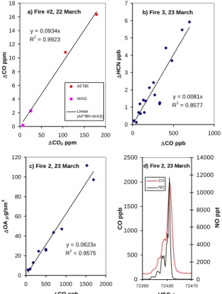
This method is justified in detail by Yokelson et al. (1999). When the AFTIR and the USFS WAS measured the same pair of compounds on the same fire, their data were combined in the plots as shown in Fig. 1a.

Emission ratios can also be obtained from the continuous instruments by comparing the integrals of ∆X and ∆Y as the aircraft passes through a nascent smoke plume.

25

(11)

ACPD

9, 767–836, 2009

the Yucatan

R. Yokelson et al.

Title Page

Tables Figures

◭ ◮

Back Close

Full Screen / Esc

through the plume of a single fire with continuous instruments (e.g. PM and CO₂on the Twin Otter), we plot the integrals versus each other and obtain the ER from the slope; analogous to grab sample plots. For the C-130 we usually compared integrals for vari-ous species to the integrals for CO. The exception was the PTR-MS. For the PTR-MS we obtained ER to methanol averaged over the three C-130 fires by comparing the

5

integrated excess for all 3 fires to the integrated excess amount for methanol. Finally, it is sometimes possible to use a “proxy” to generate continuous data from discrete samples. For example, the ratio of HCN to NOyshould not vary much throughout an

in-dividual plume. Thus, an estimate of the real-time variation in HCN can be obtained by multiplying the continuous NO_y data by the HCN/NO_y ratio measured intermittently in

10

the plume. Subsequently, the “continuous” HCN trace can be integrated and compared to integrals from other continuous instruments such as CO. For two species measured discretely by the Caltech CIMS (SO2and HCN) it was possible to compare the

“integral-based” ER to CO to the “plot-“integral-based” ER to CO. Compared to the integral-based ER, the plot-based approach returned individual fire ER that were identical when a few

15

minutes were spent in plume and up to 57% different for brief sample periods with an average di_fference of±21%. It is important to note, however, that the ER obtained from

the plot-based method did not show significant bias when averaged over several fires. Specifically, the plot-based ER was within 7% of the integral based ER averaged over 2 fires for SO₂, and within 5% averaged over 3 fires for HCN. We take this as a rough

20

estimate of the additional uncertainty affecting the study-average ER calculated from discrete samples. The lack of bias makes sense since e.g. a slower-responding CO instrument could read a little low when entering the plume, but a little high when leaving the plume. Figure 1 illustrates typical analyte levels encountered and gives examples of ER derivations.

25

It is also possible to estimate ER from measurements that were not made simulta-neously, or that were made on different aircraft. For example, the molar ER to CO2for

(12)

ACPD

9, 767–836, 2009

the Yucatan

R. Yokelson et al.

Title Page

Tables Figures

◭ ◮

Back Close

Full Screen / Esc

∆CO/∆CO2 ER measured on that same fire by AFTIR. The study-average molar ER

to CO2 for species measured on the C-130 (no CO2 data on C-130) was estimated

by multiplying the C-130 molar emission ratio to CO or CH₃OH by the study-average molar emission ratio of these latter species to CO2measured by AFTIR/WAS on board

the Twin Otter (on different fires). CO was measured with high accuracy by AFTIR, the

5

VUV instrument, and WAS. Methanol was measured with high accuracy by the AFTIR and PTR-MS. This facilitated coupling data from various platforms and instruments or for different fires. As a plume ages, the downwind NEMR (∆X/∆Y) can vary from the ER that was measured at the source. The accuracy of downwind∆X/∆Y may be re-duced by di_fferences in the time response of instruments, but in the dilute plume, the

10

excess mixing ratios tend to vary slower in time and space making timing differences less critical. Section 3.4 discusses uncertainty in the aging plume in detail.

2.4.1 Estimation of fire-average initial emission factors

For any carbonaceous fuel, a set of ER to CO2 for the other major carbon emissions

(i.e. CO, CH₄, a suite of non-methane organic compounds (NMOC), particle carbon,

15

etc) can be used to calculate emission factors (EF, g compound emitted/kg dry fuel burned) for all the emissions quantified from the source using the carbon mass-balance method (Yokelson et al., 1996). In this project, EF were calculated for all the individual fires sampled by the Twin Otter from AFTIR measurements of CO2, CO, CH4, and

NMOC and WAS measurements of CO2, CO, CH4, and non-methane hydrocarbons 20

(NMHC, a subset of NMOC consisting of compounds containing only C and H and no O or N). The nephelometer PM2.5and the AMS/PSAP measurements of the mass fraction

of C in the Yucatan BB aerosol (0.48±0.08) were used to estimate the particulate carbon. We also calculated study-average EF for the species measured on the C-130 by using the study average ER for those species to CO2 calculated using the overlap 25

species with the AFTIR as described above.

(13)

ACPD

9, 767–836, 2009

the Yucatan

R. Yokelson et al.

Title Page

Tables Figures

◭ ◮

Back Close

Full Screen / Esc

(Andreae and Merlet, 2001). We also assumed all the fires burned in fuels that were 50% C by mass on a dry weight basis (Susott et al., 1996), but the actual fuel carbon percentage could vary by±10% (2σ) of our nominal value. EF scale linearly with the assumed fuel carbon fraction. Because much of the NO is quickly converted to NO2

after emission, we also report an EF for “NO_xas NO.” For any species “X” we abbreviate

5

the EF as EFX.

2.5 Details of flights

2.5.1 Twin Otter flight of 12 March

Figure 2a shows the Twin Otter flight path over the Yucatan peninsula on 12 March along with the location of the fires that we sampled and the hotspots detected by

10

MODIS. (The MODIS hotspots were obtained from the Mexican Comisi ´on Nacional para el Conocimiento y Uso de la Biodiversidad (CONABIO) website at: http://www. conabio.gob.mx/conocimiento/puntos calor/doctos/puntos calor.html hereinafter cited as “CONABIO”). The fire locations and characteristics and any matches with hotspot lo-cations are also shown in Table 1. Widespread cloud cover over the Yucatan could have

15

obscured some fires during both of the satellite overpasses that covered the Yucatan: 10:34 LT (Terra 1, usually before most burning) and 13:38 LT (Aqua 2) (CONABIO). All 3 fires were sampled between 14:00 and 16:00 LT and all the fires were located near the coast S of Campeche. The fuel for all these fires was crop residue (CR) with a mi-nor fraction in adjoining woodlands on Fire #5. The fire numbers begin with #3 because

20

two fires were sampled enroute to the Yucatan that will be described elsewhere.

Figure 2b shows the Twin Otter flight path over the Yucatan peninsula on 22 March along with the locations of the fires sampled and the MODIS hotspots. The fire loca-tions, characteristics, and hotspot matches are also shown in Table 1. Eight fires were

(14)

ACPD

9, 767–836, 2009

the Yucatan

R. Yokelson et al.

Title Page

Tables Figures

◭ ◮

Back Close

Full Screen / Esc

sampled between 13:14 and 15:29 LT of which 5 were deforestation fires (DF, burning forest slash), and 3 were “mixed” (CR fires that escaped and burned adjacent forest, or CR/DF). (Sect. 4 gives more detail on the fires.) The sampling was all after the last satellite overpass with coverage of the Yucatan (Aqua 1 12:40 LT). At the time we sam-pled Fire #3 it was burning slash in a small clearing surrounded by intact forest. The

5

fire evidently began burning the adjacent forest by 23 March and was then sampled by the C-130 (see next section). Our Fire #8 was located near the coast in a patchwork of small fields and di_fferent-aged forests suggesting intensive use by small holders. The fire started as a crop residue fire, but spread to adjoining fields and forest. Strong surface winds pushed this fire aggressively towards the southeast. At 600–700 m

al-10

titude, the plume “curled back” and dispersed northwest at higher elevations. Three samples of this fire’s plume were obtained below 669 m (m.s.l.) and then 2 more were acquired at ∼1700 m where the plume had probably aged ∼10−30 min. Fire #8 was one of several sampled fires that were detected by MODIS and in the case of Fire #8 this indicates that it had burned for at least∼3 h.

15

2.5.3 C-130 flight of 23 March: Yucatan portion

On 23 March, from 14:05:35–14:06:39 LT, the C-130 descended through 3 closely spaced “stacked” smoke layers (with embedded fair-weather cumulus) near the top of the boundary layer (2200–2500 m) over the Yucatan (Fig. 2c; Table 1). The 3 high smoke layers had aged up to several hours and probably experienced some cloud

pro-20

cessing (based on the proximity of the clouds and the fact that the RH exceeded 100% as the C-130 passed through the middle layer). Next, at lower altitude, nascent smoke was sampled from 3 fires in the area; once per fire (14:09:31–14:16:47 LT). The sample of Fire #2 acquired by the C-130 on 23 March was located ∼750 m from the sample

acquired by the Twin Otter on 22 March of their “Fire #3.” A photograph of the C-130

25

(15)

ACPD

9, 767–836, 2009

the Yucatan

R. Yokelson et al.

Title Page

Tables Figures

◭ ◮

Back Close

Full Screen / Esc

The last C-130 sample of nascent smoke (from Fire #3 on 23 March) was at 1700 m and thus about 10–30 min old. Immediately after this sample, the aircraft stayed in the plume and followed the smoke in a curving path for about 14 km down wind probing smoke that had presumably aged an additional ∼1.5±0.7 h relative to the sample of

nascent smoke (14:16:48–14:18:31 LT) (Sect. 3.4). During the nominal aging interval

5

from 1.27–1.47 h the RH exceeded 100% indicating possible cloud processing. By 14:19:41 LT, the C-130 had climbed back above the boundary layer and set course for Veracruz.

Figure 2d shows the Twin Otter flight path over the Yucatan peninsula on 29 March,

10

the fires sampled (from 13:37–14:41 LT), and the hotspot locations (from Terra 1 at 11:16 LT and Aqua 1 at 12:46 LT). The fire, fire type, and hotspot matches are also in Table 1. In contrast to the 22 March flight when most of the fires found were DF, on 29 March all but one of the fires found were originally CR. Thus, of the six fires found, there was one DF, 3 CR, and 2 mixed (CR that escaped and also burned some woodland).

15

3 Results and discussion

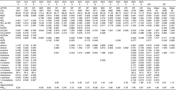
3.1 Fire-average initial emission factors measured on the Twin Otter

The fire-average emission factors (EF g/kg) measured on the Twin Otter are shown in Table 2 along with the study average EF for DF and CR fires. If molar ER are preferred for an application, they can be obtained from the EF in Table 2 with

consider-20

ation of the difference in molecular mass. The modified combustion efficiency – MCE,

(16)

ACPD

9, 767–836, 2009

the Yucatan

R. Yokelson et al.

Title Page

Tables Figures

◭ ◮

Back Close

Full Screen / Esc

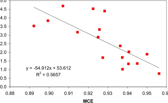
MCE and demonstrates that much of the large variation in EFCH₃OH (factor of ∼4.5)

is correlated with the different MCE that occur naturally on biomass fires. In princi-ple, it would be advantageous to incorporate this variability into emissions estimates. Unfortunately, at this time, MCE cannot be measured from satellites nor can seasonal trends in MCE be confidently assigned (Yokelson et al., 2008). For N and S species

5

EF variability also arises from the variable N and S components of the fuel (Yokelson et al., 1996, 2003, 2008). We note that the sum of the EF for gas-phase non-methane organic compounds (NMOC) in Table 2 is 12.8 and 12.0 g/kg for CR and DF fires, respectively. However, oxygenated volatile organic compounds (OVOC) normally dom-inate the gas-phase NMOC emitted by biomass fires and in this study many OVOC

10

common in biomass smoke were not measured on the Twin Otter. In an earlier study of fire emissions with enhanced detection of gas-phase OVOC, the combined instru-mentation could not identify about 50% of the gas-phase NMOC by mass (Yokelson et al., 2008). Therefore, we speculate that 30 g/kg is a conservative estimate of the real sum of gas-phase NMOC from these Yucatan fire types (see also Sect. 3.2).

15

3.1.1 Comparison to previous work on Yucatan and other deforestation fires

Cofer et al. (1993) made the only other fire emissions measurements in the Yucatan. They measured CO₂, CO, H₂, CH₄, and total NMHC (TNMHC) on two deforestation fires in February of 1990 and 1991. Utilizing all 23 WAS smoke samples and 11 back-grounds that they collected, yielded an average CO/CO2ratio of 0.071 – equivalent to 20

an MCE of 0.934. Their MCE is a little higher than our DF average (0.927), but well within our range for DF (0.907–0.945). We can not derive EF from their data because the average molecular mass and carbon fraction of their TNMHC is unknown. We can directly compare to their molar ratios to CO for H₂; 0.35±0.13; 0.44±0.21 (Twin Otter)

and CH4; 0.096±0.03; 0.125±0.056 (Twin Otter). Thus, while there is no statistically 25

(17)

ACPD

9, 767–836, 2009

the Yucatan

R. Yokelson et al.

Title Page

Tables Figures

◭ ◮

Back Close

Full Screen / Esc

above (and Sect. 3.2) that the Twin Otter total NMOC is too low. The present study does, however, greatly expand the extent of speciation of Yucatan fire emissions.

We compare our DF data to the most recent and extensive measurements of DF in the Amazon, a study which included both airborne measurements of nascent emissions and ground-based measurements of the smoldering emissions that cannot be sampled

5

from an aircraft (Yokelson et al., 2008). A few main features stand out. The largest difference occurs for initial emissions of particles. The EFPM₂_.₅ for the Twin Otter Yucatan DF is only 4.5±1.6 g/kg compared to 14.8±3.4 g/kg for the Amazon. Both of these values are significantly different from the recommendation of Andrea and Merlet (2001) of 9.1±1.5 g/kg, although their recommendation agrees remarkably well with 10

the average of the Yucatan and Amazon values (9.7 g/kg). A main factor contributing to the observed difference in EFPM2.5is probably that the March 2006 early dry season

fires that we were able to sample in the Yucatan were much smaller and less “intense” than the late dry season fires sampled in Brazil. As discussed in detail by Yokelson et al. (2007b) and references therein, it is likely that larger more intense fires have

15

much larger particle emission factors. Since a large fraction of annual biomass burning occurs late in the dry season, the late dry season EFPM may better represent the annual particle production. Also, we show in Sect. 3.4 that the ∆PM2.5/∆CO ratio

could increase by a factor of∼2.6 in∼1.4 h after emission. This factor times our initial

EFPM₂_.₅of 4.5 g/kg suggests that shortly after emission, about 12 g/kg of PM₂_.₅have

20

been produced even by the small Yucatan fires considered here.

The Yucatan fires had higher mean EFCO2; 1656±38 (1601 Amazon) and lower

mean EFCO; 83±14 (108 Amazon). This is indicative of relatively more flaming

com-bustion, which is also reflected in the higher MCE; 0.927 (0.904 Amazon). The higher MCE and a possible tendency for the biomass to be higher in nitrogen content may

ex-25

plain the higher mean EFNO_x; 4.7 (1.7 Amazon). Propene was also emitted in higher amounts from Yucatan fires; 1.36 (0.5 Amazon).

(18)

ACPD

9, 767–836, 2009

the Yucatan

R. Yokelson et al.

Title Page

Tables Figures

◭ ◮

Back Close

Full Screen / Esc

g/kg) for these compounds are: CH4(5.9 Yucatan, 6.3 Amazon); HCHO (2.6 Yucatan,

1.7 Amazon); CH3OH (2.98 Yucatan, 2.95 Amazon); NH3(.78 Yucatan, 1.1 Amazon);

ethane (1.08 Yucatan, 1.01 Amazon); ethene (1.05 Yucatan, 0.98 Amazon) and HCN (0.23 Yucatan, 0.66±0.56 Amazon). Two compounds had significantly lower emis-sions from the Yucatan deforestation fires: CH3COOH (2.9 Yucatan, 4.3 Amazon) and 5

HCOOH (below detection limit in Yucatan, 0.57 Amazon).

The EF measured for a single understory fire in a tropical dry forest in Africa were all within the range of EF we measured for the Yucatan DF, except that the EF for total PM for the African understory fire was 13 g/kg (Sinha et al., 2004). There are not enough measurements of understory fires to determine if their EF are significantly

10

different from the EF for DF. For species not measured in this study, the EF measured for deforestation fires in Brazil are probably the best estimate for these, and global tropical forest fires (Yokelson et al., 2008). By extension, the EF values measured in this work, but not in Brazil (Sect. 3.2) are likely the best estimate for global tropical forest fires.

15

3.1.2 Comparison of Yucatan deforestation and crop residue fires

We also compare the EF from the two main types of fires we observed in the Yucatan. Despite the fuel differences, the EF overlap within one standard deviation for most species. However, the tendency towards higher emissions of organic acids and am-monia from crop residue fires is clear; CH3COOH (4.8 CR, 2.9 DF); HCOOH (2.7 CR, 20

below detection limit DF); and NH₃ (1.38 CR, 0.775 DF). “Higher than normal” emis-sions of these species were also observed from burning rice straw by Christian et al. (2003) in a lab study.

The Yucatan DF emitted more HCHO than the CR fires we sampled (below detection limit CR, 2.6 DF). However, the rice straw fire sampled by Christian et al. (2003) had

25

(19)

ACPD

9, 767–836, 2009

the Yucatan

R. Yokelson et al.

Title Page

Tables Figures

◭ ◮

Back Close

Full Screen / Esc

may not be very sensitive to a shift in the relative amount of these two main fire types for most species.

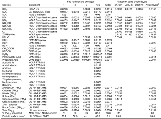
3.2 Fire initial emissions measured on the C-130

No CO2data was collected on the C-130 so we present ER to CO in Table 3. Also the

fuels were not positively identified so the C-130 data was not included in the “fire-type

5

specific” comparison above. However, the extensive instrumentation on the C-130, and the well-designed flight path, provided a large amount of valuable data.

The initial fire emissions of several species were measured for the first time in the field by the Caltech CIMS. These include H₂O₂, peroxyacetic acid, and propanoic acid. All these reactive compounds were present in significant amounts in the youngest

10

smoke samples. The presence of the peroxide species in the nascent smoke may reflect some fast initial photochemistry (e.g. recombination of peroxy radicals (RO₂, HO2)), but there is no increase in the peroxide species with altitude in our samples.

They are important as a HOx reservoir and the H2O2 plays an important role (along

with HCHO) in the oxidation of sulfur in clouds (Finlayson-Pitts and Pitts, 2000).

15

The NCAR SICIMS detected traces of H2SO4(∆H2SO4/∆CO, 5.4×10 −7

±5.2×10−7) and MSA (∆MSA/∆CO∼8.4×10−8±1.3×10−7) in the young fire emissions also for the first time. The initial amount of these species varies greatly probably due to variations in fuel S and plume reactivity.

The combination of PTR-MS and the Caltech CIMS made it possible to detect many

20

gas-phase NMOC that have been measured from fires before, but not on the Twin Otter in this study. In Table 4 where the results from the two aircraft are combined (as detailed in Sect. 3.3) the sum of identified gas-phase NMOC is 22 g/kg. This value is close to the sum of identified gas-phase NMOC for Brazilian deforestation fires (25.8 g/kg) reported by Yokelson et al. (2008). However, both of these values are only∼50% of the

25

(20)

ACPD

9, 767–836, 2009

the Yucatan

R. Yokelson et al.

Title Page

Tables Figures

◭ ◮

Back Close

Full Screen / Esc

of the molar ER to CO for measurable NMHC was 0.0393. Thus, the OVOC/NMHC ratio in the initial gas-phase emissions was about 3.3 – or OVOC accounted for 77% of measured, emitted NMOC on a molar basis. The dominance of NMOC by OVOC in BB plumes causes significant photochemistry differences compared to fossil fuel burning plumes, where NMOC are dominated by NMHC (Singh et al 1995; Mason et al., 2001).

5

An important species detected by PTR-MS was acetonitrile, which is thought to be produced almost exclusively by biomass burning (de Gouw et al., 2003) and thus has value as a BB tracer with relatively long (few months) atmospheric lifetime. The ER to CO for this species averaged over the 3 C-130 fires was 0.0043. The recommended acetonitrile to CO ER for 18 Brazilian DF was 0.0026±0.0007 (Yokelson et al., 2008). 10

Without better information on the variability of this ratio in the Yucatan we cannot say it is different from the ER for Brazilian DF. HCN is another compound produced mainly by biomass burning and used as a tracer (Li et al., 2000). The_∆HCN/∆CO ER measured on the C-130 was 0.0108±0.008 (n=3) and the Twin Otter ∆HCN/∆CO ER for all fires was 0.0032±0.0016 (n=17). The combined average for both aircraft is about

15

0.007±0.006, which is not significantly higher than the _∆HCN/_∆CO ER obtained for

Brazilian DF (0.0063±0.0054). The∆CH3CN/∆HCN molar ER is fairly consistent for

several recent field studies: 0.39 MC-area (J. Crounse private communication), 0.41 Brazil DF (Yokelson et al., 2008) and∼0.26 in the Yucatan if we only consider the fires

where both species were measured. The ∆CH3CN/∆HCN molar ER for laboratory 20

fires in six different tropical fuels was 0.56±0.31 (Christian et al., 2003).

As noted in Sect. 3.1.1, the Yucatan DF emitted more NO_x than Brazilian DF, which could suggest a higher fuel N content in the Yucatan and the hypothesis that NOx is

produced by oxidation of most of the N-containing compounds in the fuel. The fact that HCN and acetonitrile emissions are highly variable in both locations, but not larger

25

(21)

ACPD

9, 767–836, 2009

the Yucatan

R. Yokelson et al.

Title Page

Tables Figures

◭ ◮

Back Close

Full Screen / Esc

observations (Yokelson et al., 2008).

Both the Caltech CIMS and NOAA UV instruments confirmed higher than average emission of SO2from these fires. The average SO2/CO ER from the CIMS instrument

reflects one more fire than sampled by the NOAA UV instrument. The CIMS average molar ER of 0.0173 is approximately 7 times larger than the average for tropical forest

5

fires (0.0024) quoted by Andreae and Merlet (2001). The reason for this could involve the fuel S content, which could be high in the Yucatan because of soil S; manure used as fertilizer; or deposition of marine sulfur. There are some very large SO₂sources in central Mexico including volcanoes and petrochemical refineries (de Foy et al., 2007; Grutter et al., 2008). These sources are normally downwind of the Yucatan, but there

10

may be occasional meteorological circumstances where they contribute to sulfate de-position in the Yucatan.

The mean PM2.5 mass ratio to CO (0.0684±0.0054, Table 3) obtained by coupling

the UH nephelometer with the NCAR CO for the 3 C-130 fires was very similar to the average ratio obtained for all 17 fires on the Twin Otter (0.073±0.026). This suggests

15

that the two aircraft sampled a similar mix of biomass burning and confirms that the PM emissions were below the literature average for tropical forest fires. The UH PSAP allowed a rough measurement of black carbon (BC) based on light absorption. Martins et al. (1998) compared BC measurements by light absorption to those made by thermal evolution techniques. They found significant variation in the MAE with mixing state, size

20

distribution etc, and obtained an average MAE for fresh-aged Brazilian BB smoke of 12±4 m2/g. Using this MAE we obtained an average initial mass fraction of BC to PM₂_.₅ of 0.095±0.036, which is a little higher than the average initial mass fraction

obtained for Brazilian fires by Ferek et al. (1998) (0.071±0.012). Black carbon is the main component of smoke that lowers the single scattering albedo (SSA). Christian et

25

(22)

ACPD

9, 767–836, 2009

the Yucatan

R. Yokelson et al.

Title Page

Tables Figures

◭ ◮

Back Close

Full Screen / Esc

due to vigorous flaming, while Fire #2 had a lower buoyancy plume (C-130 flight video, http://data.eol.ucar.edu/). The plume dynamics are consistent with the BC and SSA data as Fires 1 and 3 had low SSA (0.67 and 0.73) and high BC/CO mass ratios (0.066 and 0.081) compared to Fire 2 (SSA 0.84, BC/CO 0.043).

From the OPC data, assuming spherical particles, we calculated the dry surface area

5

of particles 0.15–3 microns in diameter, which should account for most of the particle surface emitted (Table 3). The average value was 48±6.1 m2/g PM₂_.₅. The lowest

individual value was obtained for Fire #3 (41.1 m2/g PM2.5), which was sampled at the

highest altitude (1700 m) and likely reflected fast initial coagulation. The more aged upper haze layers had values near 30 m2/g PM₂_.₅, and this is likely a good estimate

10

of the dry surface area after most of the coagulation is complete. Ambient RH in the upper boundary layer ranged from 70–100% so the ambient particles would have been significantly larger due to addition of water. Measurements of the growth of BB parti-cles as they hydrate typically show an exponential increase in total scattering to about a factor of 2 near 80% RH, which is usually the cut-offfor the measurement (Magi and

15

Hobbs, 2003). Thus, the particle surface area could certainly double as “dry smoke” becomes “wet smoke.” Assuming an aged smoke layer dry PM2.5 of 100 µg/s m

3

we obtain a dry particle surface area concentration of ∼3×10−3m2/s m3. Multiplying by a typical number of active sites per m2 (1019, Bertram et al., 2001) suggests a “few ppbv” of active surface sites are available for heterogeneous chemistry in a typical wet

20

or dry smoke plume. This is a significant available surface area, but much smaller than the droplet surface area within clouds (up to 0.5 m2/s m3). The tendency of smoke-impacted clouds to have more, but smaller droplets (Kaufman and Nakajima, 1993) can cause the surface area in smoky clouds to be 2–7 times larger than in clean clouds. Depending on the extent of smoke-cloud interaction this could be the most important

25

influence of BB on available surface area.

(23)

ACPD

9, 767–836, 2009

the Yucatan

R. Yokelson et al.

Title Page

Tables Figures

◭ ◮

Back Close

Full Screen / Esc

mass fraction of each AMS species to the total PM₂_.₅ (Tables 3–5). These ratios can be compared to measurements in plume penetrations of nascent smoke from Brazilian fires by Ferek et al. (1998). (Since these ratios change rapidly after emission, it is best to compare initial ratios from similarly aged, very fresh samples.) Since Ferek et al., report a higher average ratio of PM4 to CO (0.10) this could bias a comparison of ratios

5

to CO between the two studies. Thus we compare our mass fractions of total PM2.5

to the mass fractions of total PM₄ that they obtained for the average of four fire types shown in their Table 3. The average MCE for their data treated in this manner is 0.924; close to the average MCE (0.929) measured on the Twin Otter for all Yucatan biomass burning.

10

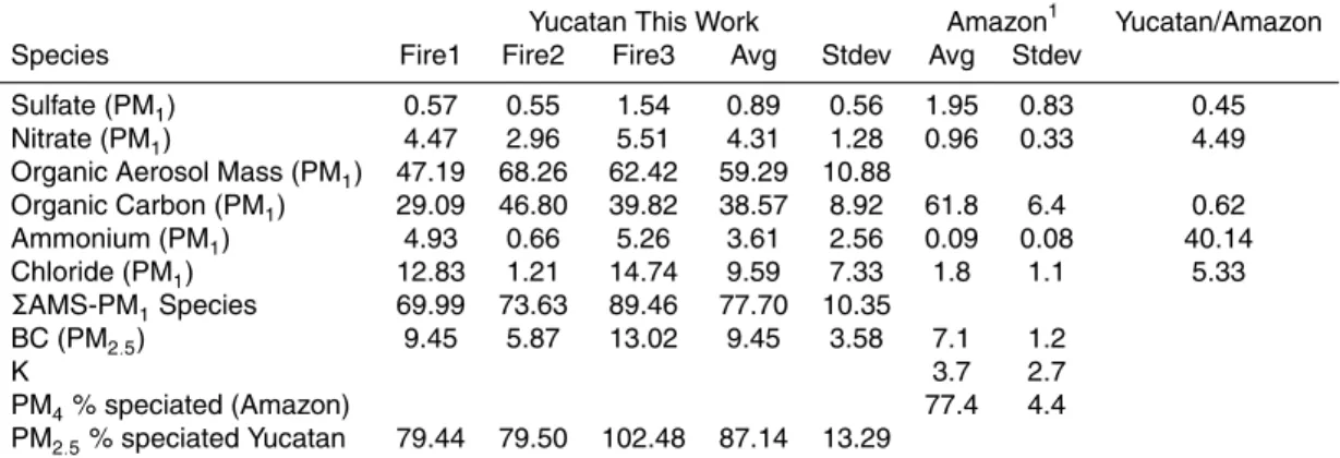
Fire #2, which may have been a forest fire (based on the video and photos) had the highest OA and lowest BC and is the C-130 fire that is most like the Brazil fires (Table 5). Fires 1 and 3 have much higher initial NR chloride, nitrate, and ammonium than Fire 2 or the Brazilian fires. This could indicate that these fires were burning crop residue and that the emissions were impacted by fertilizers. However, the high average EFCl− in

15

the Yucatan could also reflect wet deposition of marine aerosol on the fuels (McKenzie et al., 1996). The lower EFCl− for Fire #2 might indicate that it was not burning hot enough to volatilize the fuel chlorine efficiently. Despite the high SO2emissions from

the Yucatan fires the initial PM2.5 is not elevated in sulfate, which makes sense since

the atmospheric oxidation of SO₂to sulfate typically requires about a week. The sum of

20

species characterized by Ferek et al. on their filters was about 77% of their PM4. The

main species they did not measure is non-carbon organic mass since they analyzed for organic carbon (OC) only. Adding their residue to their OC suggests a_∆OA/∆OC ratio of∼1.34±0.11, which is a little lower than the∆OA/∆OC of 1.55±0.08 measured by the AMS for the Yucatan fires. The average Yucatan OC was 39±9% of the PM2.5 25

on a mass basis, which is below the average of∼62±6% obtained by Ferek et al. in

(24)

ACPD

9, 767–836, 2009

the Yucatan

R. Yokelson et al.

Title Page

Tables Figures

◭ ◮

Back Close

Full Screen / Esc

“refractory” in other studies may be detected by the AMS. Finally, one African tropical dry forest fire emitted “total” PM that was only 23% OC (Sinha et al., 2004). The sum of the species analyzed on the C-130 accounted for 87±13% of the total PM2.5 as

calculated from our MSE-based approach. Other methods of computing total PM₂_.₅on the C-130 could be used such as the size distribution coupled with the particle number

5

and an assumed density. But the agreement obtained from the MSE-based approach is adequate as each technique only claims accuracy of∼25%. The main aerosol species

not quantified on the C-130 is potassium (K). The K+ signal in the AMS can reflect both surface and electron impact ionization making it difficult to quantify the amount of K in ambient particles. K was about 3.7% of particle mass in Ferek et al., but

10

its incorporation into particles depends strongly on the amount of flaming combustion (Ward and Hardy et al., 1991) as may also be the case for chloride.

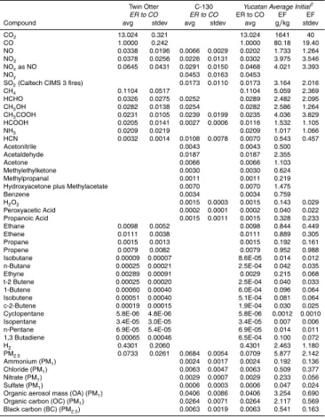
3.3 Overall combined initial emissions from Yucatan biomass burning

In this study we simply take the average of all the Twin Otter data and weight it equally to the average of all the C-130 data. As discussed in Sect. 4, this approach may weight

15

the emissions from CR fires too heavily to be a true regional average, but it allows us to use the valid measurements from mixed or unknown fire types. Since, we have also presented the emissions data in the original stratified form (Tables 2 and 3), this allows alternate coupling schemes for future applications. In any case, as noted above, the fire type may not affect the smoke chemistry dramatically except for organic acids, NH3, 20

and some PM species. In addition, the smoke transported away from the Yucatan will not have the same composition as the initial emissions due to rapid photochemistry detailed in Sect. 3.4.

To couple data from both aircraft in our estimate we proceed as follows. Both molar ER to CO and EF are useful for regional estimates and only the former was measured

25

(25)

ACPD

9, 767–836, 2009

the Yucatan

R. Yokelson et al.

Title Page

Tables Figures

◭ ◮

Back Close

Full Screen / Esc

fires sampled by the C-130. In Column 6 the combined average ER to CO is shown for all species. When a species was measured on both aircraft or by two instruments we took the straight average of the two values as our preliminary estimate of the study average regional value (except for SO₂ as detailed above). Finally, in Column 7, the study-average initial ER from Column 6 have been converted to EF using the Twin Otter

5

average CO/CO2and the carbon mass balance method (Sect. 2.4.1).

It is worth noting briefly that, on average, similar fires were sampled by each aircraft. The PM2.5/CO ratios are close as noted above. A best calculation of the methanol

to CO ratio measured on the C-130 (allowing for sampling rate differences) gives an average value for the three C-130 fires of 0.0254, which is within 10% of the

aver-10

age measured by AFTIR for the 17 fires sampled on the Twin Otter (0.0282). The

∆CH3COOH/∆CO and∆HCHO/∆CO ER measured on the two different aircraft were

also very similar (Table 4). The means were not as close for NOx and HCN, but the

standard deviation about the mean was large for both species on both aircraft. We do note that, the∆HCN/∆CO ER measured on Fire #3 by the AFTIR on 22 March was

15

0.0037, which is not far from the value measured by the Caltech CIMS (0.0047) on the continuation of that fire the next day, though perhaps burning partly di_fferent fuels.

3.4 Photochemical aging of smoke (first 1.5 h)

Post-emission chemistry determines much of the atmospheric impact of smoke from fires. In this study, the C-130 first sampled Fire #3 at 1700 m where the smoke

20

would have been ∼10−30 min old and then immediately followed the plume

down-wind. About 14 km downwind,∆CO in the plume suddenly decreased from values that were≥10−20 times the variation in the background (∼5 ppbv CO) to only 2–3 times the

background variation. The measurements continued beyond this point, but we do not discuss them since the excess values are highly uncertain. The average windspeed

25

measured in the aging plume was 9.6±4.2 km/h. Assuming the average winds were

(26)

ACPD

9, 767–836, 2009

the Yucatan

R. Yokelson et al.

Title Page

Tables Figures

◭ ◮

Back Close

Full Screen / Esc

In Fig. 4a,∆O3/∆CO is plotted versus the estimated change in smoke age. A rapid

increase in this ratio to∼15% occurs in<1 h. Figure 4a also shows∆Ox/∆CO versus

time where “O_x” approximates the total odd oxygen. In this work the sum of O₃, NO₂, and PANs account for nearly all the odd oxygen. The rise in∆Ox/∆CO is very

simi-lar to that in ∆O3/∆CO confirming that O3 is being produced through photochemical 5

oxidation of NMOC (Crutzen et al., 1999). Yokelson et al. (2003) measured a rise in

∆O₃/∆CO to∼9% in∼0.7 h on 3 isolated BB plumes in Africa and the_∆O₃/_∆CO

ob-served in this work after∼0.7 h of smoke aging (∼8%) is close to the value observed in the African plumes. The chemical evolution of one of the above-mentioned African plumes was measured in great detail (Hobbs et al., 2003) and Trentmann et al. (2005)

10

constructed a comprehensive photochemical model for comparison with those mea-surements. The model agreed with the measured rate of increase in∆O3/∆CO only

if plausible, but unconfirmed, heterogeneous reactions were added; or if the measured initial emissions of NMOC were increased by 30% (on a molar basis) as a surrogate for unmeasured NMOC. The latter assumption is consistent with our earlier statement

15

that ∼50% of the NMOC emitted by BB are unidentified on a mass basis and this

should perhaps be a standard assumption in the modeling of BB plumes. The rate of increase in∆O3/∆CO seen in the Yucatan and Africa is faster than observed in some

BB plumes; especially at high latitudes (Goode et al., 2000; De Gouw et al., 2006), but most BB occurs in the tropics. In any case, from southern Africa to Alaska it has

20

been shown that large-scale chemical changes can occur in BB plumes in an initial photochemical regime that is different from the ambient boundary layer and at a spatial scale that could challenge regional-global models.

In Fig. 4a, and some of the figures that follow, there is some non-monotonic struc-ture and/or “scatter” in the downwind normalized excess mixing ratios (NEMR). This is

25

(27)

ACPD

9, 767–836, 2009

the Yucatan

R. Yokelson et al.

Title Page

Tables Figures

◭ ◮

Back Close

Full Screen / Esc

decay in total smoke concentration downwind. (2) The fuels and initial emissions can vary over the course of a fire. When a fire burns freely into homogeneous fuels, the flaming/smoldering ratio and the initial emission ratios may be fairly constant (Hobbs et al., 2003), but this is not always the case. (3) Mixing with fresh or aging plumes from other fires is possible. _∆HCN/∆CO is one of the ER that varies the most from fire to

5

fire and this NEMR was fairly constant for the 1.5 h of Fire #3 data we show. (Figure 1b shows all the HCN and CO values in the aging Fire #3 plume.) However, some degree of mixing with other plumes cannot be completely ruled out.

A rigorous error estimate is not possible for each of the above terms or the assump-tion of a similar windspeed before our sampling. Thus we point out obvious trends in

10

the data and, in some cases, we fit a line to the data and compare the slope to the standard error in the slope to determine if there is a statistically significant trend. The fractional uncertainty in the rate of any process discussed is larger than the standard error divided by the slope due to the additional uncertainty in the sample ages. Proba-bly all the samples have experienced more aging, or all the samples have experienced

15

less aging, than estimated. The real uncertainty in the rate is probably about a factor of two.

Figure 4b suggests that there were likely some gradual changes in the initial emis-sions of Fire #3 and the post-emission processing environment that help interpret our data in the aging plume. Figure 4b shows∆BC/∆CO at the 5 s time resolution of the

20

PSAP. BC is a flaming product and CO is a smoldering product. As the C-130 flew downwind in the plume, the gradual 20% decrease in∆BC/∆CO until about 0.9 h sug-gests the instruments were sampling smoke originally produced at a gradually decreas-ing flamdecreas-ing/smolderdecreas-ing (F/S) ratio. The peak in BC/CO at∼1 h could reflect a tempo-rary increase in the F/S ratio at the source about an hour before the sampling started.

25

For the older samples, the F/S ratio was again close to the F/S ratio at the time of the first C-130 sample. Thus a comparison of the beginning and end NEMRs may best re-flect post-emission chemistry. The variation in JNO₂ is also shown in Fig. 4b. JNO₂ first

(28)

ACPD

9, 767–836, 2009

the Yucatan

R. Yokelson et al.

Title Page

Tables Figures

◭ ◮

Back Close

Full Screen / Esc

JNO₂ decreases by∼2,∆O3/∆CO decreases slightly, and CO increases. The aircraft

is evidently entering a region of the plume with greater total smoke concentration. Af-ter one hour, both∆O₃/∆CO and J_NO

2 increase, the smoke concentration decreases,

and minimal cloud-processing may occur.

A key driver for photochemistry besides UV is OH. In Hobbs et al. (2003) the rate of

5

decrease of numerous NMHC in one African biomass burning plume was used to esti-mate an average plume OH over the first 40 min of aging of∼1.7×107molecules/cm3.

On our Fire #3, no NMHC were measured within the aging plume, but an OH instru-ment was on board. The first OH value in the aging plume (averaged over 29 s of flight time and a calculated range of smoke aging of 22–43 min) is 1.14×107molecules/cm3. 10

This is 5–20 times larger than the OH values in nearby background air. The plume OH levels thereafter decreased to about twice the average OH in the boundary layer. To our knowledge this is the first in-situ measurement of OH in a BB plume and it confirms the potential for very high initial OH in BB plumes. The measurements imply a major shortening of reactive species “lifetimes” in comparison to ambient air as predicted

ear-15

lier (Mason et al., 2001). HO₂and RO₂would likely be elevated along with OH (Mason et al., 2001). However, the one minute time resolution of the HO2instrument and some

missing data make it difficult to determine the levels of this species in the 3 BB plumes sampled on the C-130.

Trace gases other than O3also increased. The initial∆HCHO/∆CO from the NCAR 20

DFG spectrometer was 0.025±0.01 and it increased to 0.038±0.01 at 0.8±0.1 h. Sim-ilar increases in this NEMR were also seen in an African plume in samples acquired near the top of the plume (Hobbs et al., 2003). The∆HCHO/∆CO increased dramat-ically when smoke entered a cloud in Africa (Tabazadeh et al., 2004) and may have also increased strongly in the Fire 3 plume for the points that may be cloud impacted

25

(∼0.065±0.025).

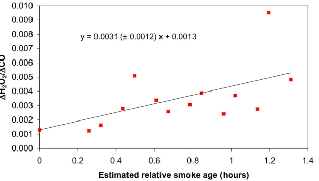
The ratio ∆H2O2/∆CO was 0.0013 in the nascent smoke from Fire #3 and then

increased by ∼4 to 0.0054 after ∼1.3 h of aging (Fig. 5). In Fig. 5, the intercept is

(29)

ACPD

9, 767–836, 2009

the Yucatan

R. Yokelson et al.

Title Page

Tables Figures

◭ ◮

Back Close

Full Screen / Esc

∆CO for all the samples in the nascent smoke of Fire #3. We force the intercept because it is based on more samples (with higher S:N) and it has lower uncertainty than the individual downwind NEMRS. With additional aging, the ∆H2O2/∆CO ratio

would likely increase significantly beyond the ratio measured at 1.3 h due to lower NO_x and entrainment of the BL air which had an absolute H2O2/CO ratio of 0.0125. Lee et 5

al. (1997) observed∆H2O2/∆CO ratios of 0.01–0.046 in BB-impacted SH BL air.

Figure 6 shows post-emission growth in peroxyacyl nitrates both as∆PAN/∆CO and

∆ΣPANs/∆NOy. An initial value for ∆PAN or ∆ΣPAN may not be meaningful (as for O3) and was not measured due to interference in the nascent smoke. However, Fig. 6a

shows that the∆PAN/∆CO ratio increases rapidly from∼0.0025 (at∼0.4 h) to∼0.006 10

(at∼1.4 h). The NEMR reached in∼1.4 h is as large as the NEMR observed in smoke

from Canada that was∼8 days old during NEAQS (F. Flocke private communication). This demonstrates the large variability in both initial emissions and photochemical rates that are associated with BB plumes. Figure 6b shows the_∆ΣPANs/∆NOy with aging in the Fire #3 plume. In the∼1.2−1.4 h aging interval,∆PAN/∆NOyalone has increased 15

to about 13%. The other PAN-like species showed similar trends, but were present in smaller amounts. The sum of the most abundant other PAN-like species (APAN and PPN) was about 20% of PAN in the 1.2–1.4 h interval and the∆ΣPANs/∆NOy had

in-creased to 0.167±0.036 in this interval. In the initial Fire #3 plume∆NO_x/∆NO_ywas

0.76 (based on comparing integrals) and in the 1.2–1.4 h aging interval∆NOx/∆NOy 20

was 0.41±0.1. This implies a NOx loss of 46±11%. A second estimate of the

percent-age of NO_x loss based on the decrease in_∆NO_x/∆CO is 62±16%. Averaging these

estimates of the NOx loss gives 54±19% implying that PANs accounted for 31±13%

of the loss of NOx. Similar trends were not observed for HNO3. Modestly elevated

mixing ratios of HNO₃occurred in some parts of the BL, but were not correlated with

25

the obvious presence of fresh or aged smoke (i.e. elevated CO). The NH3/NOxmolar