Stable atmospheric methane in the 2000s: key-role of emissions from natural wetlands

(1)

ACPD

13, 9017–9049, 2013

Stable atmospheric methane in the 2000s

I. Pison et al.

Title Page

Abstract Introduction

Conclusions References

Tables Figures

◭ ◮

Back Close

Full Screen / Esc

Printer-friendly Version Interactive Discussion

Discussion

P

a

per

|

Dis

cussion

P

a

per

|

Discussion

P

a

per

|

Discussio

n

P

a

per

|

Atmos. Chem. Phys. Discuss., 13, 9017–9049, 2013 www.atmos-chem-phys-discuss.net/13/9017/2013/ doi:10.5194/acpd-13-9017-2013

Atmospheric Chemistry and Physics

Open Access

Discussions

Geoscientific Geoscientific

This discussion paper is/has been under review for the journal Atmospheric Chemistry and Physics (ACP). Please refer to the corresponding final paper in ACP if available.

Stable atmospheric methane in the 2000s:

key-role of emissions from natural

wetlands

I. Pison1, B. Ringeval2,3,4, P. Bousquet1, C. Prigent5, and F. Papa6,7

1

Laboratoire des Sciences du Climat et de l’Environnement, Institut Pierre-Simon Laplace, CEA/CNRS/UVSQ, UMR8212, Gif-sur-Yvette, France

2

Institute of Marine and Atmospheric Research Utrecht, Utrecht University, Utrecht, the Netherlands

3

SRON Netherlands Institute for Space Research, Utrecht, the Netherlands

4

Vrije Universiteit, Department of Systems Ecology, Amsterdam, the Netherlands

5

Laboratoire d’ ´Etudes du Rayonnement et de la Mati `ere en Astrophysique, Observatoire de

Paris, CNRS, Paris, France

6

Laboratoire d’ Études en G éophysique et Oc éanographie Spatiales, Institut de Recherche

pour le D ´eveloppement, Toulouse, France

7

(2)

ACPD

13, 9017–9049, 2013

I. Pison et al.

Title Page

Tables Figures

◭ ◮

Back Close

Full Screen / Esc

Discussion

P

a

per

|

Dis

cussion

P

a

per

|

Discussion

P

a

per

|

Discussio

n

P

a

per

|

Received: 1 February 2013 – Accepted: 20 March 2013 – Published: 4 April 2013

Correspondence to: I. Pison (isabelle.pison@lsce.ipsl.fr)

(3)

ACPD

13, 9017–9049, 2013

I. Pison et al.

Title Page

Tables Figures

◭ ◮

Back Close

Full Screen / Esc

Discussion

P

a

per

|

Dis

cussion

P

a

per

|

Discussion

P

a

per

|

Discussio

n

P

a

per

|

Abstract

Two atmospheric inversions (one fine-resolved and one process-discriminating) and a process-based model for land surface exchanges are brought together to analyze the variations of methane emissions from 1990 to 2009. A focus is put on the role of natural wetlands and on the years 2000–2006, a period of stable atmospheric concentrations.

5

From 1990 to 2000, the two inversions agree on the time-phasing of global emis-sion anomalies. The process-discriminating inveremis-sion further indicates that wetlands dominate the time-variability of methane emissions with 90 % of the total variability. Top-down and bottom-up methods are qualitatively in good agreement regarding the global emission anomalies. The contribution of tropical wetlands on these anomalies is

10

found to be large, especially during the post-Pinatubo years (global negative anomalies with minima between₋41 and₋19 Tg y−1_{in 1992) and during the alternate 1997–1998}

el-Ni ˜no / 1998–1999 la-Ni ˜na (maximal anomalies in tropical regions between+16 and

+22 Tg y−1_{for the inversions and anomalies due to tropical wetlands between}

+12 and

+17 Tg y−1_{for the process-based model).}

15

Between 2000 and 2006, during the stagnation of methane concentrations in the atmosphere, total methane emissions found by the two inversions on the one hand and wetland emissions found by the process-discriminating-inversion and the pro-cess model on the other hand are not fully consistent. A regional analysis shows that di_fferences in the trend of tropical South American wetland emissions in the

20

Amazon region are mostly responsible for these discrepancies. A negative trend (−3.9±1.3 Tg y−1) is inferred by the process-discriminating inversion whereas a

pos-itive trend (₊1.3±0.3 Tg y−1) is found by the process model. Since a positive trend

is consistent with satellite-derived extent of inundated areas, this inconsistency points at the difficulty for atmospheric inversions using surface observations to properly

con-25

(4)

ACPD

13, 9017–9049, 2013

I. Pison et al.

Title Page

Tables Figures

◭ ◮

Back Close

Full Screen / Esc

Discussion

P

a

per

|

Dis

cussion

P

a

per

|

Discussion

P

a

per

|

Discussio

n

P

a

per

|

some inventories for the early 2000s, although process-based models have also their own caveats and may not take into account all processes.

1 Introduction

The growth rate of atmospheric methane (CH₄) has experienced large variations since the early 1990s: after a decade of decrease, interrupted by two peaks in 1997–1998

5

and 2002–2003 (Dlugokencky et al., 1998; Cunnold et al., 2002; Wang et al., 2004; Bousquet et al., 2006), the growth rate of atmospheric methane remained small from 1999 to 2006, only to increase again since 2007 (Rigby et al., 2008; Dlugokencky et al., 2009; Bousquet et al., 2011). As methane is emitted by a large variety of sources, the explanations for the observed atmospheric variations have generally implied changes

10

in several source or sink types.

The sources involved in the variations of the 1990s are now well understood, al-though their relative magnitude may still be debated.

The 1991–1993 growth rate anomaly is linked to the Pinatubo eruption, which led to a decrease in methane loss, due to reduced tropospheric hydroxyl radical (OH)

15

concentrations and stratospheric chemistry changes (B ˆand ˘a et al., 2012), followed by a decrease in natural wetland emissions. The negative impact of this volcanic event on wetland CH₄ emissions is due to its e_ffects on the climate, with both cooling (Dlugo-kencky et al., 1996) and precipitation anomalies in the Northern hemisphere (Walter et al., 2001b; Dlugokencky et al., 2011), likely slightly amplified by sulfur deposition

20

(Gauci et al., 2008). The collapse of the economy of the former USSR and Eastern Eu-rope has also led to decreased anthropogenic emissions starting in 1991 and spanning most of the 1990s (Dlugokencky et al., 2003).

The 1997–1999 large growth rate anomaly is explained by a positive anomaly in emissions from biomass burning, both in the Tropics and at high latitudes (van der

25

(5)

ACPD

13, 9017–9049, 2013

I. Pison et al.

Title Page

Tables Figures

◭ ◮

Back Close

Full Screen / Esc

Discussion

P

a

per

|

Dis

cussion

P

a

per

|

Discussion

P

a

per

|

Discussio

n

P

a

per

|

by a positive anomaly in the same in 98-99, linked to wet la-Ni ˜na conditions (Bousquet et al., 2006; Chen and Prinn, 2006).

Overall, the role of wetlands in changes in atmospheric methane has often been identified as dominant (Chen and Prinn, 2006; Bousquet et al., 2006, 2011), linked to meteorological conditions of temperatures and precipitations (Dlugokencky et al.,

5

2009; Bousquet et al., 2011). These conditions are thought to lead to changes in both the wetland extent (e.g. Ringeval et al., 2010) and the CH₄flux per wetland area (e.g. Bloom et al., 2010). The impact of wetland emissions is often thought to be combined with changes in OH concentrations (Wang et al., 2004; Monteil et al., 2011), although it is now well accepted that inter-annual changes in OH concentrations are limited to

10

1-3 % and can therefore explain only a limited part of the observed changes in the methane growth rate (Montzka et al., 2011).

The analysis of the variations of atmospheric methane after 1999 is still largely de-bated.

Various scenarios have been suggested to explain the stabilization of methane

con-15

centrations between 2000 and 2006: (i) reduced global fossil-fuel-related emissions, estimated from AGAGE and NOAA (Chen and Prinn, 2006) or from ethane emissions used as a proxy to fossil-fuel-related CH₄emissions (Aydin et al., 2011; Simpson et al., 2012); (ii) compensation between increasing anthropogenic emissions (as inferred by inventories such as EDGAR4 (EDGAR 4, 2009)) and decreasing wetland emissions

20

(Bousquet et al., 2006); (iii) a decrease in emissions due to rice-paddies, attributed to changes in agricultural practices (Kai et al., 2011); (iv) stable microbial and fossil-fuel-related emissions in the early 2000s (Levin et al., 2012) and/or (v) significant (Rigby et al., 2008) to small (Montzka et al., 2011) changes in OH concentrations.

The increase of methane concentrations observed since 2007 (Rigby et al., 2008;

25

(6)

ACPD

13, 9017–9049, 2013

I. Pison et al.

Title Page

Tables Figures

◭ ◮

Back Close

Full Screen / Esc

Discussion

P

a

per

|

Dis

cussion

P

a

per

|

Discussion

P

a

per

|

Discussio

n

P

a

per

|

Methane emissions can be investigated using process-based models and inventories (bottom-up or B-U approach), and atmospheric inversions (top-down or T-D approach). Atmospheric inversions combine atmospheric observations of CH₄, an atmospheric chemistry and transport model, and prior information about sources and sinks. The flux estimates that give the best fit to the observed atmospheric concentrations are

5

derived by optimization. However, atmospheric inversions provide a limited insight into the underlying biogeochemical processes controlling emissions, particularly over re-gions where several processes and sources overlap. B-U models computing wetland (Melton et al., 2012) or biomass-burning (van der Werf et al., 2010) methane emissions incorporate knowledge of small-scale processes but they need additional information

10

and constraints to project their local emission estimates to larger scales compatible with the atmospheric signals. B-U emission inventories (EDGAR 4, 2009; EPA, 2011) are based on country-scale energy use and agricultural statistics and usually provide yearly to decadal estimates of anthropogenic emissions at global and national scales.

In this study, we present an analysis of methane fluxes for the 1990–2009 period.

15

We specially investigate the relative contributions of the various emissions leading to the stable concentrations during the 2000–2006 period. For this, we bring together the T-D and B-U methodologies to analyze the variations of methane emissions and assess the particular role of emissions from natural wetlands. We study (i) the total methane emissions, as inferred by two different atmospheric inversions (T-D); (ii) the

20

wetland emissions, as inferred by one inversion (the one which is able to discriminate the various sources or sinks) and by one process-based model of vegetation (B-U). The methodology of the process-based model and the two inversions is described in Sect. 2; results are given in Sect. 3 at the global (Sect. 3.1) and regional (Sect. 3.2) scales.

(7)

ACPD

13, 9017–9049, 2013

I. Pison et al.

Title Page

Tables Figures

◭ ◮

Back Close

Full Screen / Esc

Discussion

P

a

per

|

Dis

cussion

P

a

per

|

Discussion

P

a

per

|

Discussio

n

P

a

per

|

2 Methodology

We combine the results of a process-based model for natural wetland emissions, OR-CHIDEE (Krinner et al., 2005; Ringeval et al., 2010, 2011), together with the CH₄fluxes estimated by two different atmospheric inversions, variational (Chevallier et al., 2005; Pison et al., 2009) and analytical (Bousquet et al., 2005).

5

2.1 Process model for natural wetland emissions

The model of CH₄emissions by natural wetlands used here (hereafter ORCHIDEE) is based on the ORCHIDEE global vegetation model (Krinner et al., 2005) which simu-lates land energy budget, hydrology, and carbon cycling. It has then been developed (Ringeval et al., 2010, 2011) to simulate:

10

– the CH₄-emitting wetland area dynamic, using some TOPMODEL concepts (Ringeval et al., 2012a). The wetland extents are here normalized to match Papa et al. (2010). A global, multi-year data set giving the monthly distribution of flooded areas at a≈25 km resolution has been generated. It is based on multiple satellite

observations which are optimized specifically for surface water detection (Papa

15

et al., 2010; Prigent et al., 2012). It is built using a combination of satellite data including passive microwave observations and a linear mixture model to account for vegetation. Three wetland classes, di_ffering by the value of the water table depth, are simulated for each grid cell and at each time step: saturated wetland and wetland with a mean water table at 3 and 9 cm below the soil surface.

20

– the flux density, which is computed following Walter et al. (2001a) and Ringeval et al. (2010) and results from three processes: production, oxidation and transport (via diffusion, ebullition and through plants).

A summary of the ORCHIDEE methodology used to compute CH₄emissions is given in Wania et al. (2012).

(8)

ACPD

13, 9017–9049, 2013

I. Pison et al.

Title Page

Tables Figures

◭ ◮

Back Close

Full Screen / Esc

Discussion

P

a

per

|

Dis

cussion

P

a

per

|

Discussion

P

a

per

|

Discussio

n

P

a

per

|

The wetland emissions are driven by the CRU-NCEP climate forcing data set (Viovy and Ciais, 2009). In this study, four scenarios of wetland emissions are given based on:

– accounting or not for the non-saturated wetlands (i.e. all classes of wetlands or saturated wetlands only)

5

– multiplying or not the simulated wetland area by peat-land map in boreal regions. This map is obtained by using soil organic carbon data from IGBP DIS at high resolution (5′×5′), by dividing each pixel of this database by 130 kg m−3 (which

is the maximum soil carbon density of peat), and then by regridding the result at 1◦

×1 ◦ resolution (Lawrence and Slater, 2007). The hypothesis underlying the

10

multiplication of the two products (map of peat-land cover and map of inundated areas) is that the inundated fraction is the same for an entire grid-cell as for a sub-grid peat-land into this sub-grid-cell (see Bousquet et al., 2011, for more details). ORCHIDEE provides CH₄ emissions by natural wetlands as the product of a flux density by a wetland extent, at a 1 degree by 1 degree resolution for the time period

15

1990–2009.

Note that ORCHIDEE emissions are not used as prior emissions in INVANA nor INVVAR (Sect. 2.2).

2.2 Inverse methods

The two inversion models used here are based on the Bayesian formalism: they

assim-20

ilate surface observations of CH₄and methyl-chloroform (CH₃CCl₃or MCF) concentra-tions (measurements from various surface monitoring networks: AGAGE (Prinn et al., 2000, accessed: 2012-03-31), CSIRO (Francey et al., 1999), EC (Worthy et al., 1998), ENEA (Artuso et al., 2007), AEMET (Gomez-Pelaez et al., 2010), JMA (Matsueda et al., 2004), LSCE (Schmidt et al., 2005), NIWA (Lowe et al., 1991), NOAA/ESRL

25

(9)

ACPD

13, 9017–9049, 2013

I. Pison et al.

Title Page

Tables Figures

◭ ◮

Back Close

Full Screen / Esc

Discussion

P

a

per

|

Dis

cussion

P

a

per

|

Discussion

P

a

per

|

Discussio

n

P

a

per

|

model (Hourdin et al., 2006) with prior information on the spatio-temporal distribution and uncertainties of CH₄sources and sinks to estimate the magnitude and the uncer-tainties of optimized surface emissions. The two methods di_ffer by the inversion setup and the resolution method: see Bousquet et al. (2005) and Pison et al. (2009).

The analytical scheme (hereafter INVANA) is described in more details in Bousquet

5

et al. (2005, 2011). Briefly, it solves for monthly emissions for various types of sources and sinks in ten land regions plus one global ocean. The constraints are monthly mean CH₄concentrations at 68 surface stations (CSIRO (Francey et al., 1999), LSCE (Schmidt et al., 2005), NOAA/ESRL (Dlugokencky et al., 1994, 2009)) with monthly uncertainties ranging from±5 ppb to ±50 ppb, with a median of ±10 ppb. The

trans-10

port model is LMDZt v3 o_ffline nudged on analyzed horizontal winds (Uppala et al., 2005; Hourdin et al., 2006) with OH pre-optimized using methyl-chloroform concen-trations (Bousquet et al. (2005) used MCF concentration measurements by AGAGE (Prinn et al., 2005) and NOAA/ESRL (Montzka et al., 2000, 2011)). The prior emis-sions are elaborated from various inventories by Matthews and Fung (1987), Olivier

15

and Berdowski (2001) and van der Werf et al. (2006). Monthly uncertainties on fluxes are set at 150 % in each region; there are no error correlations but month-to-month changes are limited to _±250 % if the process follows a seasonal cycle or to _±50 % otherwise (Peylin et al., 2000, 2002).

The main advantage of this inversion scheme is the low cost of computation, which

20

makes it possible to test various scenarios, varying OH concentrations, constraints, uncertainties. In this study, eleven scenarios are used, as described in Bousquet et al. (2011).

The variational scheme (hereafter INVVAR) is described in Chevallier et al. (2005) and Pison et al. (2009). Briefly, it solves for weekly net emissions at grid-point

reso-25

lution (2.5◦

×3.75◦). The constraints are daily mean observations at continuous

(10)

ACPD

13, 9017–9049, 2013

I. Pison et al.

Title Page

Tables Figures

◭ ◮

Back Close

Full Screen / Esc

Discussion

P

a

per

|

Dis

cussion

P

a

per

|

Discussion

P

a

per

|

Discussio

n

P

a

per

|

2010), JMA (Matsueda et al., 2004), LSCE (Schmidt et al., 2005), NIWA (Lowe et al., 1991), NOAA/ESRL (Montzka et al., 2000, 2011; Dlugokencky et al., 1994, 2009), SAWS (Brunke et al., 2001), UBA (UBA, 2013). All methane data were re-scaled to the NOAA 2004 methane standard scale (Dlugokencky et al., 2005). The differences in MCF scales have been included in the errors associated to MCF observation

er-5

ror statistics i.e. in the variances attributed to the differences between measured and simulated MCF concentrations. The chemistry-transport model is LMDZt v4 – SACS (Pison et al., 2009) with prior OH fields provided by a full-chemistry run with the INCA scheme (Hauglustaine et al., 2004; Folberth et al., 2005). OH and CH₄are then opti-mized simultaneously. Prior emissions are elaborated from inventories by Fung et al.

10

(1991), Olivier and Berdowski (2001) and van der Werf et al. (2006) plus Montzka et al. (2000) re-scaled for MCF. The prior variances of CH₄ fluxes are set at ±100 % of the

maximum flux over the grid cell and its eight neighbors; error correlations are modeled using correlation lengths (500 km on land, 1000 km on oceans) without time correla-tions (Chevallier et al., 2005). The main advantage of this inversion scheme is that

15

there is no aggregation errors but it has a high computing cost.

We mainly focus our analysis on the inter-annual variations of anomalies of CH₄ fluxes: monthly anomalies are deseasonalized by computing 12-month running means and subtracting the deseasonalized mean for the reference period1993–2007; yearly anomalies are computed by averaging fluxes over each year and subtracting the 1993–

20

2007 average. 1993–2007 is chosen as the reference because satellite data used for additional tests (see Fig. 3) are available during this period so that it is the longest time-period covered by all our estimates. The anomalies of the net total fluxes (to the atmosphere) are computed from INVVAR and from INVANA (the fluxes per process categories are summed up into a net budget); the CH₄ wetland emission anomalies

25

(11)

(re-ACPD

13, 9017–9049, 2013

I. Pison et al.

Title Page

Tables Figures

◭ ◮

Back Close

Full Screen / Esc

Discussion

P

a

per

|

Dis

cussion

P

a

per

|

Discussion

P

a

per

|

Discussio

n

P

a

per

|

spectively 4) scenarios; since INVVAR consists in only one case, no such range is given.

3 Results

3.1 Global emissions

The total net emissions are distributed similarly in INVANA and INVVAR, with 58±2 %

5

and 56 % respectively South of 30◦N, 26±2 % and 27 % at the mid-latitudes (30–

50◦_{N) and 16}

±1 % and 17 % at the high latitudes (50-90◦N). The wetland emissions

are also similarly distributed in INVANA and ORCHIDEE, with 67±4 % and 75±6 %

of the wetland emissions South of 30◦N in INVANA and ORCHIDEE respectively, only 11_±2 % and 14_±2 % at the mid-latitudes and 21_±3 % and 11_±7 % at the high latitudes.

10

Variations in the latitudinal distribution of wetlands in ORCHIDEE are significant (±7 %)

and due to the use or not of a soil carbon map overlaid to the wetland extent given by ORCHIDEE to reduce the simulated CH₄emitting areas to peat-lands (see Sect. 2.1).

At the global scale, the inter-annual variations of the total net CH₄fluxes of INVVAR and the various INVANAs are in good agreement, in the phasing through time and in the

15

magnitude with time correlations ranging from 66 % to 84 % over the 19 common years (Fig. 1, top). Since these correlations are for deseasonalized anomalies, which are a relatively small signal, they are considered as good. This result is not simply a check of a correct mass balance as the two inversions use di_fferent OH fields and di_fferent approaches to optimize the atmospheric sink of CH₄ (o_ff-line in INVANA or

simulta-20

neously in INVVAR). INVVAR retrieves a lower variability than INVANA with standard deviations over all monthly anomalies of 12 and 18 Tg y−1 _{respectively. The standard}

deviation for wetlands in INVANA is 16 Tg y−1_{, which indicates that wetlands explain}

about 90 % of the variability of total methane emissions. In the following sections we therefore focus on changes in natural wetland emissions.

(12)

ACPD

13, 9017–9049, 2013

I. Pison et al.

Title Page

Tables Figures

◭ ◮

Back Close

Full Screen / Esc

Discussion

P

a

per

|

Dis

cussion

P

a

per

|

Discussion

P

a

per

|

Discussio

n

P

a

per

|

INVVAR and INVANA show negative anomalies after the 1991 Pinatubo eruption (minima of−19 and−20 to−41 Tg y−1 in 1992 for respectively INVVAR and INVANA,

Fig. 1 top), in agreement with the literature. These anomalies are mainly due to the contribution of the tropical areas (minima for latitudes less than 30◦N of−21 Tg y−1for

INVVAR and−19 to−35 Tg y−1 for the 11 INVANA scenarios in 1992, Fig. 1). This is

5

consistent with the negative impact of this volcanic event on wetland CH₄ emissions already noticed in the literature (Hogan and Harriss, 1994). The one INVANA sce-nario producing smaller changes in global and tropical emissions is the one assuming constant OH concentrations with time; it is closer to INVVAR in the early 1990s. In IN-VANA, the optimized OH concentrations are sensitive to the errors on MCF emissions,

10

which are proportional to MCF fluxes. Since MCF emissions are large during the 1980-90s, their errors are also large and INVANA find large year-to-year OH changes (up to

−15 % for the total column between 1996 and 1997 for one scenario). In INVVAR, since

the optimization is simultaneous, OH concentrations are constrained by both MCF and CH₄measurements. Therefore, OH variability is smaller than in most INVANA

scenar-15

ios, closer to the constant-OH one, and more consistent with Montzka et al. (2011). A large positive anomaly of global total emissions is inferred by INVVAR and INVANA in 1997–1999 (maxima at₊37 and₊19 to₊25 Tg y−1 _{respectively, Fig. 1 top), related}

to the el-Ni ˜no/la-Ni ˜na events. Most of the signal comes from tropical regions (maxima at+27 and +16 to +22 Tg y−1 _{in INVVAR and the INVANAs). That could be linked to}

20

fires in 1997–1998 (van der Werf et al., 2004) and exceptionally high CH₄ emissions from natural wetlands during la-Ni ˜na event in 1998 (Hodson et al., 2011). These high wetland emissions are actually consistent with 1998 natural wetland emissions as seen by ORCHIDEE, with anomalies of₊11 to₊17 Tg y−1_{at the global scale (Fig. 1) and}

+12 to+17 Tg y−1in the tropical regions (Fig. 1 bottom). Note that for the four ORCHIDEE

25

scenarios, only two curves appear on Fig. 1 bottom since the differences obtained by varying boreal peat-lands do not impact the tropical emissions.

(13)

ACPD

13, 9017–9049, 2013

I. Pison et al.

Title Page

Tables Figures

◭ ◮

Back Close

Full Screen / Esc

Discussion

P

a

per

|

Dis

cussion

P

a

per

|

Discussion

P

a

per

|

Discussio

n

P

a

per

|

time correlation between all ORCHIDEE and all INVANA scenarios is 45 % over 1990– 2009 but reaches 68 % if the period 2000–2006 is excluded from the computation. Moreover, if the trends of both ORCHIDEE and INVANA are positive between 1992 and 1999 (+4.7±1.0 Tg y−1and+4.7±0.7 Tg y−1respectively), ORCHIDEE infers a stable

to positive trend between 2000 and 2006 (₊2.0_±0.4 Tg y−1_{) whereas INVANA infers}

5

a negative trend over the same period (−4.2±1.2 Tg y−1). To assess the cause of

this discrepancy between the two approaches, we studied the regional distributions of methane emissions within the Tropics.

3.2 Latitudinal and regional break-down of emissions

We find that the disagreement between ORCHIDEE and INVANA at the global scale

af-10

ter 2000 is mainly due to the anomalies south of 30 degrees North, an area where emis-sions are mainly due to tropical land regions (Fig. 1). Of the four ORCHIDEE scenarios described previously, only two are relevant in the tropics (the other two are obtained by varying boreal peat-lands) and are thus retained in the following: ORCHIDEE-all accounting for all classes of wetlands and ORCHIDEE-sat accounting only for

satu-15

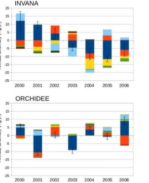
rated wetlands. In this latitudinal band, the signs of the anomalies from 1991 to 2000 for total emissions by the two inversions on the one hand and for wetland emissions by INVANA and ORCHIDEE on the other hand are broadly in agreement. From 2000, and particularly between 2003 and 2006, ORCHIDEE provides anomalies with a sign opposite to the one of INVANA. For example, in 2005 the anomaly at these latitudes is

20

+3 to₊13 Tg y−1_{in ORCHIDEE versus}

−6 to−26 Tg y−1in INVANA (Fig. 1 bottom).

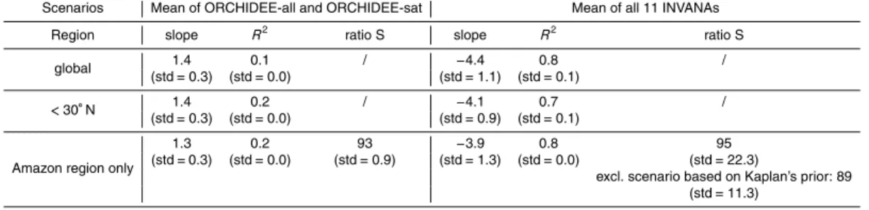
Moreover, the trend over 2000–2006 in this band (Table 1) is₋4.1_±0.9 Tg month−1_for

INVANA whereas the trend for the mean between ORCHIDEE-all (scenario accounting for all wetlands) and ORCHIDEE-sat (scenario with saturated wetlands only) is₊1.4±

0.3 Tg month−1_{(Table 1).}

25

(14)

ACPD

13, 9017–9049, 2013

I. Pison et al.

Title Page

Tables Figures

◭ ◮

Back Close

Full Screen / Esc

Discussion

P

a

per

|

Dis

cussion

P

a

per

|

Discussion

P

a

per

|

Discussio

n

P

a

per

|

of 30◦_{N (Fig. 2). Interestingly, ORCHIDEE and INVANA agree on the fact that}

varia-tions in methane emissions from the Amazon basin (tropical South America in Fig. 2) drive the trend of tropical emissions, but with opposite signs. Indeed, the ratio between the slopes for tropical South America and the whole<30◦_{S region (Table 1) indicates}

that tropical South America explains 93 % of the trend for ORCHIDEE and between

5

89 and 95 % in INVANA (depending on the scenarios). However, the inferred trends for the Amazon region are of opposite signs with −3.9±1.3 Tg y−1 for INVANA and

+1.3_±0.3 Tg y−1_{for ORCHIDEE (Table 1).}

When an atmospheric inversion cannot provide insights about the underlying emis-sion processes and the sensitivity of wetland emisemis-sions to the climate, the ORCHIDEE

10

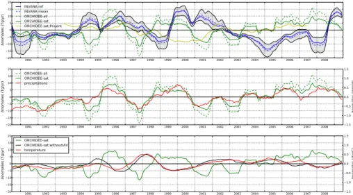
process-based model can. The monthly anomalies of CH₄ wetland emissions for the Amazon region for ORCHIDEE and INVANA, together with the precipitations and tem-perature changes are shown in Fig. 3. Not surprisingly, ORCHIDEE and INVANA phases of the inter-annual variations are not in agreement at this regional scale, al-though the magnitudes of the changes are close. As noted before, the trends between

15

2000 and 2006 are opposite for ORCHIDEE (positive) and INVANA (negative) (Fig. 3, top panel). Wetland extent is a key element in process-model algorithms (Melton et al., 2012). Therefore, in addition to ORCHIDEE-sat where some TOPMODEL concepts are used to compute the variability in time of the wetland extent (Ringeval et al., 2012a), we introduced an ORCHIDEE estimate where this variability is prescribed by the data

20

set by Prigent et al. (2012). Whatever the choice of inter-annual variability (IAV) for wetland extent (i.e. computed or prescribed from remote sensing data), the IAV and the trend in the various ORCHIDEE scenarios are never close to INVANA’s (Fig. 3, upper panel). Interestingly, changing the description of the wetland extent significantly impacts the phasing and the magnitude of the inter-annual variations inferred by

OR-25

(15)

ACPD

13, 9017–9049, 2013

I. Pison et al.

Title Page

Tables Figures

◭ ◮

Back Close

Full Screen / Esc

Discussion

P

a

per

|

Dis

cussion

P

a

per

|

Discussion

P

a

per

|

Discussio

n

P

a

per

|

close to zero for “ORCHIDEE-sat;Prigent” for the period 2002–2005 but remains posi-tive for other ORCHIDEE simulations.

In tropical South America, the trend in ORCHIDEE wetland emissions is driven by precipitations (Fig. 3, middle panel), which show a positive trend of 0.05 mm d−1 be-tween 2000 and 2006 over the Amazon. When the IAV of wetland extent is removed

5

(black curve in Fig. 3, bottom panel), the IAV of emissions over 1990–2009 decreases from 3.8 (ORCHIDEE-sat) to 2.1 Tg y−1 and appears to be driven by air temperature with a strong correlation of 0.86 over 1990–2009 (Fig. 3, bottom panel). Temperature could have an effect on both methanogenesis rate and substrate supply but large un-certainties remain on the contribution of each process (e.g. White et al., 2008, for

10

northern peat-lands).

Overall, ORCHIDEE infers an increase of CH₄ emissions in the Amazon between 2000 and 2006, which is opposite to the decreasing emissions inferred by INVANA inversions. The di_fference of IAV between ORCHIDEE-simulated emissions when the time variability of wetland extent is either prescribed or computed (Fig. 3, upper panel)

15

underlines the difficulty to capture a good IAV of the processes involved in the ex-tension/retraction of wetland areas. A way of improvement would be to implement the floodplains into the model (e.g. like Decharme et al., 2008, 2012), the relevant pro-cesses leading to wetland formation in the Amazon basin (Hess et al., 2003). Un-certainties linked to precipitations (magnitude and spatial distribution) in the Amazon

20

basin and their huge e_ffect on the floodplains extent simulated by land surface models (Guimberteau et al., 2012) is also problematic.

The lack of wetland Plant Functional Type into the ORCHIDEE model and the use of the mean grid-cell simulated labile carbon as methanogenesis substrate’s proxy could also lead to an overestimated sensitivity of CH₄ emissions to precipitations (Ringeval

25

(16)

ACPD

13, 9017–9049, 2013

I. Pison et al.

Title Page

Tables Figures

◭ ◮

Back Close

Full Screen / Esc

Discussion

P

a

per

|

Dis

cussion

P

a

per

|

Discussion

P

a

per

|

Discussio

n

P

a

per

|

The IAV of the remote-sensed inundated extent in the Amazon basin over 2000– 2006 and of the in-situ river discharge are in agreement and do not exhibit a clear negative trend (see Fig. 10a in Papa et al., 2010). This points out at a possible issue with INVANA global inversions. Indeed, the Amazon region is poorly constrained by the surface networks, which only provide routine observations over the neighboring

5

oceans. This lack of nearby observations means that large changes in emissions can be tolerated in the inversion when assimilating these observations. Also, using large regions may induce aggregation errors as explained in Kaminski et al. (2001). It should be noted that for this area INVVAR (which works at the grid cell’s scale but only op-timizes total net emissions) obtains emissions which are close to the prior; the only

10

di_fferences appear in the seasonal time profile, with higher emission peaks, particu-larly in August–September 2005 (a dry year (Frappart et al., 2012) with exceptional fires and September 2007–2008). This seems to confirm that the changes made by INVANA in the large region are due to constraints which are not directly relevant to the Amazon basin.

15

Overcoming the lack of observations requires to assimilate more regional data in the Amazon area (such as aircraft data (Miller et al., 2007), satellite data (for example SCIAMACHY (Frankenberg et al., 2008), IASI (Crevoisier et al., 2009), GOSAT (Morino et al., 2011) (C. Cressot, personal communication, 2012))). It may then be possible to solve the fluxes at the model’s resolution (in INVANA’s set-up) or to solve for the

20

di_fferent source types in the variational approach (with INVVAR method).

In INVANA, if not constrained by nearby measurements, the changes in emissions from the Amazon region are indirectly constrained by the atmospheric growth rate. Global observed concentrations are stable between 2000 and 2006 (Dlugokencky et al., 2009). Bottom-up inventories for anthropogenic emissions give positive trends

25

at the global scale over 2000–2006. For instance, the EDGAR inventory computes a

+8 Tg y−1 _{increase in anthropogenic emissions during this period (EDGAR 4, 2009).}

Consistent with this bottom-up inventory albeit smaller, INVANA infers a+4±2 Tg y−1

(17)

ACPD

13, 9017–9049, 2013

I. Pison et al.

Title Page

Tables Figures

◭ ◮

Back Close

Full Screen / Esc

Discussion

P

a

per

|

Dis

cussion

P

a

per

|

Discussion

P

a

per

|

Discussio

n

P

a

per

|

match the stable global concentration, infers a₋4_±1 Tg y−1_{decrease, mostly in South}

American wetland emissions. This result might be sensitive to the large scale transport between the Northern latitudes and the tropics as stated in Stephens et al. (2007) for carbon dioxide. If the increase in anthropogenic CH₄ emissions is real, a decreasing source or an increasing sink must be identified to match the stable concentrations.

5

There is no indication of a positive trend in OH concentrations after 2000 that could have induced an abnormally increasing methane loss in the troposphere (Rigby et al., 2008; Montzka et al., 2011). The increasing wetland emissions found by ORCHIDEE indicate that South America might only be an opportunistic candidate for reduced emis-sions and that another region and/or another process is indeed decreasing. The

anal-10

yses of 13C in CH₄ recently brought elements to the debate. The possible decrease in microbial-related emissions in the Northern hemisphere since the 1990s inferred by Kai et al. (2011) is contested by the analysis of another more consistent 13C data set, which infers no trend in the inter-hemispheric difference of 13C (Levin et al., 2012). This last result questions the validity of the large increase in anthropogenic methane

emis-15

sions computed by the EDGAR inventory for the early 2000s. Analysis of ethane emis-sions (Aydin et al., 2011; Simpson et al., 2012) or another inventory (IIASA, Lamarque et al., 2010) also point in the direction of non-increasing fossil-fuel-related emissions in the past decades. If anthropogenic emissions are not increasing between 2000 and 2006, one could prescribe stable anthropogenic emissions in INVANA. Then, no

neg-20

atively trending source would be necessary to match the stable CH₄concentrations in INVANA, which could reconcile INVANA and ORCHIDEE.

4 Conclusions

In this study, we bring together two “top-down” and one “bottom-up” approaches. The emissions obtained by the various methods have been compared. They agree on the

25

(18)

stud-ACPD

13, 9017–9049, 2013

I. Pison et al.

Title Page

Tables Figures

◭ ◮

Back Close

Full Screen / Esc

Discussion

P

a

per

|

Dis

cussion

P

a

per

|

Discussion

P

a

per

|

Discussio

n

P

a

per

|

ies, particular events can be identified: the post-Pinatubo years illustrate the impact of tropical wetlands through negative anomalies; the alternate 1997–1998 el-Ni ˜no / 1998– 1999 la-Ni ˜na illustrate the qualitative agreement of all methods with a large impact of wetlands.

A period of poor agreement between T-D and B-U approaches is found between

5

2000 and 2006, during the stagnation of methane atmospheric concentrations. A re-gional analysis indicates that this discrepancy is mostly due to tropical South American wetland emissions. The negative trend in wetland emissions inferred by one set of in-versions is not supported by the ORCHIDEE process-based model, which computes a positive trend in wetland emissions due to increased wetland extent, consistent with

10

the inundated areas retrieved by satellite. This result questions the ability of inver-sions based on surface observations to properly infer emisinver-sions in regions where at-mospheric constraints are sparse, such as South America. It also points to the need to revisit the large increase in anthropogenic emissions computed by some inventories for the early 2000s, which somehow implies to infer a decreasing source to

compen-15

sate and match the stable observed CH₄ concentrations. B-U models have also their owncaveats in tropical regions, such as the non representation of floodplain processes. Regarding the T-D approach, the variational method allows us to assimilate instanta-neous data of any kind. After 2003, satellite data, such as SCIAMACHY, IASI (after 2006) or GOSAT (after 2009), can then be used to constrain methane fluxes in remote

20

areas where surface stations are sparse, particularly at low latitudes (Bergamaschi et al., 2009). Future active missions may also add data at higher latitudes with possibly less biases than former passive retrievals (Heimann and Marshall, 2011).

Acknowledgements. We acknowledge the contributors to the World Data Center for Green-house Gases for providing their data of methane and methyl-chloroform atmospheric

concen-25

trations: AEMET (Agencia Estatal de Meteorologia), AGAGE (Advanced Global Atmospheric Gases Experiment), CSIRO (Commonwealth Scientific and Industrial Research Organisation), Environment Canada, ENEA (Italian National agency for new technologies, Energy and sus-tainable economic development), JMA (Japan Meteorological Agency), LSCE (Laboratoire des Sciences du Climat et de l’Environnement), NIWA (National Institute of Water and

(19)

ACPD

13, 9017–9049, 2013

I. Pison et al.

Title Page

Tables Figures

◭ ◮

Back Close

Full Screen / Esc

Discussion

P

a

per

|

Dis

cussion

P

a

per

|

Discussion

P

a

per

|

Discussio

n

P

a

per

|

spheric Research), NOAA/ESRL (National Oceanic & Atmospheric Administration/Earth Sys-tem Research Laboratory), SAWS (South African Weather Service), UBA (Federal Environment Agency Austria). The authors contacted all data PIs and in particular thank A. J. Gomez-Pelaez (AEMET); R. G. Prinn, R. F. Weiss, H. J. R. Wang (AGAGE); P. Krummel, R. Langenfelds, P. Steele (CSIRO); D. Worthy (EC); S. Piacentino (ENEA); T. Kawasato (JMA); M. Ramonet, M.

5

Schmidt (LSCE); G. Brailsford (NIWA); E. Dlugokencky, S. A. Montzka, G. Dutton (NOAA); E. Brunke (SAWS); K. Uhse (UBA).

We thank N. Viovy (LSCE) for the data for ORCHIDEE forcings and M. Saunois (LSCE) for fruitful discussions. We wish to thank F. Marabelle and his team for computer support at LSCE.

10

The publication of this article is financed by CNRS-INSU.

References

Artuso, F., Chamard, P., Piacentino, S., di Sarra, A., Meloni, D., Monteleone, F., Sferlazzo, D., and Thiery, F.: Atmospheric methane in the Mediterranean: analysis of measurements at the

15

island of Lampedusa during 1995–2005, Atmos. Environ., 41, 3877–3888, 2007. 9024, 9025 Aydin, M., Verhulst, K. R., Saltzman, E. S., Battle, M. O., Montzka, S. A., Blake, D. R., Tang, Q., and Prather, M. J.: Recent decreases in fossil-fuel emissions of ethane and methane derived from firn air, Nature, 476, 198–201, 2011. 9021, 9033

B ˆand ˘a, N., Krol, M., van Weele, M., van Noije, T., and R ¨ockmann, T.: Analysis of global methane

20

changes after the 1991 Pinatubo volcanic eruption, Atmos. Chem. Phys., 13, 2267–2281, doi:10.5194/acp-13-2267-2013, 2013. 9020

Bergamaschi, P., Frankenberg, C., Meirink, J., Krol, M., Villani, M., Houweling, S., Dentener, F.,

(20)

ACPD

13, 9017–9049, 2013

I. Pison et al.

Title Page

Tables Figures

◭ ◮

Back Close

Full Screen / Esc

Discussion

P

a

per

|

Dis

cussion

P

a

per

|

Discussion

P

a

per

|

Discussio

n

P

a

per

|

emissions using SCIAMACHY satellite retrievals, J. Geophys. Res.-Atmos., 114, D22301, doi:10.1029/2009JD012287, 2009. 9034

Bloom, A. A., Palmer, P. I., Fraser, A., Reay, D. S., and Frankenberg, C.: Large-scale controls of methanogenesis inferred from methane and gravity spaceborne data, Science, 327, 322– 325, doi:10.1126/science.1175176, 2010. 9021

5

Bousquet, P., Hauglustaine, D. A., Peylin, P., Carouge, C., and Ciais, P.: Two decades of OH variability as inferred by an inversion of atmospheric transport and chemistry of methyl chlo-roform, Atmos. Chem. Phys., 5, 2635–2656, doi:10.5194/acp-5-2635-2005, 2005. 9023, 9025

Bousquet, P., Ciais, P., Miller, J. B., Dlugokencky, E. J., Hauglustaine, D. A., Prigent, C., Van der

10

Werf, G. R., Peylin, P., Brunke, E. G., Carouge, C., Langenfelds, R. L., Lathiere, J., Papa, F., Ramonet, M., Schmidt, M., Steele, L. P., Tyler, S. C., and White, J.: Contribution of an-thropogenic and natural sources to atmospheric methane variability, Nature, 443, 439–443, doi:10.1038/nature05132, 2006. 9020, 9021

Bousquet, P., Ringeval, B., Pison, I., Dlugokencky, E. J., Brunke, E.-G., Carouge, C.,

Cheval-15

lier, F., Fortems-Cheiney, A., Frankenberg, C., Hauglustaine, D. A., Krummel, P. B., Lan-genfelds, R. L., Ramonet, M., Schmidt, M., Steele, L. P., Szopa, S., Yver, C., Viovy, N., and Ciais, P.: Source attribution of the changes in atmospheric methane for 2006–2008, At-mos. Chem. Phys., 11, 3689-3700, doi:10.5194/acp-11-3689-2011, 2011. 9020, 9021, 9024, 9025, 9032

20

Brunke, E. G., Labuschagne, C., and Scheel, H. E.: Trace gas variations at Cape Point, South Africa, during May 1997 following a regional biomass burning episode, Atmos. Environ., 35, 777–786, 2001. 9024, 9026

Chen, Y.-H. and Prinn, R. G.: Estimation of atmospheric methane emissions between 1996 and 2001 using a three-dimensional global chemical transport model, J. Geophys. Res.,

25

111, D10307, doi:10.1029/2005JD006058, 2006. 9021

Chevallier, F., Fisher, M., Peylin, P., Serrar, S., Bousquet, P., Br ´eon, F.-M., Ch ´edin, A., and

Ciais, P.: Inferring CO2sources and sinks from satellite observations: method and application

to TOVS data, J. Geophys. Res., 110, D24309, doi:10.1029/2005JD006390, 2005. 9023, 9025, 9026

30

(21)

ACPD

13, 9017–9049, 2013

I. Pison et al.

Title Page

Tables Figures

◭ ◮

Back Close

Full Screen / Esc

Discussion

P

a

per

|

Dis

cussion

P

a

per

|

Discussion

P

a

per

|

Discussio

n

P

a

per

|

Cunnold, D., Steele, L., Fraser, P., Simmonds, P., Prinn, R., Weiss, R., Porter, L., O’Doherty, S., Langenfelds, R., Krummel, P., Wang, H., Emmons, L., Tie, X., and Dlugo-kencky, E.: In situ measurements of atmospheric methane at GAGE/AGAGE sites during 1985–2000 and resulting source inferences, J. Geophys. Res.-Atmospheres, 107, 4225, doi:10.1029/2001JD001226, 2002. 9020

5

Decharme, B., Douville, H., Prigent, C., Papa, F., and Aires, F.: A new river flooding scheme for

global climate applications: Off-line evaluation over South America, J. Geophys. Res., 113,

D11110, doi:10.1029/2007JD009376, 2008. 9031

Decharme, B., Alkama, R., Papa, F., Faroux, S., Douville, H., and Prigent, C.: Global

off-line evaluation of the ISBA-TRIP flood model, Clim. Dynam., 38, 1389–1412,

10

doi:10.1007/s00382-011-1054-9, 2012. 9031

Dlugokencky, E., Steele, L., Lang, P., and Masarie, K.: The growth rate and distribution of atmospheric methane, J. Geophys. Res., 99, 1994. 9025, 9026

Dlugokencky, E., Dutton, E. G., Novelli, P. C., Tans, P. P., Masarie, K. A., Lantz, K. O., and

Madronich, S.: Changes in CH4and CO growth rates after the eruption of Mt. Pinatubo and

15

their link with changes in tropical tropospheric UV flux, Geophys. Res. Lett., 23, 2761–2764, doi:10.1029/96GL02638, 1996. 9020

Dlugokencky, E., Masarie, K., Lang, P., and Tans, P.: Continuing decline in the growth rate of the atmospheric methane burden, Nature, 393, 447–450, 1998. 9020

Dlugokencky, E., Myers, R., Lang, P., Masarie, K., Crotwell, A., Thoning, K., Hall, B., Elkins, J.,

20

and Steele, L.: Conversion of NOAA atmospheric dry air CH4mole fractions to a

gravimetri-cally prepared standard scale, J. Geophys. Res, 110, D18306, DOI: 10.1029/2005JD006035, 2005. 9026

Dlugokencky, E., Bruhwiler, L., White, J., Emmons, L., Novelli, P., Montzka, S., Masarie, K., Crotwell, A., Miller, J., and Gatti, L.: Observational constraints on recent increases in the

25

atmospheric CH4 burden, Geophys. Res. Lett., doi:10.1029/2009GL039780, 2009. 9020,

9021, 9025, 9026, 9032

Dlugokencky, E. J., Houweling, S., Bruhwiler, L., Masarie, K. A., Lang, P. M., Miller, J. B., and

Tans, P. P.: Atmospheric methane levels off: temporary pause or a new steady-state?,

Geo-phys. Res. Lett, 30, 1992, doi:10.1029/2003GL018126, 2003. 9020

30

(22)

ACPD

13, 9017–9049, 2013

I. Pison et al.

Title Page

Tables Figures

◭ ◮

Back Close

Full Screen / Esc

Discussion

P

a

per

|

Dis

cussion

P

a

per

|

Discussion

P

a

per

|

Discussio

n

P

a

per

|

D6 pp., available online at: http://adsabs.harvard.edu/abs/2011AGUFM.A51D..06D, 2011. 9020

EDGAR 4: Emission Database for Global Atmospheric Research (EDGAR), release version 4.0., European Commission, Joint Research Centre (JRC)/Netherlands Environmental As-sessment Agency (PBL), available at: http://edgar.jrc.ec.europa.eu (last access: April 2011),

5

2009. 9021, 9022, 9032

EPA: Global Anthropogenic Non-CO2 Greenhouse Gas Emissions: 1990–2030, US

Environ-mental Protection Agency, Washington DC, 20460, report EPA 430-D-11-003. available at: http://www.epa.gov/nonco2/econ-inv/international.html (last access: November 2012), 2011. 9022

10

Folberth, G., Hauglustaine, D., Ciais, P., and Lathi `ere, J.: On the role of atmospheric chemistry

in the global CO2 budget, Geophys. Res. Lett., 32, L08801, doi:10.1029/2004GL021812,

2005. 9026

Francey, R., Steele, L., Langenfelds, R., and Pak, B.: High precision long-term monitoring of radiatively active and related trace gases at surface sites and from aircraft in the Southern

15

Hemisphere atmosphere, J. Atmos. Sci., 56, 279–285, 1999. 9024, 9025

Frankenberg, C., Bergamaschi, P., Butz, A., Houweling, S., Meirink, J., Notholt, J., Pe-tersen, A., Schrijver, H., Warneke, T., and Aben, I.: Tropical methane emissions: a re-vised view from SCIAMACHY onboard ENVISAT, Geophys. Res. Lett, 35, L15811, doi:10.1029/2008GL034300, 2008. 9032

20

Frappart, F., Papa, F., da Silva, J. S., Ramillien, G., Prigent, C., Seyler, F., and Calmant, S.: Surface freshwater storage and dynamics in the Amazon basin during the 2005 exceptional drought, Environ. Res. Lett., 7, 044010, doi:10.1088/1748-9326/7/4/044010, 2012. 9032 Fung, I., John, J., Lerner, J., Matthews, E., Prather, M., Steele, L., and Fraser, P.:

Three-dimensional model synthesis of the global methane cycle, J. Geophys. Res., 96, 13033–

25

13065, 1991. 9026

Gauci, V., Blake, S., Stevenson, D. S., and Highwood, E. J.: Halving of the northern

wet-land CH4 source by a large Icelandic volcanic eruption, J. Geophys. Res., 113, G00A11

doi:10.1029/2007JG000499, 2008. 9020

Gomez-Pelaez, A., Ramos, R., Cuevas, E., and Gomez-Trueba, V.: 25 years of continuous CO2

30

and CH4measurements at Iza ˜na Global GAW mountain station: annual cycles and

(23)

ACPD

13, 9017–9049, 2013

I. Pison et al.

Title Page

Tables Figures

◭ ◮

Back Close

Full Screen / Esc

Discussion

P

a

per

|

Dis

cussion

P

a

per

|

Discussion

P

a

per

|

Discussio

n

P

a

per

|

Mountain Sites (ACP Symposium 2010), Interlaken, Switzerland, 8–10 June 2010, 157–159 pp., 2010. 9024, 9025

Guimberteau, M., Drapeau, G., Ronchail, J., Sultan, B., Polcher, J., Martinez, J.-M., Pri-gent, C., Guyot, J.-L., Cochonneau, G., Espinoza, J. C., Filizola, N., Fraizy, P., Lavado, W., De Oliveira, E., Pombosa, R., Noriega, L., and Vauchel, P.: Discharge simulation in the

sub-5

basins of the Amazon using ORCHIDEE forced by new datasets, Hydrol. Earth Syst. Sci., 16, 911–935, doi:10.5194/hess-16-911-2012, 2012. 9031

Hauglustaine, D., Hourdin, F., Jourdain, L., Filiberti, M., Walters, S., Lamarque, J., and Hol-land, E.: Interactive chemistry in the Laboratoire de M ´et ´eorologie Dynamique general cir-culation model: description and background tropospheric chemistry evaluation, J. Geophys.

10

Res., 109, D04314, doi:10.1029/2003JD003957, 2004. 9026

Heimann, M. and Marshall, J.: CH4 Flux Inversion Studies for Future Active Space CH4

Mis-sions like MERLIN, AGU Fall Meeting Abstracts, C6 pp., available online at: http://adsabs. harvard.edu/abs/2011AGUFM.A34C..06H, 2011. 9034

Hess, L. L., Melack, J. M., Novo, E. M., Barbosa, C. C., and Gastil, M.: Dual-season mapping

15

of wetland inundation and vegetation for the central Amazon basin, Remote Sens. Environ., 87, 404–428, 2003. 9031

Hodson, E. L., Poulter, B., Zimmermann, N. E., Prigent, C., and Kaplan, J. O.: The El Ni ˜no-Southern Oscillation and wetland methane interannual variability, Geophys. Res. Lett., 38, L08810, doi:10.1029/2011GL046861, 2011. 9028

20

Hogan, K. B. and Harriss, R. C.: Comment on “A dramatic decrease in the growth rate of atmospheric methane in the Northern Hemisphere during 1992” by E. J. Dlugokencky et al., Geophys. Res. Lett, 21, 2445–2446, 1994. 9028

Hourdin, F., Musat, I., Bony, S., Braconnot, P., Codron, F., Dufresne, J.-L., Fairhead, L., Filib-erti, M.-A., Friedlingstein, P., Grandpeix, J.-Y., Krinner, G., LeVan, P., Li, Z.-X., and Lott, F.:

25

The LMDZ4 general circulation model: climate performance and sensitivity to parametrized physics with emphasis on tropical convection, Clim. Dynam., 27, 787–813, 2006. 9025 Kai, F. M., Tyler, S. C., Randerson, J. T., and Blake, D. R.: Reduced methane growth rate

explained by decreased Northern Hemisphere microbial sources, Nature, 476, 194–197, 2011. 9021, 9033

30

(24)

ACPD

13, 9017–9049, 2013

I. Pison et al.

Title Page

Tables Figures

◭ ◮

Back Close

Full Screen / Esc

Discussion

P

a

per

|

Dis

cussion

P

a

per

|

Discussion

P

a

per

|

Discussio

n

P

a

per

|

Krinner, G., Viovy, N., de Noblet-Ducoudr ´e, N., Ogee, J., Polcher, J., Friedlingstein, P., Ciais, P., Sitch, S., and Prentice, I.: A dynamic global vegetation model for studies of the coupled atmosphere-biosphere system, Global Biogeochem. Cy., 19, GB1015, doi:10.1029/2003GB002199, 2005. 9023

Lamarque, J.-F., Bond, T. C., Eyring, V., Granier, C., Heil, A., Klimont, Z., Lee, D., Liousse, C.,

5

Mieville, A., Owen, B., Schultz, M. G., Shindell, D., Smith, S. J., Stehfest, E., Van Aar-denne, J., Cooper, O. R., Kainuma, M., Mahowald, N., McConnell, J. R., Naik, V., Riahi, K., and van Vuuren, D. P.: Historical (1850–2000) gridded anthropogenic and biomass burn-ing emissions of reactive gases and aerosols: methodology and application, Atmos. Chem. Phys., 10, 7017-7039, doi:10.5194/acp-10-7017-2010, 2010. 9033

10

Langenfelds, R., Francey, R., Pak, B., Steele, L., Lloyd, J., Trudinger, C., and Allison, C.:

Interannual growth rate variations of atmospheric CO₂ and its δ13C, H₂, CH₄, and CO

between 1992 and 1999 linked to biomass burning, Global Biogeochem. Cy., 16, 1048, doi:10.1029/2001GB001466, 2002. 9020

Lawrence, D. M. and Slater, A. G.: Incorporating orgainc soil into a global climate model, Clim.

15

Dynam., 30, 145–160, doi:10.1007/s00382-007-0278-1, 2007. 9024

Levin, I., Veidt, C., Vaughn, B. H., Brailsford, G., Bromley, T., Lowe, R. H. D., Miller, J. B.,

Poß, C., and White, J. W. C.: No inter-hemispheric δ13_CH₄ _{trend observed, Nature, 486,}

E3–E4, doi:10.1038/nature11175, 2012. 9021, 9033

Lowe, D., Brenninkmeijer, C., Tyler, S., and Dlugkencky, E.: Determination of the isotopic

com-20

position of atmospheric methane and its application in the Antarctic, J. Geophys. Res., 96, 15455–15467, 1991. 9024, 9026

Matsueda, H., Sawa, Y., Wada, A., Inoue, H. Y., Suda, K., Hirano, Y., Tsuboi, K., and Nish-ioka, S.: Methane standard gases for atmospheric measurements at the MRI and JMA and intercomparison experiments, Pap. Meteorol. Geophys., 54, 91–109, 2004. 9024, 9026

25

Matthews, E. and Fung, I.: Methane emission from natural wetlands: Global distribution, area, and environmental characteristics of sources, Global Biogeochem. Cy., 1, 61–86, doi:10.1029/GB001i001p00061, 1987. 9025

Melton, J. R., Wania, R., Hodson, E. L., Poulter, B., Ringeval, B., Spahni, R., Bohn, T., Avis, C. A., Beerling, D. J., Chen, G., Eliseev, A. V., Denisov, S. N., Hopcroft, P. O.,

Let-30

(25)

ACPD

13, 9017–9049, 2013

I. Pison et al.

Title Page

Tables Figures

◭ ◮

Back Close

Full Screen / Esc

Discussion

P

a

per

|

Dis

cussion

P

a

per

|

Discussion

P

a

per

|

Discussio

n

P

a

per

|

(WETCHIMP), Biogeosciences, 10, 753–788, doi:10.5194/bg-10-753-2013, 2013. 9022, 9030

Miller, J., Gatti, L., d’Amelio, M., Crotwell, A., Dlugokencky, E., Bakwin, P., Artaxo, P., and Tans, P.: Airborne measurements indicate large methane emissions from the eastern Ama-zon basin, Geophys. Res. Lett, 34, doi:10.1029/2006GL029213, 2007. 9032

5

Monteil, G., Houweling, S., Dlugockenky, E. J., Maenhout, G., Vaughn, B. H., White, J. W. C., and Rockmann, T.: Interpreting methane variations in the past two decades using

measure-ments of CH4mixing ratio and isotopic composition, Atmos. Chem. Phys., 11, 9141–9153,

doi:10.5194/acp-11-9141-2011, 2011. 9021

Montzka, S., Spivakovsky, C., Butler, J., Elkins, J., Lock, L., and Mondeel, D.: New observational

10

constraints for atmospheric hydroxyl on global and hemispheric scales, Science, 288, 500– 503, doi:10.1126/science.288.5465.500, 2000. 9025, 9026

Montzka, S., Krol, M., Dlugokencky, E., Hall, B., J ¨ockel, P., and Lelieveld, J.: Small interannual variability of global atmospheric hydroxyl, Science, 331, 67–69, doi:10.1126/science.1197640, 2011. 9021, 9025, 9026, 9028, 9033

15

Morino, I., Uchino, O., Inoue, M., Yoshida, Y., Yokota, T., Wennberg, P. O., Toon, G. C.,

Wunch, D., Roehl, C. M., Notholt, J., Warneke, T., Messerschmidt, J., Griffith, D. W. T.,

Deutscher, N. M., Sherlock, V., Connor, B., Robinson, J., Sussmann, R., and Rettinger, M.: Preliminary validation of column-averaged volume mixing ratios of carbon dioxide and methane retrieved from GOSAT short-wavelength infrared spectra, Atmos. Meas. Tech., 4,

20

1061–1076, doi:10.5194/amt-4-1061-2011, 2011. 9032

NOAA: NOAA data website, available at: http://www.esrl.noaa.gov/gmd/dv/ftpdata.html, last ac-cess: 2 April 2012. 9024

Olivier, J. G. J. and Berdowski, J. J. M.: The Climate System, chap. Global emissions sources and sinks, edited by: Berdowski, J., Guichert, R., Heij, B., A. A. Balkema/Swets & Zeitlinger,

25

33–37 pp., 2001. 9025, 9026

Papa, F., Prigent, C., Aires, F., Jimenz, C., Rossow, W., and Matthews, E.: Interannual variability of surface water extent at the global scale, 1993–2004, J. Geophys. Res., 115, D12111, doi:10.1029/2009JD012674, 2010. 9023, 9032, 9049

Peylin, P., Bousquet, P., Ciais, P., and Monfray, P.: Inverse methods in global biogeochemical

30

(26)

ACPD

13, 9017–9049, 2013

I. Pison et al.

Title Page

Tables Figures

◭ ◮

Back Close

Full Screen / Esc

Discussion

P

a

per

|

Dis

cussion

P

a

per

|

Discussion

P

a

per

|

Discussio

n

P

a

per

|

Peylin, P., Baker, D., Sarmiento, J., Ciais, P., and Bousquet, P.: Influence of transport

uncer-tainty on annual mean and seasonal inversions of atmospheric CO2data, J. Geophys.

Res.-Atmos., 107, 4385, doi:10.1029/2001JD000857, 2002. 9025

Pison, I., Bousquet, P., Chevallier, F., Szopa, S., and Hauglustaine, D.: Multi-species inversion

of CH4, CO and H2emissions from surface measurements, Atmos. Chem. Phys., 9, 5281–

5

5297, doi:10.5194/acp-9-5281-2009, 2009. 9023, 9025, 9026

Prigent, C., Papa, F., Aires, F., Jimenez, C., Rossow, W. B., and Matthews, E.: Changes in land surface water dynamics since the 1990s and relation to population pressure, Geophys. Res. Lett., 39, L08403, doi:10.1029/2012GL051276, 2012. 9023, 9030

Prinn, R., Weiss, R., Fraser, P., Simmonds, P. G., Cunnold, D., Alyea, F., O’Doherty, S.,

10

Salameh, P., Miller, B., Huang, J., Wang, R., Hartley, D., Harth, C., Steele, L., Sturrock, G., Midgley, P. M., and McCulloch, A.: A history of chemically and radiatively important gases in air deduced from ALE/GAGE/AGAGE, J. Geophys. Res., 115, 17751–17792, 2000. 9024 Prinn, R., Huang, J., Weiss, R., Cunnold, D. M., Fraser, P., Simmonds, P., McCulloch, A.,

Harth, C., Reimann, S., Salameh, P., O’Doherty, S., Wang, R., Porter, L., Miller, B., and

15

Krummel, P.: Evidence for variability of atmospheric hydroxyl radicals over the past quarter century, Geophys. Res. Lett., 32, L07809, doi:10.1029/2004GL022228, 2005. 9025

Prinn, R. G., Weiss, R. F., Fraser, P. J., Simmonds, P. G., Cunnold, D. M., O’Doherty, S., Salameh, P. K., Porter, L. W., Krummel, P. B., Wang, R. H. J., Miller, B. R., Harth, C., Gre-ally, B. R., Woy, F. A. V., Steele, L. P., M ¨uhle, J., Sturrock, G. A., Alyea, F. N., Huang, J.,

20

and Hartley, D. E.: AGAGE data base, Tech. rep., The ALE/GAGE/AGAGE Network, http: //agage.eas.gatech.edu/index.htm, last access: 31 March 2012. 9024

Rigby, M., Prinn, R., Fraser, P., Simmonds, P., Langenfelds, R., Huang, J., Cunnold, D., Steele, L., Krummel, P., Weiss, R., O’Doherty, S., Salameh, P., Wang, H., Harth, C., M ¨ulhe, J., and Porter, L.: Renewed growth of atmospheric methane, Geophys. Res. Lett., 35, L22805,

25

doi:10.1029/2008GL036037, 2008. 9020, 9021, 9025, 9033

Ringeval, B., de Noblet-Ducoudr ´e, N., Ciais, P., Bousquet, P., Prigent, C., Papa, F., and Rossow, W.: An attempt to quantify the impact of changes in wetland extent on methane emissions at the seasonal and interannual time scales, Global Biogeochem. Cy., 24, GB2003, doi:10.1029/2008GB003354, 2010. 9021, 9023

30

Ringeval, B., Friedlingstein, P., Koven, C., Ciais, P., de Noblet-Ducoudr ´e, N., Decharme, B., and

Cadule, P.: Climate-CH4 feedback from wetlands and its interaction with the climate-CO2

(27)

ACPD

13, 9017–9049, 2013

I. Pison et al.

Title Page

Tables Figures

◭ ◮

Back Close

Full Screen / Esc

Discussion

P

a

per

|

Dis

cussion

P

a

per

|

Discussion

P

a

per

|

Discussio

n

P

a

per

|

Ringeval, B., Decharme, B., Piao, S. L., Ciais, P., Papa, F., de Noblet-Ducoudr ´e, N., Prigent, C., Friedlingstein, P., Gouttevin, I., Koven, C., and Ducharne, A.: Modelling sub-grid wetland in the ORCHIDEE global land surface model: evaluation against river discharges and remotely sensed data, Geosci. Model Dev., 5, 941–962, doi:10.5194/gmd-5-941-2012, 2012a. 9023, 9030

5

Ringeval, B., Hopcroft, P. O., Valdes, P. J., Ciais, P., Ramstein, G., Dolman, A. J., and Kageyama, M.: Response of methane emissions from wetlands to the Last Glacial Maximum

and an idealized Dansgaard–Oeschger climate event: insights from two models of different

complexity, Clim. Past, 9, 149–171, doi:10.5194/cp-9-149-2013, 2013. 9031

Schmidt, M., Ramonet, M., Wastine, B., Delmotte, M., Galdemard, P., Kazan, V., Messager, C.,

10

Royer, A., Valant, C., Xueref, I., and Ciais, P.: RAMCES: The French Network of Atmospheric Greenhouse Gas Monitoring, in: 13th WMO/IAEA Meeting of Experts on Carbon Dioxide Concentration and Related Tracers Measurement Techniques, GAW report No. 168 (2006), Boulder, Colorado, USA, 165–174 pp., 2005. 9024, 9025, 9026

Simpson, I. J., Andersen, M. P. S., Meinardi, S., Bruhwiler, L., Blake, N. J., Helmig, D.,

Row-15

land, F. S., and Blake, D. R.: Long-term decline of global atmospheric ethane concentrations and implications for methane, Nature, 488, 490–494, doi:10.1038/nature11342, 2012. 9021, 9033

Stephens, B. B., Gurney, K. R., Tans, P. P., Sweeney, C., Peters, W., Bruhwiler, L., Ciais, P., Ramonet, M., Bousquet, P., Nakazawa, T., Aoki, S., Machida, T., Inoue, G.,

20

Vinnichenko, N., Lloyd, J., Jordan, A., Heimann, M., Shibistova, O., Langenfelds, R. L., Steele, L. P., Francey, R. J., and Denning, A. S.: Weak northern and strong tropical

land carbon uptake from vertical profiles of atmospheric CO2, Science, 316, 1732–1735,

doi:10.1126/science.1137004, 2007. 9033

Sussmann, R., Forster, F., Rettinger, M., and Bousquet, P.: Renewed methane increase for five

25

years (2007—2011) observed by solar FTIR spectrometry, Atmos. Chem. Phys., 12, 4885– 4891, doi:10.5194/acp-12-4885-2012, 2012. 9021

UBA: UBA website, available at: http://www.umweltbundesamt.de/luft/luftmessnetze/

ubamessnetz.htm (last access: 2 April 2013), 2013. 9024, 9026

Uppala, S. M., K ˚Allberg, P. W., Simmons, A. J., Andrae, U., Bechtold, V. D. C., Fiorino, M.,

Gib-30