Large-scale and synoptic meteorology in the south-east Pacific during the observations campaign VOCALS-REx in austral Spring 2008

www.atmos-chem-phys.net/11/4977/2011/ doi:10.5194/acp-11-4977-2011

© Author(s) 2011. CC Attribution 3.0 License.

Chemistry

and Physics

Large-scale and synoptic meteorology in the south-east Pacific

during the observations campaign VOCALS-REx in austral

Spring 2008

T. Toniazzo1, S. J. Abel2, R. Wood3, C. R. Mechoso4, G. Allen5, and L. C. Shaffrey1 1_{NCAS, Department of Meteorology, University of Reading, RG6 6BB, UK}

2_{Met Office, Exeter, UK}

3_{University of Washington, Seattle, USA} 4_{UCLA, Los Angeles, USA}

5_{University of Manchester, UK}

Received: 30 November 2010 – Published in Atmos. Chem. Phys. Discuss.: 6 January 2011 Revised: 26 April 2011 – Accepted: 5 May 2011 – Published: 27 May 2011

Abstract. We present a descriptive overview of the me-teorology in the south eastern subtropical Pacific (SEP) during the VOCALS-REx intensive observations campaign which was carried out between October and November 2008. Mainly based on data from operational analyses, forecasts, reanalysis, and satellite observations, we focus on spatio-temporal scales from synoptic to planetary. A climatologi-cal context is given within which the specific conditions ob-served during the campaign are placed, with particular ref-erence to the relationships between the large-scale and the regional circulations. The mean circulations associated with the diurnal breeze systems are also discussed. We then pro-vide a summary of the day-to-day synoptic-scale circulation, air-parcel trajectories, and cloud cover in the SEP during VOCALS-REx. Three meteorologically distinct periods of time are identified and the large-scale causes for their dif-ferent character are discussed. The first period was char-acterised by significant variability associated with synoptic-scale systems interesting the SEP; while the two subsequent phases were affected by planetary-scale disturbances with a slower evolution. The changes between initial and later pe-riods can be partly explained from the regular march of the annual cycle, but contributions from subseasonal variability and its teleconnections were important. Across the whole of the two months under consideration we find a significant correlation between the depth of the inversion-capped ma-rine boundary layer (MBL) and the amount of low cloud in the area of study. We discuss this correlation and argue that

Correspondence to:T. Toniazzo ([email protected])

at least as a crude approximation a typical scaling may be ap-plied relating MBL and cloud properties with the large-scale parameters of SSTs and tropospheric temperatures. These results are consistent with previously found empirical rela-tionships involving lower-tropospheric stability.

1 Introduction

The marine stratocumulus (Sc) systems of the subtropical anticyclones cause a large negative radiative forcing for the global climate system (Klein and Hartmann, 1993). They are also associated with oceanic upwelling systems of enormous biological productivity (e.g. Hastenrath, 1991: Sect. 10.5, and references therein). Such associations make them fun-damentally important building blocks of the present-day cli-mate system.

are sensitive to local feedbacks between radiation and tur-bulence in the maritime boundary-layer (MBL) that tend to exacerbate errors (Konor et al., 2009).

In part to address some of these issues, a concentrated observational and modelling study has been underway that focuses on the south-eastern Pacific (SEP) off the western coast of South America, where the most persistent tropi-cal Sc decks are found (Klein and Hartmann, 1993). The international research project, called VOCALS (VAMOS ocean-cloud-atmosphere-land study), included an intensive observations campaign in the SEP (VOCALS-REx), between 1 October and 2 December 2008. An introduction to VO-CALS, and a detailed overview of VOCALS-REx operations and observations, is provided in Wood et al. (2011).

Our primary goal in this contribution is to provide a mete-orological context for VOCALS-REx observations. In doing so we aim to highlight the role of synoptic and large-scale atmospheric forcing in controlling changes to the Sc deck. This question is complementary to and thus addresses one of the core science questions of VOCALS, namely to what extent cloud microphysical processes, including aerosol in-teraction, affect the cloud cover in tropical Sc areas. Several studies have already highlighted the importance of dynami-cally forced cloud variability.

Garreaud et al. (2002) have shown that sub-synoptic sys-tems that arise from the interaction between synoptic forcing and the Andean orography significantly affect Sc cover over time-scales of a few days. From their analysis of satellite and sea-level pressure data, George and Wood (2010) have argued that, more generally, sub-seasonal variability in cloud properties is to a significant extent controlled by meteoro-logical conditions. In the context of VOCALS-REx, Rahn and Garreaud (2010b) have shown that the observed variabil-ity in MBL depth, and in part of the associated cloud cover, was largely dependent on synoptic forcing in the SEP area. Additional evidence of meteorological controls is given in Zuidema et al. (2009) and Painemal et al. (2010).

By using a variety of observational, reanalysis, and opera-tional analysis/forecast data, in this contribution we synthe-sise the available meteorological information for the dura-tion of the VOCALS-REx campaign. We provide an exhaus-tive documentation of the meteorology from sub-synoptic to planetary scales which may constitute a background for fu-ture VOCALS modelling case-studies. We then exploit this descriptive analysis to discuss the relationship between the synoptic- and large-scale circulation and the observed state and variability of the MBL and cloud in the VOCALS-REx domain, with the aim to attempt to isolate and quantify, from a large-scale perspective, the dynamically induced part of the observed cloud variability. Reflecting these different aims, the paper is structured in several inter-dependent sections, in an order meant to provide a context for each part of the mete-orological analysis we conducted. We summarise them here to provide a guide to the reader.

Section 2 details the data we used for this analysis. In Sect. 3 we provide the background context for VOCALS-REx with a description of the mean circulation and the as-sociated typical meteorological conditions for the area of the southern Pacific subtropical anticyclone observed by VOCALS-REx. Section 4 complements this with a descrip-tion of the mean diurnal variadescrip-tions of the circuladescrip-tion in the SEP, which are of obvious importance for the specific tem-poral sampling of VOCALS-REx missions. These two initial sections complement the discussion on the general meteorol-ogy of the SEP given in other literature (Rahn and Garreaud, 2010a; Zuidema et al., 2009) and is also required in order to provide the context for the subsequent sections in this paper. We then move to the planetary scales circulation in Sect. 5, where we describe its seasonal evolution and its likely drivers for October–November 2008. In Sect. 6 we discuss regional and remote large-scale inter-annual and sub-seasonal anoma-lies that affected the VOCALS-REx campaign. Section 7 fi-nally focuses on the region of the south-east Pacific sampled during VOCALS-REx, with specific attention to the cloud cover and to the circulation and tracer advection in the lower troposphere and the MBL. This is the part most closely rel-evant for VOCALS-REx operations and is descriptive in na-ture, with a nearly day-to-day assessment of the meteorol-ogy. We discuss the evolution of the MBL during VOCALS-REx and the connection between local and large scales in Sect. 8. This part addresses the broader scientific aims of VOCALS, by investigating how the state of the MBL and of the cloud cover in the SEP are related in a general sense with the synoptic- and planetary-scale conditions. Finally, Sect. 9 summarises our findings and draws conclusions.

2 Data sources

We base most of the following discussion on data from the analysis fields and 21-h forecasts (at 3-hourly intervals) of the UK Met Office global operational forecast model (cy-cle G48, operational from July to November 2008). It uses a 4D-Var variational data assimilation system (Rawlins et al., 2007) which includes perturbation forecasts and adjoint models to obtain the optimal representation of the meteoro-logical conditions within a 6-h data window.

sea-level) above level 30 (17.4 km). The dynamical core is based on a non-hydrostatic, two-time level, semi-implicit, semi-Lagrangian high-order (cubic to quintic) formulation (Davies et al., 2005). The boundary layer scheme is a nonlocal surface-forced K-profile scheme based on Lock et al. (2000); the microphysics scheme is based on Wil-son and Ballard (1999); and the cloud fraction scheme on Smith (1990). The two-stream radiation scheme, based on Edwards and Slingo (1996), is called every three hours. The model physical parameterisations are similar to those used in the Met Office Hadley Centre atmospheric climate model HadGEM1 (Martin et al., 2006).

A validation of the UKMO global forecast system for the SEP area is given Wyant et al. (2010; the preVOCA study). They find that this system has skill in MBL and cloud fore-casts over a time-span well in excess of the 21-h horizon we consider here. The only other operational model to show a good performance among the 6 tested was the ECMWF system. Problems were identified with the representation of MBL adjacent to the South-American coast, where is it too shallow and lacking cloud.

Here we consider data for the whole of October and November 2008. Whenever possible, we base our findings on the data from the operational analyses at 00:00 UTC.

We have also analysed the analysis and forecast fields gen-erated with the limited-area configuration of the UKMO fore-cast system that was integrated over 37 days (between 14 Oc-tober and 19 November) over the SEP region (Abel et al., 2010). Abel et al. (2010) provide a validation of the model for this period, and show that, in general, the forecast fields are consistent with in-situ observations when maritime eas well away from the coast are considered. Over such ar-eas, the differences between the limited-area model and the lower-resolution global operational forecast model are quite minor for all the purposes of our discussion. For example, the differences in low-cloud cover, which is one of the more sensitive fields, can be appreciated from Figs. 18 and 22 in Sect. 8. There is generally higher cloud-cover in the limited-area model, correcting some of the bias in the global model, but the spatial and temporal variations are extremely similar. Consistently with these results, we mostly focus the present study on the maritime areas of the SEP. We also give a preference for the analysis of the global forecast and reanal-ysis data over the limited-are products, because they have the desired temporal coverage including all of the VOCALS-REx period, and provide a degree of internal consistency across the circulations at all the spatial scales under discus-sion here.

In addition to UKMO operational data, we use the ERA-Interim reanalysis (Simmons et al., 2006) product and op-erational analyses (cycle 36r4, used here for the back-trajectories) of the ECMWF (European Centre for Medium-Range Weather Forecast). The former is used for the discus-sion of the global climatology for austral Spring. No signif-icant differences between the UKMO operational analyses

and ERA-Interim were seen over the October and Novem-ber 2008 that would impact our discussion, and for consis-tency we generally show UKMO data for that period.

Finally, we will refer to datasets obtained from the obser-vational activities of the VOCALS-REx campaign. These include cloud-cover estimates from visible and infred ra-diance observations by the NOAA geostationary meteoro-logical satellite GOES-10. In addition, we use ship-based radiosonde profiles, and measurements of SSTs, surface air temperatures and winds (see Wood et al., 2011; cf. also Zuidema et al., 2009; Bretherton et al., 2010), and the satellite-derived SST products OSTIA from the UK Met Of-fice (Stark et al., 2007) and the Optimal Interpolation from NOAA (Reynolds et al., 2002).

3 The average atmospheric circulation in the SEP

The VOCALS-REx campaign, which took place in the pe-riod between 1 October and 2 December 2008, sampled the eastern flank of the subtropical high pressure system of the southeastern Pacific (SEP).

At the deepest point of the wide bay formed by the south-ern Peruvian and northsouth-ern Chilean coast-lines, the town of Arica (18◦S, 70◦W) served as the main operational base of VOCALS-REx. Observations were gathered mostly in the vicinity of 20◦S, between 72◦W, near the Chilean coast, and a western-most point at 85◦W where an oceanographic buoy operated by the Woods Hole Oceanographic Institution is lo-cated. Along and within a range of 200–300 km of the coast, ground-, aircraft- and ship-based activities sampled atmo-spheric data between 30◦S and 13◦S. This strip of intensive observations is marked in the panels of Fig. 1 by the thick, dashed white line. Wood et al. (2011) gives a comprehensive description of VOCALS-REx operations.

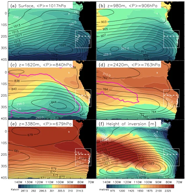
Fig. 1. (a)to (e)Potential temperature (colour-coded, dotted contours, in K) and pressure (full black lines, in hPa) for the October– November 2008 mean in the south-east Pacific, at the surface and four different altitudes, as indicated. The pink contour lines in the third and fourth panels indicates where the diagnosed inversion intersects the horizontal section. The white box with the thick dashed line along 20◦S marks the area where VOCALS-REx operations took place. The colour scale is shown in the bar at the bottom of panel(e).(f)Mean height of the diagnosed inversion (colours, in m; colour scale at the bottom of this panel), when present (positive vertical temperature gradient); the black contours show the surface pressure, and are identical to those in panel(a). All data from the UKMO global operational analysis (00:00 UTC).

the short-wave (SW) radiation absorbed by the ocean by an amount of the order of one hundred W m−2(e.g. Colbo and Weller, 2007). The positive residual net heat flux into the ocean (Colbo and Weller, 2007; de Szoeke et al., 2010) is offset by cold oceanic advection, aided by the wind-forced coastal upwelling. The relative role of each of these pro-cesses to maintain the observed thermal and dynamical state of the MBL in the SEP has long been the subject of active investigation (e.g. Ma et al., 1996; Zheng et al., 2010).

Fig. 2. (a)Total (thick black lines) and zonally asymmetric com-ponent (colours) of the 500–700 hPa geopotential thickness fields in the eastern-Pacific/south-American sector. (b)Same as(a), but for the 200–500 hPa thickness. Shown are the time-means for the period between 1 October 2008 and 30 November 2008. For the total thickness, the contour interval is 20 m in panel(a), and 40 m in panel(b). Data from UKMO operational analysis.

differences, and the inversion height at any given point in time and space corresponds to one of the model half-levels. The inversion is diagnosed to exist at a given location and time if the vertical gradient of air temperature is positive.

The level of the MBL-top inversion represents the scale-height of the cold surface anticyclone, which disappears above 700 hPa (Fig. 1e). East of the surface anticyclone, the mean wind veers from a southerly flow in the MBL to westerly flow above 700 hPa. At the northern edge of the anticyclone, near 20◦S where VOCALS-REx took place, the mean MBL winds also have a significant easterly component, while above the inversion in the FT there is a weak mean northerly component. Directional variability is extremely

small in the MBL, but it is generally much more pronounced on synoptic time-scales in the FT. To leading order, the ther-mal wind in the lower troposphere in the SEP reflects thick-ness variations of the cool MBL (Fig. 1c, d, and f), rather than horizontal gradients in the MBL temperature itself.

The surface flow is dynamically coupled with the subtrop-ical jet stream in the upper troposphere (Fig. 2b). Condi-tions in the SEP are influenced by the transport of momen-tum and tracers in and across the jet stream, and their vari-ability is directly affected by baroclinic activity in the south-ern mid-latitudes. Of particular interest are the occurrences of coastally-intensified cyclones, or coastal lows, which ini-tially develop upstream of the SEP and are affected by the Andean orography. In association with such disturbances, trailing cold fronts are observed as far north as 20◦S between autumn and spring (Seleuchi et al., 2006; Barret et al., 2009; Rahn and Garreaud, 2010b; a specific case occurred during VOCALS-REx in 23–24 October).

At tropical latitudes, prominent regional features of the circulation in the free troposphere are associated with the heat sources over the elevated topography of the Andes, es-pecially the Peruvian Andes and the Bolivian altiplano, and over areas of moist convection in the Atlantic Warm Pool and the Amazon basin. A Gill-Matsuno (Matsuno, 1966; Gill, 1980) double-anticyclone pattern is visible in Fig. 2b. Its southern branch appears reinforced by the shallower heating over the Andes (Fig. 2a) and results in an anticyclonic turn-ing of the upper-tropospheric winds above the SEP near the continent. As the spring season progresses, insolation and convective activity gradually increase and move southwards, resulting in a strengthening and a southward extension of the pattern shown in Fig. 2b. As well as on the mean circulation, in Sect. 4 we speculate that this also affects the character of the diurnal cycle over the SEP.

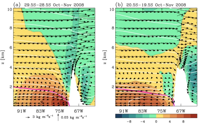
Fig. 3. Meridional transects of mean winds and isoentropes during October–November 2008. Winds are multiplied by density to give mass fluxes. Colour-coding shows zonal wind-speed, with contour interval of 2 kg m−2s−2; white lines are contours for the dry potential temperature, with a spacing of 5 K. Vector scales for the meridional and the vertical winds are given on the bottom-right.(a)Section along 80◦W.(b)Section along 73◦W. The purple line marks the location of the inversion. Means from 3-hourly UKMO operational analysis and 3 h–21 h forecasts are used.

westerly circulation, which increasingly prevails aloft and offshore, the air-masses lofted in the convective activity over the Peruvian Andes and the Amazon can be carried as far as the VOCALS-REx area around 20◦S (see later discussion in Sect. 7.2). South of 30◦S mid-tropospheric ascent becomes noticeable (Fig. 3b), and is associated with the large-scale orographic wave, with a possible contribution from mid-latitude baroclinic activity.

Figure 4 shows zonal transects of the mean circulation in the SEP. Considering first the section along 29◦S, the flow is characterised by mean westerlies aloft and easterlies in the MBL. The mean vertical wind is downward everywhere ex-cept near the orography, with a distinct poleward barrier flow that allows for vortex stretching. Due to the high stability in the free troposphere, the flow across the Andes is subcriti-cal in terms of its Froude number. It Rossby number how-ever is on average close to one, with a characteristic pres-sure maximum above and upstream of the ridge in balance with the southerly wind component which extends the bar-rier flow along the western flanks aloft and eastwards. The increases pressure upstream of the orography associated with the zonal flow affects the pressure distribution at the surface (Richter and Mechoso, 2006) and contributes to the surface divergence in the VOCALS-REx area.

Associated with the south-American land-mass there is a mean temperature front across the mountain chain, and the positive zonal temperature gradient is consistent with the northerly thermal wind component. Along the eastern flanks of the orographic ridge there is a mean updraught that bal-ances the mean diabatic heating, and is associated with a low-level southerly flow. On the western slopes, consistently with the prevailing dry conditions, the warmer air temperatures in proximity of the terrain are associated with mean descent, as shown in Fig. 4. The time-average however hides the vigor-ous diurnal land-sea and mountain breeze circulations, which are associated with descent in the early part of the day and ascent later (see Sect. 4). The presence of a distinct coastal orographic range and of a narrow coastal plateau should be noted here, which are not well-represented in the forecast fields. As a result the near-surface winds near the coast are not accurate (Abel et al., 2010). Such errors may also af-fect the MBL adjacent to land, which is typically too shallow compared to observations (Wyant et al., 2010; Bretherton et al., 2010).

Fig. 4.As in Fig. 3, but for zonal transects along(a)29◦S, and along(b)20◦S (right). Vectors for the vertical and zonal component (scales below panela), colour-coding for the meridional component. Contour intervals are the same as in Fig. 3.

land-mass, and is consistent with Sverdrup vorticity balance below the level of maximum radiatively driven subsidence (around 500 hPa).

Along 20◦S, where most VOCALS-REx observations were taken, the mean flow is similar, but with some differ-ences. Near the northern edge of the anticyclone and of the subtropical jet, the MBL wind has turned, with a stronger but also more divergent zonal flow. The meridional component of the flow is less pronounced, with the maximum wind well away from the coast and no persistent coastal jet. Above the MBL and below the level of the orographic ridge the winds are weaker than at 30◦S.

The flow across the orography has smaller Rossby num-bers (partly also due to the wider orographic ridge), and is as-sociated with a weak mean southerly component, suggesting planetary potential vorticity balance. Below the level of the ridge, the flow appears blocked, and west of the coast there still is a northerly barrier flow. Close to land the mean flow appears to turn southerly, in association with a strong mean upslope wind, suggesting a mean, buoyant surface density current, which converges over the high plateau of the Boli-vian Altiplano. Above the upslope surface current, however, there is strong mean descent, possibly maintaining mass con-tinuity with the zonal flow deceleration aloft. The diabatic forcing associated with the diurnal cycle is likely to be im-portant for the observed mean thermal structure and mean

flow. In addition, variability on synoptic time-scales is asso-ciated not only with variations in the zonal wind speed, but also with changes, sometimes even in sign, of the meridional and vertical wind components, as the dynamical character of the flow across the orography changes. In general, strength-ened zonal flow is associated with enhanced orographic drag and increasing upward and poleward motion over the coastal ocean.

Aloft, the isoentropes have a nearly constant slope and the winds turn northerly everywhere. With a warmer free tropo-sphere and similar MBL temperatures, the inversion is much stronger at 20◦S than at 30◦S, and the cloud cover more per-sistent. Additional features of the flow near 20◦S arise due to the proximity of the Peruvian orography, which is oriented at an angle along the WNW-ESE direction and intercepts the mean southerly flow in the MBL and the lower FT. The circu-lation near this ridge has a vigorous diurnal cycle, with larger diurnal variations than those associated with the N-S Andean crest.

4 Diurnal cycle

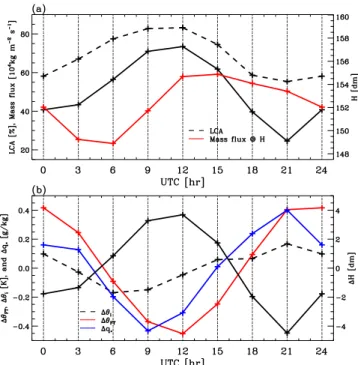
Fig. 5. Mean diurnal evolution of thermodynamic quantities near the inversion in the area 15◦S–25◦S, 90◦W–80◦W.(a)Inversion height (solid black line), cloud amount (broken line), and diagnosed mass entrainment across the inversion (red line) as a function of time of the day. (b) Inversion height anomalies (solid line) to-gether with the lower-tropospheric (z=2200 m) potential temper-ature (red line), the MBL-top potential tempertemper-ature (broken line), and the MBL-top saturation mixing ratio (blue line) as a function of the time of the day. Data from the UKMO operational analyses and 3 h–21 h forecasts.

MBL, owing to the absence of local moist convection. With increased day-time insolation the cloud-top warms and the inversion sinks, with a concomitant reduction in LWP and reduced cloud cover. This process is very important in terms of insolation at the sea surface, as the diurnal cloud-cover minimum occurs a few hours after the maximum in solar ir-radiation.

The UKMO forecast model relies on MBL turbulence parametrisations to represent the processes that drive the di-urnal cycle in the MBL. The simulated a didi-urnal cycle in fractional cloud-cover and MBL depth is in good qualitative agreement with observations, as long as only marine areas well away from the coast are considered (Abel et al., 2010). The simulated mean diurnal variations have the same qualita-tive character as an adiabatic night-time lifting and day-time sinking of the cloud top, concomitant with a reduction or in-crease, respectively, of the lower-tropospheric temperature, and an increase and reduction, respectively, of the cloud liq-uid water concentration (Fig. 5). This may be contrasted with the variability on synoptic time-scales, which lead (Sect. 8) to a correlation between changes in cloud cover and in the inversion height of the opposite sign.

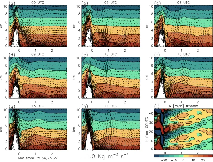
Superimposed on this locally, radiatively driven diurnal cycle, a number of authors (Garreaud and Munoz, 2004; Wood et al., 2009; Rahn and Garreaud, 2010a) have studied the diurnal modulation of the vertical wind in the SEP by regular gravity-wave pulses propagating offshore from the South-American coast. Such pulses affect the entire depth of the troposphere. They are associated with diurnal heat-ing over the Andean mountain ranges, and they have a mea-surable effect on lower-tropospheric temperatures and the MBL-depth (Garreaud and Munoz, 2004), and on cloud liq-uid water (Wood et al., 2002; O’Dell et al., 2008). Figure 6 shows the associated, daily circulation anomalies for a tran-sect along a great circle that intertran-sects the Peruvian Andes. The mid-afternoon mountain breeze maximum (21 UTC) excites a second-baroclinic-mode gravity-wave circulation (00 UTC) that propagates offshore. In the lower troposphere, below the top of the mountain ridge (5 km), a positive ver-tical wind anomaly moves in the south-south-west direction with a speed of approximately 25 m s−1(see upward arrows near 20◦S at 00 UTC, and near 26◦S at 09 UTC in the fig-ure). Maps of vertical wind anomalies highlighting this as-cending wave are shown in Garreaud and Munoz (2004) and Wood et al. (2009) using different data sources, model sim-ulations and periods of time, demonstrating that its regular occurrence is robust and well-captured in model simulation, although there can be errors in the exact timing (Rahn and Garreaud, 2010a). Somewhat weaker gravity waves also em-anate and propagate zonally from the meridionally oriented ridge of the Chilean Andes (Garreaud and Munoz, 2004).

Fig. 6. (a–h)Snapshots of the mean circulation through a daily cycle along a great circle at a right angle to the South-Peruvian orographic slope and intersecting the coastline at 75.6◦W, 23.3◦S. The long-term mean circulation has been removed and average anomalies for the time of the day are shown as indicated at the top of each panel in hours UTC. The abscissae indicate offshore distances in Mm, and the ordinates vertical heights in km. The arrows represent two components of the flow, the offshore and the vertical mass fluxes (scale arrow at the bottom of panelh). The colour-filled contour lines depict the nominal displacement (exaggerated 10-fold) of constant-height surfaces at 00 UTC (panela, shown at intervals of 2 km starting from 1 km) as obtained from the time-integrated anomalies in the vertical velocity. (i)Hovmueller diagram for the vertical velocity anomalies, in metres per hour, as a function of time (increasing upwards) and offshore distance for a twice repeated daily cycle.

variations of the surface winds. These processes are likely to exert a significant control on the diurnal cycle in the area most intensively observed during VOCALS-REx (Zuidema et al., 2009). More generally, they indicate that the interplay between local, meso-scale, and large-scale processes can be very important.

The diurnal cycle over the SEP thus is forced by a com-bination of local irradiation, and gravity waves emanating from the predominantly dry regional mountain breeze sys-tems. Differential heating of the slopes with different expo-sure to solar irradiation is undoubtedly a significant factor in determining the overall pattern and timing of the diurnal cy-cle in the SEP (Munoz, 2008). A contribution from the moist

convective activity over the eastern and northern side of the Andes, and possibly further afield, is also likely. Isolating the sources of forcing of the diurnal cycle in the SEP, and disen-tangling their effect, is the objective of current investigation.

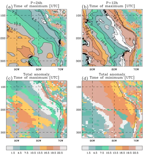
Fig. 7. (a)and(b)Negative phase offset, in hours, of the cosine component of 24-h (left) and 12-h (right) period of the vertical velocity anomalies at 5800 m for the mean diurnal cycle in the SEP.(c)and(d)Approximate time of maximum (positive, left) and time of minimum (negative, right) in the 5800 m vertical wind anomalies. UKMO operational analysis (00:00 h UTC) and forecast (03:00 h–21:00 h UTC) data at three-hourly intervals.

circulation with the march of the season. We focus here on changes in the subtropical jet stream and on diabatically forced streamfunction anomalies that interested the SEP.

The storm-track is markedly different between three me-teorologically distinct periods (discussed in Sect. 7.2) that characterised VOCALS-REx (Fig. 8). In October, upstream of the south-American coast the storm track has a broader meridional spread, with activity at sub-tropical latitudes north of 30◦. A strong interaction with the continental to-pography is suggested by the maxima on the two sides of it. In early November, by contrast, storms develop in a narrow, sub-polar zonal band, with little evidence of affecting the tropical inversion in the way indicated in Fig. 19. Later still,

while baroclinic activity returns north, it appears weak near the South-American coast. This period in the second half of November is also characterised by steady north-westerly mid-tropospheric flow, accompanied by reduced subsidence (Fig. 20c).

Fig. 8. (a), (b), and(c)6-day running standard deviation of the 1-to-6-day high-pass filtered 50 hm streamfunction for three mete-orologically distinct periods during the VOCALS-REx campaign. Data from the UKMO operational analyses.

ascending circulation associated with the equatorward flank of a storm track can have on the Sc inversion.

The changes in the storm track during the two months of the campaign within the SEP sector reflect, at least in part, the normal seasonal evolution of the large-scale circulation. In general, the spring season is characterised by a large shift in the mid-latitude jet. In the south Pacific, the sub-tropical branch weakens considerably, and a characteristic split-jet structure emerges.

This evolution is represented in Fig. 9 for October– November 2008. The subtropical jet, which is prominent during the first half of October, shows a split structure with a distinct sub-polar branch in the second half of the month, and is largely reduced to the Indo-Australian sector in November. This evolution may explain some of the changes observed in baroclinic activity investing the VOCALS-REx region. In

addition, the subtropical jet initially acts as a wave-guide for any disturbances generated upstream, resulting in very weak persistent wave-like anomaly patterns, hardly escaping tropical latitudes. Starting from the beginning of Novem-ber, with the break-down of the subtropical jet, and the in-creased prevalence of (weak) westerlies near the tropical ar-eas of deep convection, a slowly evolving Rossby wave pat-tern begins to appear, which is well established in the last period of the campaign, with increased cyclonic circulation over the SEP, coincident with northerly flow, and dynami-cally induced lofting from vorticity conservation. The occur-rence of this pattern coincides with the increased day-time cloud break-up which characterised the latter part of the cam-paign.

In parallel with this evolution poleward of the VOCALS-REx area, beginning from the last days of October and into the first half of November moist convection over tropical South America becomes active, establishing at least tem-porarily a characteristic (e.g. Fig. 2) warm anticyclone over the Bolivian Altiplano (Fig. 9c), as might be generally ex-pected from the progression of the season. This activity is associated with a particularly warm upper troposphere and increased descent above the VOCALS-REx area during that period. We will see in the next Sect. 6 however that tropical convection over South America was, in general, relatively weak during Spring 2008.

6 Anomalies and teleconnections

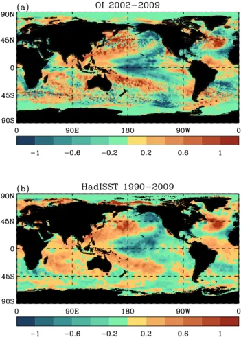
For the duration of the campaign, large-scale SSTs anomalies in the sub-equatorial Pacific indicate a prevalence of weak La-Ni˜na like conditions (Fig. 10). In the eastern Pacific, however, SSTs are close to their climatological values. In-situ and satellite SST products indicate that anomalies in the SEP for October and November 2008 are less than 0.5◦C in magnitude. These values are comparable with the discrep-ancies among such products, and therefore not significant. Among the data-sets used in Fig. 10, the NOAA OI most closely matches the in-situ data collected by the R. H. Brown near 20◦S in November. The UKMO OSTIA product com-pares even better, but it covers an insufficient temporal span for an estimate of the interannual anomaly. Averages for the single months of October and November do not show addi-tional significant features.

Fig. 9. Zonal wind at 200 hPa, in units of m s−1, for four fort-night periods in October and November 2008 (colour coding, scale at the bottom). Contour lines show the zonally asymmet-ric component of the 200 hPa streamfunction. Contour interval is 4×106m2s−1; white contours indicate negative values (clock-wise, or cyclonic, circulation in the Southern Hemisphere), and black positive values (anticlockwise, or anticyclonic, circulation). Data from UKMO operational analyses.

high between October and November is stronger than usual. Conversely, at the sub-tropical latitudes of VOCALS-REx (north of 45◦S), synoptic variability, as estimated from the 7-day high-pass filtered variance of the 500 hPa streamfunc-tion in the ERA-Interim reanalysis, is below the climatolog-ical average for the period 1989–2008, especially in October (not shown). The anomaly resembles that of early November compared to October 2008 (Fig. 8, panels (b) and (a), respec-tively). The implication is that the strong baroclinic activity observed in October to invest the VOCALS-REx area was not by any means exceptional, and the transition to reduced mid-tropospheric synoptic variability probably less marked than normal.

Fig. 10. SST anomalies as diagnosed for the period October– November 2008 as estimated from satellite-derived (NOAA OI v2; panela) and from in-situ (HadISST; panelb) data products. The reference periods used for the climatologies are given in the title of each panel.

Towards the end of the previous section we noted that the upper-level circulation in this period appears to have been mainly remotely forced. Consideration of the interannual anomalies tends to support this hypothesis. Figure 12 shows the interannual anomalies, for the same four periods of Fig. 9, of TOA OLR (green contour lines), velocity potential (colour coding), and eddy streamfunction (white contour lines).

Although the weak warm SST anomalies in the Atlantic might be expected to act to sustain convective activity over the Amazon basin, this was subdued compared to the clima-tology (cf. Fig. 12). Increased, i.e. near-climatological activ-ity between the end of October and the first half of November gave way to a further dry spell, with rainfall moving north of the Equator at the end of the VOCALS-REx period.

Fig. 11.Interannual anomalies for the months of October and November 2008. Panels(a)and(c)show the geopotential height at 500 hPa, panels(b)and(d)the anomalies in sea-level pressure. Reference climatology is for the period 1989–2008. Data from the ERA-Interim reanalysis (Simmons et al., 2006).

velocity-potential and streamfunction anomalies are consis-tent with a quasi-stationary Rossby wave-train emanating from the region of enhanced convection west of the date-line, which generate a Pacific-South-American (PSA) pat-tern, with a cyclonic centre in the SEP, in late November. A connection of this type between convective activity in the West Pacific and the occurrence of a PSA pattern of the sign given in Fig. 12 has been shown in the climatological context by Mo and Higgins (1998). We will see below that the per-sistent cyclonic anomaly over the SEP had significant conse-quences for the regional meteorology observed in VOCALS-REx.

7 Characterisation of the meteorology during VOCALS-REx

7.1 General

Figure 13 depicts the mean surface and MBL conditions en-countered during the VOCALS-REx observations campaign between 1 October and 2 December 2008.

As is typical for austral spring, sea surface temperatures (SSTs) along the coast were cold offshore of the strongest upwelling zones. These are located both to the south and to the north of the Arica bight, where SSTs had a local maxi-mum (Fig. 13b). Away from the coast, the SST gradient is to the west and northwest.

Within the region of observations, surface winds were typically south-southeasterly, with a direction ranging from 177◦at 20◦S, 71◦W to 125◦at 20◦S, 85◦W (Fig. 13a). West of 75◦W, directionality was very steady, with a daily stan-dard deviation of less than 10◦; this figure rises to about 30◦ close to the coast.

Fig. 12.Velocity potential and streamfunction anomalies at 200 hPa (colour-coding and black and white contours, respectively) from ERA-Interim, and OLR anomalies (yellow contours) from the NCEP CDC interpolated OLR data-set, for the four periods corre-sponding to the four panels in Fig. 9. The units for the velocity po-tential are 107m2s−1, and the contour interval is 2×106m2s−1. The streamfunction anomalies are given in units of the local stan-dard deviation from the 20-yr monthly-mean climatology. The con-tour interval is 1.5, with the zero-line omitted, and concon-tours are black for positive, and white for negative values. For OLR, the con-tour interval is 7 W m−2, and contour lines are broken for positive values, and solid for negative values.

or near-saturation to less than 10 %, although higher values have also been observed. A thermal wind is associated with the mean gradient in inversion height. Near 20◦S, the latter is largely aligned with the wind itself, resulting in little direc-tional change (a slight backing), and the wind remains east-ward near the coast and north-easteast-ward offshore. An addi-tional thermal wind component above this level is associated with the predominantly meridional mean temperature

gradi-1014

1016

1018

1020

1022

-85 -80 -75 -70

-85 -80 -75 -70

-30 -25 -20 -15 1024 0.1 0.1 0. 2 0.3 0.3 0.3 0.4 0.6 0.6 0.₆ 0.7 0.₇ 0.8 0.8 0.9 0.₉

-85 -80 -75 -70

-30 -25 -20 -15 surface pressure [hPa] surface 850 hPa Streamlines 10 0

speed [m s-1]

288

289

290

291 292

-85 -80 -75 -85 -80 -75

17 18 19 20 21 22 23 24 24 25 26

-85 -80 -75

LTS [K] Water cloud fraction [MODIS] ~10:30am local Water cloud fraction [MODIS] ~10:30am local (a) (a) (b) (c) (d) 30 4050 50 60 60 60 70 70 70 70 70 80 80 80 80 90 90 90 90 90 90 90 90 100 100 100 100 100 100 100 110 110 110 110 120 120 130 130 130

-85 -80 -75 -70

-30 -25 -20 -15 50 60 70 70 80 90 10 0 110 110 120 120 120 130 130 130 140 150

-85 -80 -75

100 (f) (e) a a a a)) (((a (a 0 0 0 9 0 999 0.0.₉₉₉₉₉₉ 8 0₈ 0₈ 0₈ 0₈ 0₈ 0 0 0 0 8888 0.7 0.7 0000 0. 0. 00₇₇₇₇ 0 0 0.6 0.6 000.6 0.6 77777 0. 0.₆₆₆₆₆ 666 0 .3 0. .3 0. 0

0 44

u u ud ud ud r r rrr W W W W W W W alll o o o d d d d d d d d d d d W W W W Wat Wat Wat Watteteteteerererer Water Water S S S M M M M MOOOOOOOO SSSSSSSSSS MO MO MO MO MO MO o o io ioononononon [nn [n[M[[M[ io io

io MMMM

ion ion ll l l l l l l l l l l o o o o o o o o Cloudy LWP MODIS [g m-2_]

Cloudy LWP AMSR

[g m-2_]

Fig. 13. October–November mean values of(a)sea level pressure (colour contours) and flow streamlines at the surface (black) and at 850 hPa (white);(b)sea-surface temperature from the NOAA Op-timal Interpolation analysis; (c)fractional cover of water clouds for October–November 2008 at 10:30 a.m. local time as deter-mined by MODIS;(d) lower tropospheric stability (LTS, differ-ence between potential temperature at 700 hPa and surface) from the ECMWF operational analyses;(e)mean LWP for cloudy pixels from MODIS;(f)mean LWP for cloudy pixels from AMSR (AMSR LWP/MODIS warm cloud fraction). In(e)and(f), we use the area mean diurnal mean LWP from AMSR (mean of 01:30 and 13:30 LT) divided by the mean warm cloud cover from MODIS, to provide an estimate of the cloudy sky LWP.

The mean liquid-water cloud cover, obtained from MODIS Terra satellite at 10:30 LT, is shown in Fig. 13c. It reaches its maximum within a belt at a distance of 500 km from, and roughly parallel to, the Peruvian coast, with mean values exceeding 90 %. This region is situated a few hundred km downwind of the maximum in lower tropospheric stability (LTS, Fig. 13d), which is defined the difference between the potential temperature at 700 hPa and the surface. Over most of the region sampled in VOCALS-REx the mean warm-cloud cover exceeded 70 %, except very close to the coast where topographic irregularities and the advection of drier air masses are conducive to local clearings.

Figure 13e and f also show the mean liquid water path (LWP), as determined for cloudy pixels using the visible/near-IR retrievals from MODIS (panel e) and from the passive microwave Advanced Microwave Scanning Ra-diometer (AMSR; panel f). The two estimates agree very well within about 500 km of the coast, where the poten-tial contamination of the AMSR estimate by drizzle is lim-ited (as evidenced from VOCALS-REx aircraft observations, Bretherton et al., 2010). Within this region, typical cloud LWP values were 70 g m−2or less.

Liquid water paths increase westwards, in agreement with in-situ observations (Bretherton et al., 2010). Still further west, the microwave-derived LWP estimates from AMSR in-creasingly exceed those from MODIS, which is indicative of increasing amounts of drizzle (see e.g. Shao and Liu, 2004) formed in the thicker clouds of the deeper maritime MBL (Wyant et al., 2010; Zuidema et al., 2009).

While the mean flow illustrated in the previous section is somewhat representative of the observed day-to-day condi-tions in the MBL, in the FT variability on synoptic time-scales was very substantial.

The cloud-cover was observed to respond to the synoptic-scale variability of the circulation above the inversion to a de-gree such that the 48-h operational forecasts of synoptic con-ditions could be usefully employed to estimate the expected changes in observable field conditions during the VOCALS-REx campaign. The forecast cloud fields themselves pro-vided a good guidance for the expected cloud cover.

In general, the main source of synoptic variability in the VOCALS-REx region was baroclinic activity in the jet-stream system, causing ridging and troughing in the FT which tended to be amplified by orographic effects near the Andes. This was associated with anomalous advection of air-masses from different latitudes or altitudes, following the ridging of the isoentropes.

When the disturbance was sufficiently strong, it developed into a coastally-intensified cyclone (Garreaud et al., 2002; Garreaud and Rutllant, 2003), most clearly seen in the lower FT at about 700 hPa. In a few instances (e.g. 19–20 Novem-ber), such coastal lows locally reversed the zonal component of the flow across the Andes to easterly, causing the advec-tion of land air-masses into the maritime SEP area.

While anomalous cold or warm advection in the FT associ-ated with these systems was common, occasionally regions at the low-latitudes of the VOCALS-REx area were directly in-terested by trailing cold fronts, with an ensuing sharp drop in FT temperatures. Such events appear to be more frequent on the eastern slopes in the lee of the Andes, but on 23–24 Oc-tober such a cold front extended throughout the troposphere just above the MBL along 20◦S.

In addition, changes in the extent of the mid-tropospheric high, associated with changes in heating either from the el-evated terrain of the Bolivian altiplano or from deep con-vection on the western and southern Amazon basin, caused modulations of the sub-tropical jet-stream on its equatorward flank which sometimes were associated with the formation of low-latitude cyclones.

7.2 The day-to-day synoptic conditions over the SEP Depth of the MBL and variability in oceanic cloud during October and November 2008

Superimposed on the night time1T fields in Fig. 14c are sea-level pressure contours for the previous 00:00 UTC, and on the day time field contours of the zonally asymmetric part of the 500 hPa geopotential height field are drawn. The final two panels in Fig. 14c show the average night-time and day-time cloud-top temperatures at each location whenever low cloud is diagnosed (i.e. whenever 1T is within the stated thresholds of 6 K and 35 K), with contours for mean pressure and 500 hPa height overlaid as before.

We discuss here two important aspects of the variations in the cloud field in the VOCALS-REx region. Day-to-day vari-ations in the cloud fields are comparable to diurnal varivari-ations, and in some cases dominate. These synoptic changes oc-cur in coincidence with changes in sea-level pressure and the passage of mid-tropospheric synoptic-scale disturbances. In particular, there is a strong association between low 500 hPa heights and cyclonic flow at 500 hPa, and large-scale clearing and breaks in the cloud cover, particular towards the south of the VOCALS-REx study region. This is particularly ev-ident when synoptic systems approach the South American coast (e.g. 1–3 October, 10–13 October, 20–25 October, 12– 15 November, and after 24 November). Equally remark-able are the intervening episodes of synoptic ridging, par-ticularly during October, which coincide with increased Sc cloud-cover.

Superimposed on this distinctly synoptic variability, circulation-related anomalies can be observed at both smaller and larger spatial and temporal scales. Near land, enhanced orographic subsidence associated with synoptic-scale ridging is responsible for sudden, strong coastal clearings.

This is accompanied by a localised reduction in sea-level pressure and formation of a coastal low (CL), as discussed in Garreaud et al. (2002). The coastal clearings typically persist for up to 3 days after the initial mid-tropospheric ridging, and they tend to be located in the southern part of the domain of interest here, where the coastal jet is strongest, consistent with the dynamics discussed by Munoz and Garreaud (2005). Such “canonical” CLs are seen to occur during 4–5 October, 17–18 October, and 10–11 November.

The association between mid-tropospheric ridging and sea-level troughing along the coast distinguishes CLs from mid-latitude synoptic disturbances (Garreaud et al., 2002). Nevertheless, their character is thought to depend princi-pally on the interaction of synoptic-scale disturbances with the mountain topography, whereby changing up- and down-slope flows affect the temperature and moisture stratifica-tion of the lower atmosphere near the coast, thereby affect-ing the pressure field. These changes also affect the cloud-cover. Thus, on the one hand, CLs depend on the presence of large-scale ridging and troughing. On the other hand, height anomalies associated with synoptic disturbances generally tend to assume a baroclinic character as they interact with the orography, and to disturb the coastal cloud field in a way consistent with the associated mountain winds.

Thus, there are instances – such as 1–2 November – of weak coastal troughing and of ridging at 500 hPa height, which are hardly accompanied by sea-level changes, but nonetheless affect the cloud field, sometimes quite signifi-cantly (e.g. 7–9 November). This particular extensive cloud-clearing event is still associated with mid-latitude trough-ing further south (at the southern edge of the VOCALS-REx study region), but also with strong warming of the mid-troposphere overlying the coastal ocean north of about 25◦S, that appears to emanate from the continent to the east. This results in an enhanced mid-tropospheric meridional temper-ature gradient, and strong cold advection over the southern half of the domain (see Fig. 16).

The importance on the regional scale of synoptic ridging and troughing near the coast also concerns the origin of the air-masses, and their accompanying aerosol or pollutant load, that were sampled in the SEP area during the VOCALS-REx campaign. The back-trajectories arriving near the inversion along 20◦S during VOCALS-REx, shown in Fig. 15, high-light two particular episodes during which air-masses were advected towards the Sc closer to the coast (typically, within 5 degree in longitude) from potentially polluted land areas. The first such episode occurs in 17–21 October, following an intense synoptic troughing and subsequent ridging along a NW-SE axis to the south of the VOCALS-REx area. The corresponding turning of the geopotential height contours implies advection from the central and southern portion of the Chilean land-mass. Over 20◦S, the ridging peaks on 17 October and coincides with a shallow MBL and persistent, continuous cloud cover. A weaker, but similar occurrence is seen on 16 November, also corresponding with a depressed MBL and increased cloud-cover along 20◦S. Such episodes roughly represent an intensification of the anticyclonic circu-lation south of the VOCALS-REx area which may be brought about by synoptic ridging.

Fig. 14a. Twice-daily snapshots (UTC time as indicated) of the temperature difference1Tbetween the OSTIA SSTs and the GOES Channel 5 brightness temperature. The gray colours indicate the presence of low clouds, with lighter shades indicative of higher clouds in deeper boundary layers. The contour interval for the shading is 3 K. Values of

1Tbelow 6 K are shown in black, and values above 35 K are shown in white (cf. Fig.14c). See text for full details. The contour lines in the night-time panels show the sea-level

pressure for the previous 00:00 UTC. The contour interval is 1.5 hPa; the 1020 hPa line is drawn in light orange colour, and the 1018.5 hPa line in light cyan. On the day-time panels, contours of the zonally asymmetric part of the 500 hPa geopotential height field are drawn, for the subsequent 00:00 UTC. A contour interval of 15 m is used, with positive values

Fig. 16. (a)Hovm¨uller diagram of lower tropospheric stability (θ700−θsurf; colour-coding) averaged over 80–85◦W, as a function of time and latitude; the black contours show the potential temperature at 500 hPa over the same zonal average.(b)like(a), but for cloud fraction from GOES at 19:28 UTC (late afternoon), shown as black-and-white filling, and 500–700 hPa thickness contours, shown as coloured contour lines. Thickness and temperature data from UKMO global operational analysis and 3 h–21 h forecasts. The abscissa values indicate the day of the VOCALS-REx campaign, with day 1 corresponding with 1 October and day 61 with 30 November 2008.

To some extent, the back-trajectories of air reaching 20◦S between 5 and 7 November highlight the circulation in this mid-tropospheric anticyclone. It is interesting to speculate on the possible role of convection over the Amazon and ad-jacent land. Increased moist convection there and over the Mato Grosso is suggested from satellite OLR maps in the period 18–20 October, and again later between 30 October and 3 November. Such episodic thermal forcing of the mid-troposphere may well excite travelling Rossby waves as sug-gested above. The anomalous upper-level circulation brings tropical, continental air in the vicinity of the MBL in the SEP, in sharp contrast with the usual remote oceanic and subtrop-ical air-mass origin there (cf. Allen et al., 2011). Given the persistent, strong easterly outflow over the low-lying coastal areas of Ecuador, one cannot exclude, in principle, a remote origin from the Amazon basin for some of the air. Con-sidering that South America was anomalously dry compared with climatology (see Fig. 12), and that the events just dis-cussed coincide a period of near-climatological convection, it is possible that air-masses of continental origin over the SEP were anomalously infrequent during the VOCALS-REx campaign.

Dynamical processes at sub-synoptic scales, as discussed e.g. by Munoz and Garreaud (2005), are locally always im-portant near the coast, for example where an approaching

mid-latitude disturbance appears to be associated with the de-velopment of a distinct coastal anomaly ahead of it (e.g. 22– 23 October). Similarly, during 15–16 November, following the passage of a mid-tropospheric cyclone across the Andes, a rapid drop in pressure along the coast coincides with ex-tensive coastal clearing. For reasons both of resolution and imperfect representation of the terrain, this dynamics is not captured by either global or regional forecast models (Wyant et al., 2010; Abel et al., 2010), which all appear to miss the coastal cloud anomalies (along with much of the diurnal cy-cle there). However there is a cy-clear indication from trajecto-ries that become “entangled” with such events that they may considerably prolong the residence time of air-masses above the MBL along 20◦S.

Variability that appears associated with a longer temporal scale is most apparent in the second half of November.

Fig. 17. Inversion height and LCL as estimated from data from R. H. Brown radiosonde launches (black lines), and diagnosed from the UKMO operational forecasts (red lines).

low-pressure centre to the west is part of a slowly evolving wave-train that spans the south-Pacific basin, and appears to emanate from the Maritime Continent, in association with a positive phase of the Madden-Julian Oscillation (MJO), as shown in Sect. 6.

During much of the month of October 2008, changes in cloud cover generally follow a succession of synoptic dis-turbances travelling through the region, with similar effects during the day and during the night. Cloud cover is gener-ally high, with relatively small differences between night and day (in a few instances even negative over the oceanic area west of 82◦W), but is characterised by rapid, near-complete clearing in large, dynamically well-defined areas, dominated by cyclonically turning mid-tropospheric flow, where a com-bination of cold advection and negative-vorticity advection occurs.

Later in the Spring season, from the end of October to the middle of November, diurnal variations in cloud cover are larger, and on sub-synoptic time-scales coastal and other smaller-scale clearing events (such as those associated with pockets of open cells) become more important. During this period, there is little synoptic activity from mid-latitude de-pressions, the cloud cover is nearly complete during night-time, while the day-time break-up, while variable, is never very large, except on 8 November (as discussed above).

As a rough conceptual schematics, one might summarise the previous discussion by dividing the whole of October– November 2008 into three distinct periods. The first period, until the end of October, has robust synoptic activity from mid-latitude depressions which largely control the cloud con-ditions. The second period, in the first half of November, shows reduced baroclinic activity, with high values of

sea-level pressure, and sub-synoptic scale activity, including in-fluences from continental convection, on time-scales of 2– 3 days. The third and final period has moderate synoptic vari-ability, and is dominated by a large-scale circulation anomaly which reduced mid-tropospheric subsidence and allowed for an extensive day-time break-up of the stratocumulus.

Away from the relatively narrow coastal strip, cloud-free areas tend to be zonally aligned and to propagate northwards with the boundary-layer flow. This may be partly due to a memory of the air mass, which being depleted of CCN once a closed to open cell transition involving precipitation occurs (see e.g. 27/28 October case study of Wood et al. (2011) and associated modelling work by Wang et al. (2010) and Berner and Bretherton (2010)), remains so for a length of time. However, at the latitudes most relevant for VOCALS-REx, synoptic disturbances themselves also tend to travel equator-wards as they approach the barrier of the Andes (see Fig. 16).

8 Depth of the MBL and variability in oceanic cloud cover on synoptic time-scales

The operational forecast model of the UK Met Office pro-duces cloud fields which compare well with satellite-derived products in open-ocean areas (Abel et al., 2010, see their Fig. 5). Averaged over the area between 90◦W–80◦W and 15◦S–25◦S, the model-derived daily-average low-cloud cover has a correlation of 0.78 (60 points) with that derived from GOES-10. (An identical correlation is found for av-erages restricted to the zonal strip 90◦W–75◦W, 19.5◦S– 20.5◦S). We also diagnose an MBL-depth from the model fields, by the level of the MBL-capping inversion (the in-version height, hinv). This quantity has a weaker correla-tion of−0.60 with GOES-10 cloud-top brightness tempera-tures. The biggest discrepancies occur in late October and early November, when contamination from cirrus cloud (see Fig. 14c) imply that GOES-10 broad-band IR radiances im-ages do not always reliably represent the Sc top. A good agreement is found between the model-derived hinv and a similarly defined quantity from the profiles returned by ship-based radiosonde ascents (Fig. 17).

Fig. 18. (a)Inversion height from the UKMO forecast model (full black line) and low-cloud cover, all averaged over the region 90◦W– 80◦W, 15◦S–25◦S. The fractional cloud-cover data are shown in violet for the global forecast model, in blue for the limited-area forecast model, and in magenta for the satellite estimates. The thin broken lines show the satellite-derived cloud-cover at 10:28 UTC and 19:28 UTC, respectively; the thicker magenta line is the average.(b)and(c)Composites of inversion height and cloud cover in the region 90◦W–80◦W, 15◦S–25◦S based on the extrema of the daily-average MBL depth. Colours denote the same quantities as in panel(a).

Figure 18 also highlights the different character of the three periods identified in the previous section. Until the end of October, cloud-top heights are very variable, with charac-teristic synoptic temporal and spatial scales. The early part of November, up to the 15th, is generally characterised by low cloud-top heights, especially towards the end; while the second half of November sees higher cloud-tops, prone to day-time break-up. The averages in the area 90◦W–75◦W, 19◦S–21◦S are 1569 m, 1461 m, and 1587 m forhinvfor the periods 1–31 October, 1–15 November and 16–30 Novem-ber, respectively. Correspondingly, the model-derived frac-tional cloud cover is 0.72, 0.80 and 0.60, respectively; the

The UKMO operational model has no representation of cloud-aerosol interaction, and a very rudimentary parametri-sation of cloud-microphysical effects. Moreover, its horizon-tal resolution cannot capture the effect of precipitation on mesoscale dynamics in the MBL. The model does not have any representation of mesoscale or smaller features, includ-ing for example the development of pockets of open cells. Thus, its qualitative consistency with observations in both MBL-depth and cloud-cover is non-trivial. Although the model tends to dissipate some cloud with increasing forecast lead time, the simulated day-to-day variability is not solely or primarily due to assimilation increments. Initialised free-running simulations of the model in one of its climate config-urations, HiGAM (Shaffrey et al., 2009), show an evolution of the cloud field in the SEP that remains very close to the op-erational analyses for up to 10 days. Therefore, the UKMO operational forecasts represent a valuable opportunity to iso-late the effects of dynamical forcing on the Sc field in the VOCALS-REx region.

In this model, an elevated inversion consistently corre-sponds with increased area cloud fraction if averages over a sufficiently large area and away from land are considered. Figure 18 highlights variability with a typical synoptic time-scale of about a week or less. However, over the observations period there is no clear indication that this correlation breaks down on longer time-scales. Smoothing the two time-series in Fig. 18 still results in formally significant correlations. Nevertheless, it appears that large-scale circulation anoma-lies not associated with synoptic-scale systems, which af-fected VOCALS-REx in the second half of November, when cloud cover was considerably reduced, do play a role. It is apparent, also, that especially intense synoptic events, such as that occurring in 22–24 October, are more than proportion-ally effective in reducing cloud cover, leaving a signature on longer time-averages. This acquires particular significance when considering that, because of the day-time cloud break-up, the relationship between cloud cover and surface insola-tion is also skewed in the same sense.

Figure 19 shows the mid-tropospheric circulation anoma-lies associated with changes in the inversion height in the area 90◦W–75◦W, 19.5◦S–21.5◦S (indicated by the black rectangle). The composites based on the inversion height (hinv) extrema of Fig. 18 indicate that negative (positive) inversion-height anomalies (with positive/negative cloud-cover anomalies) coincide with anomalous warm (cold) ad-vection in the FT within anticyclonic (cyclonic) synoptic dis-turbances when they approach the area of interest. Vertical sections in the meridional plane of these events (not shown) confirm a baroclinic structure, with descent (ascent) associ-ated with a tilted warm (cold) front. Linear correlations with

hinv (not shown) show a very similar, formally significant structure. As may be expected, the associated temperature advection is most intense in the lower free-troposphere just above the MBL.

Fig. 19. Composite maps of 50 hm streamfunction anomalies and vertically integrated temperature advection in the FT above the MBL for the positive (panela) and negative (panel b) extremes in inversion height,hinv, shown in Fig. 18. The maps show av-erage anomalies over 48 h prior to the extrema inh_inv. Colour-coding refers to heat advection (units are J m−2s−1; 100 J m−2s−1 roughly correspond to 1 K day−1 mass-averaged anomalous tem-perature tendency in the FT). Coutour lines show the streamfunc-tion anomalies, in units of Mm2day−1. Positive values, marked by black contours, correspond to anticyclonic circulation (apparent in panelb), and negative values for cyclonic circulation. Data from operational analyses and 3 h–21 h forecasts are used.

suggest anomalous ascent near the Andean topography asso-ciated with synoptic troughing, and anomalous descent as-sociated with synoptic ridging. Note also the association of the latter with advection towards 20◦S from land areas to the South (cf. discussion on Fig. 15 in the previous sec-tion). These results are consistent with the analysis of Xu et al. (2005) who find that anticyclonic circulation anoma-lies which tend to reinforce the climatological zonal pressure gradient and generate offshore flow in the lower troposphere off the Chilean coast tend to increase cloud-cover while de-pressing the inversion and represent an important mechanism in the generation of subseasonal variability in the Sc deck. Painemal and Zuidema (2009) find a similar circulation sig-nature from the cloud droplet-number concentrations with anomalous easterly, offshore flow. In our composites the an-ticyclonic anomalies also appear to have a more stationary character than the rapidly evolving cyclones, while the latter are associated with the largest vertical wind anomalies.

In general, the height tendencies may be decomposed into a part due to vertical advection, a part due to horizontal ad-vection, and a part due to entrainment, the latter being diag-nosed as a residual according to

˙

mǫ/ρ=∂thinv+u· ∇2hinv−w, (1)

where all quantities are calculated for z=hinv. Here, m˙ǫ

represent the entrainment flux, u the horizontal wind, and

wthe vertical wind. This decomposition, shown in the thin lines in Fig. 20, shows a dominant contribution for the in-version height tendencies the area 19.5◦S–20.5◦S,90◦W– 80◦W by the horizontal advection of height anomalies in the first period of the campaign (1 October to 27 October), to be later partly replaced by a contribution from vertical velocity anomalies. These results are consistent with those of Rahn and Garreaud (2010b), who perform a similar analysis, and demonstrate that horizontal advection gives the leading-order contribution to changes of the MBL depth over synoptic time-scales. As a comparison with Fig. 19 suggests, we find that vertical advection anomalies become markedly more im-portant near the coast, especially to the South, i.e. upstream, of 20◦S. Thus, temperature anomalies in the lower free-troposphere that are generated by the interaction of synoptic systems with the orography are communicated downstream via horizontal advection.

In general, atmospheric heat advection is dominated by the vertical and meridional components, which partially counter-act each other. Panel (b) in Fig. 20 highlights the dynamical relationship between vertical velocity anomalies and anoma-lies of the meridional flow. Initially, a sequence of upper-level wave cyclones invest the area, with mid-tropospheric ascent and descent associated with poleward and equator-ward flow, respectively. On 22 October, a mature baroclinic system marks the transition to a period with reduced synoptic variability but marked activity by baroclinic planetary waves, in which vertical motion is more strongly associated with the

Fig. 20. (a)Time evolution of the 90◦W–80◦W, 20.5◦S–19.5◦S average inversion height (solid line), compared with the evolu-tion implied by the partial tendencies associated with changes in the vertical velocity only (red line), in horizontal advection only (blue line), and in the residual, interpreted as entrainment (green line). The time-mean values of the partial tendencies were re-moved.(b)Height-time Hovmueller diagram for the 90◦W–80◦W, 20.5◦S–19.5◦S area average meridional (contour lines) and verti-cal (colour-coding) mass-flux for October–November 2008. Con-tour interval is 0.5 kg m−2s−1for the meridional component, and 0.5 g m−2s−1for the vertical component (the transition from cyan to yellow marks the zero line). The height of the inversion is in-dicated by the dark-red line, the excursions from the mean being exaggerated 3-fold for clarity. A 2-day smoothing is applied to all quantities. Data are from the operational analyses for the inversion heightnpanel(a), and from both analyses and 3 h–21 h forecasts for all other quantities.

conservation of potential vorticity. At the level of the in-version, the different character of the evolution between the three periods is seen clearly in panel (b) of the Figure. In early November, the induced motion is downward, to switch to anomalous ascent later.