DOI:10.2298/YUJOR0901157G
A DUAL EXTERIOR POINT SIMPLEX TYPE ALGORITHM
FOR THE MINIMUM COST NETWORK FLOW PROBLEM
George GERANIS
Konstantinos PAPARIZZOS
Angelo SIFALERAS
Department of Applied Informatics, University of Macedonia, geranis,paparriz,[email protected]
Received: December 2007 / Accepted: May 2009
Abstract: A new dual simplex type algorithm for the Minimum Cost Network Flow Problem (MCNFP) is presented. The proposed algorithm belongs to a special “exterior-point simplex type” category. Similarly to the classical network dual simplex algorithm (NDSA), this algorithm starts with a dual feasible tree-solution and reduces the primal infeasibility, iteration by iteration. However, contrary to the NDSA, the new algorithm does not always maintain a dual feasible solution. Instead, the new algorithm might reach a basic point (tree-solution) outside the dual feasible area (exterior point - dual infeasible tree).
Keywords: Operations research, combinatorial optimization, minimum cost network flow problem.
1. INTRODUCTION
The MCNFP can be easily transformed into a Linear Programming Problem and well known general linear programming techniques could be applied in order to find an optimal solution. Such techniques do not take advantage of some special features met in the MCNFP. So, other special Simplex-type algorithms have been developed, such as the Primal Network Simplex Method and the Dual Network Simplex Method. There are also other non Simplex-type algorithms that can be used for the solving of the same problem, as presented in [7], [2] and [15]. An exterior-point primal simplex-type algorithm for solving the MCNFP has also been presented in [13].
This paper comes to present for the first time an exterior point dual simplex-type algorithm for the MCNFP. The algorithm is named Dual Network Exterior Point Simplex Algorithm (DNEPSA) for the MCNFP. It starts with a dual feasible tree-solution and, iteration by iteration, it produces new tree-solutions closer to an optimal solution, reducing the problem’s infeasibility. Contrary to the Network Dual Simplex Algorithm, the tree-solution at every iteration is not necessarily dual feasible but, after a number of iterations, the algorithm reaches a tree-solution that is both primal feasible and dual feasible and therefore it is optimal.
Section 2 gives the notation that will be used in this paper and a short description of the MCNFP. In Section 3, the Dual Network Exterior Point Simplex Algorithm (DNEPSA) is described and the steps that have to be followed are described in detail. An illustrative example presenting the algorithm step by step is given in Section 4. Finally, Section 5 gives some conclusions and plans for future work.
2. NOTATIONS AND PROBLEM STATEMENT
In this Section we shall give a short description of the MCNFP. Let G=(N,A) be a directed network that consists of a finite set of nodes N and a finite set of directed arcs A, that link together pairs of nodes. Let n and m be the number of nodes and arcs respectively. For each node i∈N, there is an associated variable bi representing the
available supply or demand at that node. A node i is a supply node (source), if it is 0
i
b > . On the other hand, it is a demand node (sink), if it is bi <0 . Finally, the node i is a transshipment node in case it is bi =0. The total supply has to be equal to the total demand, i.e. it has to be i 0
i N
b
∈ =
∑
(balanced network).For every arc (i,j) we have an associated flow xij that shows the amount of
product units transferred from node i to node j and an associated cost per unit value xij.
Therefore, the total cost is equal to ( , )
ij ij i j A
c x ∈
∑
and the MCNFP is the problem of finding a flow that minimizes that total cost.We can have, for the flow
x
ij on arc (i,j), a lower and an upper bound, lij andij
u respectively. This gives an additional constraint lij ≤xij≤uij for every arc (i,j). In our
case we consider it is lij=0 and uij = +∞. In other words, our algorithm is applied to the
( , ) ( , )
ij ji i i j A j i A
x x b
∈ ∈
− =
∑
∑
because the outgoing flow must be equal to the incoming flow plus the node’s supply. Therefore, the MCNFP can be formulated as follows:
minimize ( , )
ij ij i j A
c x ∈
∑
(2.1)subject to
( , ) ( , )
ij ji i i j A j i A
x x b i N
∈ ∈
− = ∀ ∈
∑
∑
(2.2)0, ( )
ij
x ≥ ∀ij ∈A (2.3)
Since it is i 0
i N
b ∈
=
∑
, by using formula (2.2), it comes out that( , ) ( , )
( ij ji) 0
i N i j A j i A
x x
∈ ∈ ∈
− =
∑ ∑
∑
That means that constraints (2.2) are linearly dependent and we could arbitrarily drop out one of them. Of course, a problem like this could be solved using standard well-known Linear Programming algorithms, but these algorithms do not take advantage of some special features met in the MCNFP.
There is a set of dual variables wi, one for every node, and a number of reduced
cost variables wij, one for every directed arc. These are the variables used for the formulation of the dual problem. Network simplex-type algorithms start from a basic tree-solution and compute vectors x, w, s consisting of variables xij, w and wij
respectively. If for a tree-solution T, it is xij ≥0 for every arc ( , )i j ∈T, then that solution is said to be primal feasible. If for a tree-solution T, it is sij≥0 for every arc ( , )i j ∉T then it is said to be dual feasible. A solution being both primal feasible and dual feasible represents an optimal solution. Primal network simplex-type algorithms start from a primal feasible solution, while dual network simplex-type algorithms, like the algorithm described here, start from a dual feasible solution.
3. ALGORITHM DESCRIPTION
There are different techniques that can be used in order to find a starting dual feasible tree-solution. An algorithm that can construct a dual feasible tree-solution for the generalized network problem (and also for pure networks) is described in [8] and an improved version of the algorithm is presented in [11], which gives a dual feasible solution that is closer to an optimal solution.
Given the starting dual feasible tree-solution, it is easy, starting from the leaf nodes, to compute the flows xij for all the basic arcs (i,j) in that tree (step 1). It is also
very easy to compute values for the dual variables wi from the equations:
i i ij
w −w =c , for every arc ( , )i j ∈T (3.1)
In equations (3.1) we have n-1 equations and n variables, so, we can choose one of the dual variables (e.g. wi) and set it equal to an arbitrary value (e.g. 0). Then, it is
easy to compute the values of the rest of the dual variables.
In order to calculate the reduced costs sij for the non-basic arcs (i,j), we can use
the following equations:
ij ij i j
s =c +w −w
, for every arc
( , )i j ∉T(3.2)
while it is sij=0 for all the basic arcs.
Next, the algorithm creates a set, named I_, that contains the basic arcs (i,j) having negative flow, i.e. it is xij<0. It also creates set I+ containing the rest of the arcs.
If it is I_=∅, this means that the tree-solution is feasible and therefore it is optimal (step 2).
After this, the algorithm considers the non-basic arcs ( , )i j ∉T . When such an arc (i,j) is added to the basic tree-solution T, then a cycle C is created. That cycle may contain arcs of I_ having the same orientation as (i,j) and others having the opposite orientation. For every non-basic arc, let dij be the difference between the number of arcs
in I_ having the same orientation in cycle as (i,j) minus the number of them having the opposite orientation. J_ consists of those non-basic arcs (i,j) having dij >0 (step 3).
After creating set J_, we have to choose amongst its arcs, the one that will be the entering arc (g,h). This is the arc of J_ that gives the minimum ratio –sij/dij (step 4).
Next, the algorithm has to find the leaving arc (k,l). This is done by checking the cycle C formed after adding the entering arc (g,h) to the tree T. For the arcs of I_ having the same orientation in C as (g,h), we choose arc (k1,l1) that corresponds to the minimum
absolute flow. Similarly, for the arcs of I+ having orientation opposite to the entering arc
(g,h), we choose arc (k2,l2) that corresponds to the minimum absolute flow. If we denote
1
θ and θ2 these two minimum values, we decide the leaving arc by comparing θ1 against θ2. If it is θ θ1≤ 2, then the leaving arc is (k,l) = (k1,l1), otherwise it is (k,l) =
(k2,l2).
The algorithm’s steps are described below. The symbols ↑↑ and ↑↓ used here, denote arcs that have the same orientation or opposite orientation, respectively.
Algorithm DNEPSA
1. Start with a dual feasible tree T. Compute the flow variables xij for all the basic arcs, the dual variables wi and the reduced cost variables sij, by applying formulas (3.1) and (3.2).
2. Set I_=
{
( , )i j ∈T x: ij <0}
and I+ ={
( , )i j ∈T x: ij≥0}
If it is _I = ∅,then the current tree-solution T is an optimal solution. 3. Set
{
}
_ ( , ) : , , ij ij ij 0
J = i j ∉T if added to T in the cycle created it is d = p −n > where pij is the number of arcs in _I having the same orientation as (i,j)
and nij is the number of arcs in _I having the opposite orientation.
4. Choose arc ( , )g h ∈J_, where it is
min{ : ( , ) J_}
gh ij
gh ij
s s
i j
d d
− = − ∈
Arc (g,h) is the entering arc.
5. Compute values θ1 and θ2 where:
{
}
1 1
1 xk l min xi j ( , )i j I_and i j( , ) ( , )g h
θ = = − ∈ ↑↑
{
}
2 2
2 xk l min xi j ( , )i j I and i j( , ) ( , )g h
θ = = − ∈ + ↑↓
If θ θ1≤ 2 then the leaving arc is ( ,1)k =( 1)k , otherwise the leaving arc is
2 2
( ,1)k =( ,1 )k .
6. For the new tree-solution T, compute the flows xi j and the dual problem
variables wi and sij. Repeat the process from step 2.
4. AN ILLUSTRATIVE EXAMPLE
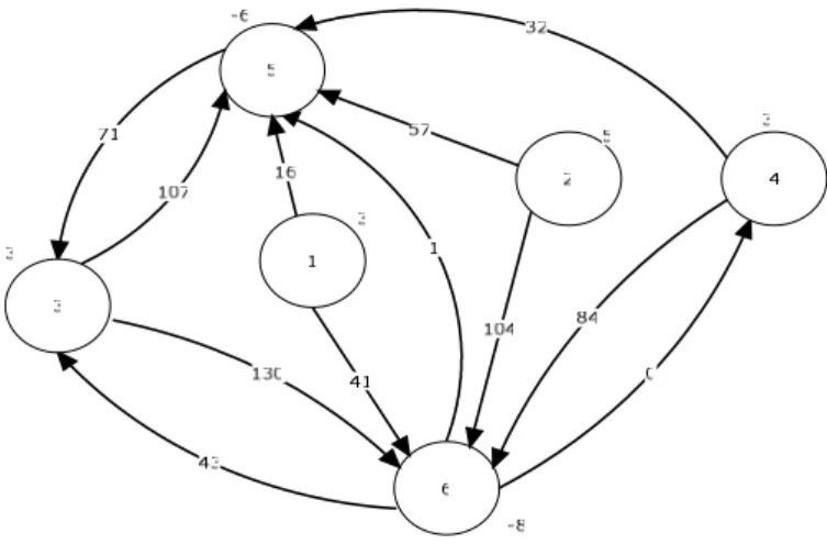
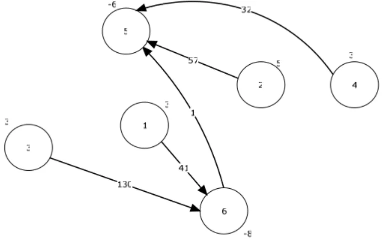
We’ll now give an illustrative, step by step, example where the algorithm presented will be applied to a MCNFP. Figure 1 shows a network G = (N, A), consisting of 6 nodes and 12 arcs. Next to each node there is a value showing the node’s supply (negative values mean demands). For every arc in A, the cost per product unit flow is also shown.
Figure 4.1: The graph G = (N,A) where DNEPSA is applied
We will apply below the algorithm’s steps to find a solution for the MCNFP as applied to graph G. The algorithm finds an optimal solution after 3 iterations.
Iteration 1
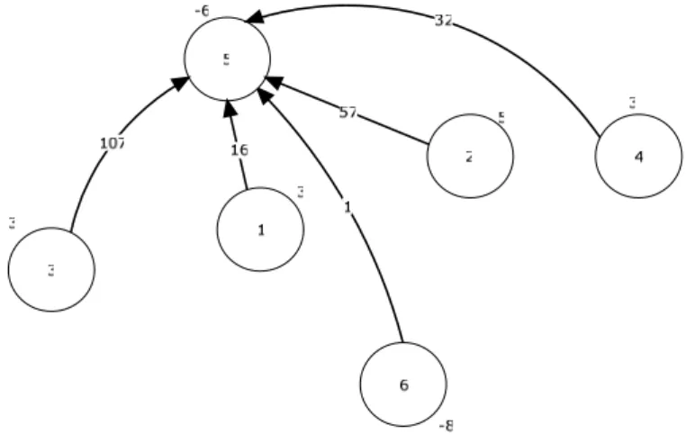
Figure 4.2: The initial dual feasible tree
The tree shown is a dual feasible tree, since it is sij≥0 for every arc (i,j). This can be easily verified by solving equations (3.1), which take the following form:
5 1 16
w −w =
5 2 57
w −w =
5 3 107
w −w =
5 4 32
w −w =
5 6 1
w −w =
By setting w1 equal to 0, we have w5 =16, w2 = −41, w3 = −91, w4 = −16 and
6 15
w = . By applying equations (3.2) we have:
16 16 1 6 41 0 15 26
s =c +w −w = + − =
26 26 2 6 104 ( 41) 15 48
s =c +w −w = + − − =
36 36 3 6 130 ( 91) 15 24
s =c +w −w = + − − =
46 46 4 6 84 ( 16) 15 53
s =c +w −w = + − − =
53 53 5 3 71 16 ( 91) 178
s =c +w −w = + − − =
64 64 6 4 0 15 ( 16) 31
s =c +w −w = + − − =
63 63 6 3 43 15 ( 91) 149
s =c +w −w = + − − =
For every node i in the graph, it is
( , ) ( , )
ik ji i
i k N j i N
x x b
∈ ∈
− =
∑
∑
This happens because for every node the outgoing flow has to be equal to the incoming flow plus the node’s supply. That is, the following equations have to be satisfied:
15
1: 3
node x =
25
2 : 5
node x =
35
3 : 3
node x =
45
4 : 3
node x =
45
4 : 3
node x =
15 25 35 45 65
5 : 6
node −x −x −x −x −x = −
65
6 : 8
node x = −
By solving the above equations we have x15=3
,
x25=5 x45=3 x65 = −8. This is not a feasible tree since we found some negative flows (it is x65<0)Step-2 It is I_ = {(6,5)}, since it is x65= − <8 0 and the remaining arcs form I+.
Step-3 If we add the non-basic arc (1,6) to the basic tree, a cycle C is created. In this cycle, arc (1,6) has the same orientation as (6,5) which belongs to I_. So, (1,6) ∈ J_. By checking in a similar way all the non-basic arcs, it comes out that J_ = {(1,6),(2,6),(3,6),(4,6)} with d16 =d26=d36=d46 =1.
Step-4 For the arcs in J_ it is s16=26, s26=48, s36=48, and s46=53. It is
36
36
24 26 48 24 53
min{ , , , }
1 1 1 1 1
s
d = =
So arc (g,h)=(3,6) is the entering arc.
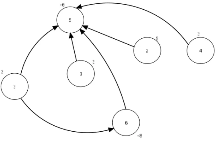
Figure 4.3: The cycle created after adding the entering arc
Arc (6,5) belongs to I_ and has the same orientation as the entering arc (3,6). So, it is θ1 = −x65=8. Arc (3,5), on the other hand, belongs to I+ and does not have the same
orientation as the entering arc. So, it is θ2 =x35=3. We have θ1>θ2 which means that arc (3,5) is the leaving arc.
Step-6 The tree shown in Figure 4 is now the new basic tree.
For the new tree it is x15=3, x25=5, x36=3
, x
36 = 3, x45=3 and x65= −5. This is not a feasible tree, so the process has to be continued. By using formulas (3.1) and (3.2), the same way as for the starting basic tree, we find that s16=26, s26=48,35 24
s = − , s46=53
,
s53=202, s64=31 and s63=173. This new basic tree is not a dual feasible tree-solution.Iteration 2
Step-2 It is I_ = {(6,5)}, since it is x65 = -5 < 0 and the remaining arcs form I+.
Step-3 By checking, as in the first iteration, what happens when the non-basic arcs are added to the basic tree and their orientation, we find that it is J_={(1,6),(2,6),(4,6),(5,3)} withd16 =d26=d46=d53=1.
Step-4 For the arcs in J_ it is s16=26,s26 =48,s46 =53and s53=202. It is
16
16
26 26 48 53 202
min{ , , , }
1 1 1 1 1
s
d = =
So arc (g,h)=(1,6) is the entering arc.
Step-5 After adding the entering arc (1,6) to the tree, a cycle C is created as shown in Figure 5.
Figure 4.5: The basic tree after adding the entering arc
Arc (6,5) belongs to I_ and has the same orientation as the entering arc (1,6). So, it is θ1 = −x65=5. Arc (1,5), on the other hand, belongs to I+ and does not have the same
orientation as the entering arc. So, it is θ2 =x15=3. We have θ1>θ2 so, arc (1,5) is the leaving arc.
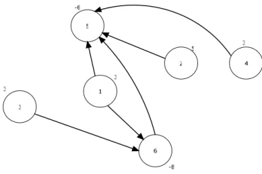
Figure 4.6: The new basic tree-solution
For the new tree, it is x16=3,x25=5,x36=3,x45=3and x65= −2 i.e. it is not a feasible tree. It is also:
15 26, 26 48, 35 24, 46 53, 53 202, 64 31 63 173
s = − s = s = − s = s = s = and s = .
Iteration 3
Step-2 It is I_ = {(6,5)}, since it is x65= − <2 0 and I+ contains the remaining arcs.
Step-3 Similarly, as in the previous iterations, we find that J_={(2,6),(4,6),(5,3)} and
26 46 53 1
d =d =d = .
Step-4 For the arcs in J_ it is s26=48,s46=53and s53=202. It is
26
26
48 48 53 202
min{ , , }
1 1 1 1
s
d = =
So, arc (g,h)=(2,6) is the entering arc.
Figure 4.7: The basic tree after adding the entering arc
Arc (6,5) belongs to I_ and has the same orientation as the entering arc (2,6). So, it is θ1= −x65=2. Arc (2,5), on the other hand, belongs to I+ and does not have the same
orientation as the entering arc. So it is θ2 =x25=5. It is θ θ1≤ 2 so arc (6,5) is the leaving arc.
Step-6 Therefore, the new tree shown in Figure 8 is now the basic tree.
Figure 4.8: The new basic tree-solution
For this tree it is x16=3,x36=3,x45 =3,x26=2and x25=3, i.e. it is a primal feasible tree-solution and also a dual feasible tree since it is
15 22, 35 24, 46 5, 53 154, 64 79, 65 48 63 173
found an optimal solution. This is detected immediately by our algorithm since it is _
Ι = ∅ and the algorithm stops.
5. CONCLUSIONS AND FUTURE WORK
First of all, we plan to present all the necessary mathematical proof of correctness of the proposed algorithm in a future work. DNEPSA is based on a set of lemmas and theorems, which were omitted in this paper, due to paper length. Furthermore, there are special improved data structures that could be used in order to improve the performance of DNEPSA. Such data structures include dynamic trees and Fibonacci heaps, as described in [10], [16] and [6]. There are also other useful data structures and techniques, as presented in [3] and [5], which obtain very good performance, by applying various operations on graphs and trees.
There are several state-of-the-art algorithm implementations that can be applied to the MCNFP. For example, implementations like RELAX IV, NETFLO and MOSEK demonstrate very good performance results. Some of these implementations are described in [4] and [14]. At this point, DNEPSA has already been developed (in C programming language) and tested thoroughly against a big variety of problems. Therefore, it will be very interesting to compare DNEPSA against some of the well known MCNF algorithms
Finally, DNEPSA will be incorporated into the Network Optimization suite WebNetPro which is described in [13]. This way, WebNetPro’s capabilities will be extended by adding new algorithms into this web suite.
REFERENCES
[1] Ahuja, R., Magnanti, T., Orlin, J., and Reddy, M., “Applications of network optimization”, Handbooks of Operations Research and Management Science, (1995) 1-83.
[2] Ahuja, R., and Orlin, J., “Improved primal simplex algorithms for shortest path, assignment and minimum cost flow problems”, Massachusetts Institute of Technology, Operations Research Center, Massachusetts Institute of Technology, Operations Research Center, Working Paper OR 189-88, (1988).
[3] Ali, A.I., Helgason, R.V., Kennington, J.L., and Lall, H.S., “Primal simplex network codes: State-of-the-art implementation technology”, Networks, 8 (4) (1978) 315-339.
[4] Bertsekas, D. P., and Tseng, P., “RELAX-IV: A Faster version of the RELAX code for solving minimum cost flow problems”, Technical Report, Massachusetts Institute of Technology, Laboratory for Information and Decision Systems,1994.
[5] Eppstein, D., “Clustering for faster network simplex pivots”, Proceedings of the 5th Annual
ACM-SIAM Symposium on Discrete Algorithms, 1994.
[6] Fredman, M., and Tarjan, R., “Fibonacci heaps and their uses in improved network optimization algorithms”, Journal of the ACM, 34 (3) (1987) 596-615.
[7] Glover, F., Karney, D., and Klingman, D., “Implementation and computational comparisons of primal, dual and primal-dual computer codes for minimum cost network flow problems”, Networks, 4 (3) (1974) 191-212.
[8] Glover, F., Klingman, D., and Napier, A., “Basic dual feasible solutions for a class of generalized networks”, Operations Research, 20 (1)(1972) 126-136.
[10] Goldberg, A., Grigoriadis, M., and Tarjan, R., “Use of dynamic trees in a network simplex algorithm for the maximum flow problem”, Mathematical Programming, 50 (3) (1991) 277-290.
[11] Hultz, J., and Klingman, D., “An advanced dual basic feasible solution for a class of capacitated generalized networks”, Operations Research, 24 (2)(1976).
[12] Karagiannis, P., Markelis, I., Paparrizos, K., Samaras, N., and Sifaleras, A., "E - learning technologies: employing matlab web server to facilitate the education of mathematical programming", International Journal of Mathematical Education in Science and Technology, Taylor & Francis Publications, 37 (7) (2006) 765-782.
[13] Karagiannis, P., Paparrizos, K., Samaras, N., and Sifaleras, A., “A new simplex type algorithm for the minimum cost network flow problem”, Proceedings of the 7th Balkan Conference on Operational Research, 2005, 133-139.
[14] Kennington, J.L., and Helgason, R.V., Algorithms for Network Programming, Wiley Publications,1980.
[15] Orlin, J., “Genuinely polynomial simplex and non-simplex algorithms for the minimum cost flow problem”, Sloan School of Management, M.I.T., Cambridge, MA,Technical Report No. 1615-84, 1984.