Vol 19 (2009), Number 1, 123-132 DOI:10.2298/YUJOR0901123S
A PRIMAL-DUAL EXTERIOR POINT ALGORITHM FOR
LINEAR PROGRAMMING PROBLEMS
Nikolaos SAMARAS
Angelo SIFELARAS
Charalampos TRIANTAFYLLIDIS
Department of Applied Informatics, University of Macedonia Greece, Thessaloniki
samaras,sifalera,[email protected]
Received: December 2007 / Accepted: June 2009
Abstract: The aim of this paper is to present a new simplex type algorithm for the Linear Programming Problem. The Primal - Dual method is a Simplex - type pivoting algorithm that generates two paths in order to converge to the optimal solution. The first path is primal feasible while the second one is dual feasible for the original problem. Specifically, we use a three-phase-implementation. The first two phases construct the required primal and dual feasible solutions, using the Primal Simplex algorithm. Finally, in the third phase the Primal - Dual algorithm is applied. Moreover, a computational study has been carried out, using randomly generated sparse optimal linear problems, to compare its computational efficiency with the Primal Simplex algorithm and also with MATLAB’s Interior Point Method implementation. The algorithm appears to be very promising since it clearly shows its superiority to the Primal Simplex algorithm as well as its robustness over the IPM algorithm.
Keywords: Linear optimization, simplex-type algorithms, primal-dual exterior point algorithm, computational study.
1. INTRODUCTION
feasible basis and uses pivot operations in order to preserve the feasibility of the basis and guarantee monotonicity of the objective value.
Many pivot rules are known for simplex type algorithms. Much recent research around linear programming algorithms aims to efficiently combine both primal and dual paths thus reducing the duality gap and converging to the optimal solution faster. It is well known that simplex type algorithms behavior can be improved by modifying: (i) the initial solution and (ii) the pivoting rule. A relative new idea is to combine interior point methods and pivoting algorithms for solving linear programming problems [5]. This paper takes advantage of the new primal potential – dual exterior point algorithm [6], [8], [9] and [10], by employing a totally new-in-way constructive implementation. Primal-Dual exterior point algorithm traverses across the interior of the feasible region in an attempt to avoid the combinatorial complexities of vertex-following algorithms. In this paper, we will examine in detail the construction of an initial primal and dual basis, required to initialize the algorithm, along with a computational study to examine its practical effectiveness versus some well known linear programming algorithms.
The paper is organized as follows. In Section 2 we have presented a new method for acquiring the pair of primal and dual solutions; both of which need to start with the algorithm. In Section 3 we have described the primal-dual algorithm. In Sections 4 and 5 we have presented the implementation techniques and the computational results and finally, in Section 6 we have given our conclusions.
2. ALGORITHM INITIALIZATION
The proposed algorithm is directly applied to the primal problem. However, the first step is to obtain a set of primal and dual solutions for this primal problem. The linear optimization problem, in standard form, is as follows:
min subject to 0.
T c x Ax b x
= ≥
(LP. 1)
, mxn , n, m where A∈\ c x∈\ b∈\ .
The corresponding problem to the primal dual one is shown below:
max subject to 0.
T
T
b y
A y z c
z
+ = ≥
(DP. 1)
, m where y z∈\
2.1 Constructing a primal feasible solution
Primal means that this solution refers to the primal problem and not the dual one. Such a requirement is easy to implement using a modified problem with one artificial variable. This problem is capable of providing an initial primal feasible partition by giving priority to the artificial variable to leave the basis. Meanwhile this problem has always an initial feasible algorithm solution applicable by its own unique and strictly constructive format.
As so, by applying primal Simplex algorithm to this modified problem, due to the fact that this algorithm constructs finite sequences of feasible basic partitions, this solution will remain feasible after the artificial variable leaves the basis. There is also the case that the artificial variable has not yet left the basis but the problem has already been solved. A careful pivot should then be able to remove the artificial variable. The modified problem of Phase I is constructed following the procedure below:
We insert the artificial variable xn+1 to our initial linear problem as an extra column in matrix A which is:
B d = −A e
where e is a column vector of ones, having as many rows as matrix A does. The problem which is solved in Phase I is as follows:
1 1 1 min subject to , 0. n n n x
Ax dx b
x x + + + + = ≥
(LP. 2)
A pivot must now be done in order to enter the artificial variable to the basis. The leaving variable is selected by the following minimum ratio test:
( ) min{ ( ) : 1, 2,..., }
k B r B i
x =x = x i= m
The new basic partition is: { } { 1}
{ 1} { }
B B k n
N N n k
← ∼ ∪ +
← ∼ + ∪
The pivoting column which corresponds to the artificial variable is:
1
1 .( 1)
n n
h+ =B A− +
The above selections of entering and leaving variables, assures the feasibility of the first partition in order to apply the primal Simplex algorithm to (LP. 2). This procedure provides us the initial feasible point y for PDTPSA. We can also detect infeasibility through the criterion xn+1>0.
2.2 Constructing a dual feasible solution
min subject to , 0.
T
c x Ax s b x s
+ = ≥
(LP. 3)
We will now formulate a second modified problem which differs from the original as shown below:
min
subject to 0 , 0. T c x Ax s x s + = ≥
(LP. 4)
It can be observed that the right hand side is zero. This gives us the ability to apply the Simplex algorithm from the beginning because the initial partition will be feasible:
1
0 0
B
x =B b− = ≥
This problem has the same solution type as the original one. If the original is optimal, or unbounded this one is also optimal or unbounded correspondingly. This is because the existence or non-existence of optimal points in functions, is not affected by the existence of constant terms. This problem is also not infeasible because the trivial solution x = 0 always exists. Regardless, we must construct this modified problem only if Phase I has proved that our original problem is not infeasible. In any case (LP. 4) is either optimal or unbounded. If it is optimal, its optimal partition is also dual feasible to (LP. 3) because the right hand side does not participate in the computation of the dual slack variables, and so remains the same for the pair of problems. On the other hand in case the problem is unbounded, then (LP. 3) is unbounded also, because such a system remains so regardless of its right hand side.
3. ALGORITHM DESCRIPTION
The algorithm geometrically moves from an exterior dual feasible point towards the interior of the feasible region using either a boundary or an interior starting point. If an interior point is used then the direction drawn crosses the polyhedron at a boundary point. By making then a dual feasible pivot using this point we acquire a new basis and the process continues iteratively until we reach optimality conditions, implying primal feasibility since we use a dual in nature algorithm. A detailed description of the primal-dual exterior point algorithm can be found in [7]. Translating the above geometry into algebra the algorithm takes the following form:
Step 0 (initialization): Start with a primal feasible solution y and a dual feasible basic partition (B, N) to problem (LP. 1). Set:
1 1
( ) , T ( ) (T ) , ( )T ( )T T ,
B B B B N N N
Step 1 (general step):
while ( {1, 2,..., } :∃ ∈i m xB i( ) <0)
( ) ( )
( )
( ) ( )
max{ : 0}
B r B i B i B r B i
x x
x
d d
λ= = <
− − 1 . ( ) ( ) ( ) ( ) ( ) 1 1
min{ : 0}
( ), ( ), ( ) , ( )
( ) , ( ) ( ) , ( ) ( )
rN r N
N t N j
rN j rN t rN j
T T T T T
B B B B N N N
y x d H B A
s s
H
H H
k B r p N t B r p N t k
x A b w c A s c w A
d y x
λ μ − − − = + =
= = <
−
= = = =
= = = −
= −
4. IMPLEMENTATION ISSUES
In this Section, we will briefly discuss some important characteristics of this implementation. Programming a linear optimization algorithm differs much more from its simple pseudo-code description. Linear problems of small sizes can be easily solved without emphasizing the implementation. But this is not feasible for large scale linear programming. One of the main characteristics of the benchmark problems, for example, is that most of them are degenerated. During our implementations we have given priority to the variables having the minimum index value at the basic list [3], excluding phase I, where the artificial variable must leave as soon as possible so we have given priority to the maximum value at this point.
In order to increase numerical stability we use the equilibration scaling technique. In this method, all the elements of the coefficient matrix A have values between -1 and 1. One of the common reasons personal computers fail to solve linear problems is the existence of pivoting elements of absolute value being very close to zero. This is usually encountered because of the problem’s size and of the class difference of the numerical values. Linear problems including well-scaled matrices and vectors reduce the computational effort needed to solve them because the numerical accuracy problems are avoided.
An algorithm which usually converges after some thousands of iterations is hard to avoid numerical accuracy errors. To handle numerical errors, several tolerances are used. The usual value for these cases is 1.0E-08. This value can vary from 1.0E-10 to 8.0E-05 according to the difficulties each problem shows.
periodically we compute the inverse of the basis from scratch. A good choice is usually to apply inversion every 80 iterations.
5. COMPUTATIONAL STUDY
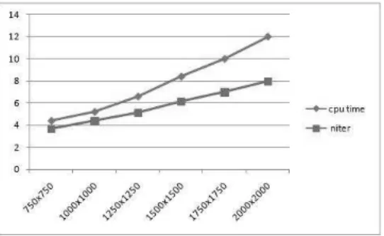
To test the practical effectiveness of our implementations we performed a computational study using randomly generated sparse linear problems. We consider large scale instances where the coefficient matrix A will be large and sparse. It must be mentioned that, sparse linear problems arise in a plethora of applications. We compared the revised Primal Simplex Algorithm (rPSA) with the Primal-Dual Exterior Point Simplex Algorithm (PDEPSA), and the last one with LIPSOL built-in function of MATLAB’s optimization toolbox. This is a variant of Mehrotra’s predictor corrector Interior Point Method (IPM). The algorithms have been coded in MATLAB. Matlab is an interactive environment that provides high performance computational routines. All the test problems were generated with the following properties. All technological constraints are tangent to a unit ball. None of the constraints is redundant. The computing environment had an Intel Core 2 Duo 1,73 GHz and 1 GB DDR2 RAM. The operating system was MS Windows Vista Business 64-bit edition. The reported CPU times were measured in seconds with MATLAB’s built-in function cputime. The figures shown below, are normalized graphs of the results on the ratio of total cpu-time needed and also of the total number of active iterations covered by each algorithm. We used 10 instances at each problem size category starting from 750 to 2,000 with step size equal to 250. The density varies from 5 to 20%.
Figure 2: 10% Density, ratios of rPSA over PDEPSA
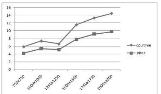
Figure 3: 15% Density, ratios of rPSA over PDEPSA
IPM /PDEPSA
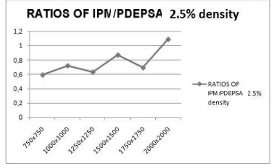
Figure 5: 2.5% Density, ratios of LIPSOL over PDEPSA
IPM /PDEPSA
Figure 6: 5% Density, ratios of LIPSOL over PDEPSA
IPM /PDEPSA
RATIOS OF IPM/PDEPSA
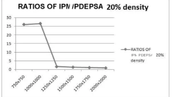
Figure 8: 20% Density, ratios of LIPSOL over PDEPSA
From the figures it is clear that the PDEPSA is far more superior compared to the rPSA for the range of the optimal randomly generated sparse problems. More specifically, the PDEPSA was found to be better in all of our measurements versus Simplex being in the worst case 4,39 times better in terms of cpu - time and 3,66 times better in terms of number of iterations at the size of 750x750, of 2.5% density, and in the best case 14,9 times better in cpu-time and 13,5 times better in number of iterations, at problems of size 2000x2000 and 20% density. This algorithm also showed remarkable stability and robustness versus the IPM algorithm, as densities became larger. That is because for the categories of 10% and 20% density the IPM method failed to solve all problems terminating either saying that the problem is unbounded or infeasible, while PDEPSA did not faced difficulties solving these instances to optimality correctly.
6. CONCLUSION
This paper presents a comparative computational study between the revised primal Simplex algorithm and PDEPSA as well as the built-in IPM algorithm of MATLAB in randomly generated sparse linear problems. All of our computational measurements and the programming of the algorithms were realized into the MATLAB programming environment.
As the results show, PDEPSA is clearly superior to the revised Primal Simplex in all densities and sizes. We should also note here that these differences between these two algorithms would be much larger unless scaling techniques were used for the Simplex algorithm, meanwhile PDEPSA is characterized by the same behavior whether scaling is used or not.
either the problem being unbounded or infeasible. This implies great stability for the PDEPSA which does not fail to solve the problems correctly and in most cases faster than the IPM algorithm.
REFERENCES
[1] Bazaraa, M.S., Jarvis, J.J., and Sherali H.D., Linear Programming and Network Flows, 3rd ed., John Wiley & Sons, 2005.
[2] Bertsimas, D., and Tsitsiklis, J.N., Introduction to Linear Optimization, Athena Scientific, 1997.
[3] Bland, G.R., “New finite pivoting rules for the Simplex method”, Mathematics of Operations
Research, 2 (1977) 103-107.
[4] Dantzig, G.B., Linear Programming and Extensions, Princeton, University Press, Princeton, NJ, 1963.
[5] Erling, D., Andersen, and Yinyu, Ye, “Combining interior-point and pivoting algorithms for Linear Programming”, Management Science, 42 (12) (1996) 1719-1731.
[6] Gondzio, J., “Multiple centrality corrections in a primal-dual method for linear programming”,
Computational Optimization and Applications, 6 (2) (1996) 137-156.
[7] Paparrizos, K., Samaras, N., and Stephanides, G., “A new efficient primal dual simplex algorithm”, Computers and Operations Research, 30 (2003) 1383-1399.
[8] Paparrizos, K., “Pivoting algorithms generating two paths”, presented in ISMP ’97, Lausanne, EPFL Switzerland, 1997.
[9] Samaras, N., “Computational improvements and efficient implementation of two path pivoting algorithms”, PhD Thesis, Department of Applied Informatics, University of Macedonia, 2001. [10] Triantafyllidis, Ch., “Comparative computational study on Exterior Point Algorithms”, BSc