Combined fluvial and pluvial urban flood hazard analysis: method development and application to Can Tho City, Mekong Delta, Vietnam

(1)

NHESSD

3, 4967–5013, 2015

Combined fluvial and pluvial urban flood

hazardanalysis

H. Apel et al.

Title Page

Abstract Introduction

Conclusions References

Tables Figures

◭ ◮

Back Close

Full Screen / Esc

Printer-friendly Version Interactive Discussion

Discussion

P

a

per

|

Discussion

P

a

per

|

Discussion

P

a

per

|

Discussion

P

a

per

|

Nat. Hazards Earth Syst. Sci. Discuss., 3, 4967–5013, 2015 www.nat-hazards-earth-syst-sci-discuss.net/3/4967/2015/ doi:10.5194/nhessd-3-4967-2015

This discussion paper is/has been under review for the journal Natural Hazards and Earth System Sciences (NHESS). Please refer to the corresponding final paper in NHESS if available.

Combined fluvial and pluvial urban flood

hazard analysis: method development

and application to Can Tho City, Mekong

Delta, Vietnam

H. Apel1, O. M. Trepat1, N. N. Hung2, D. T. Chinh1,2, B. Merz1, and N. V. Dung1,2

1

GFZ German Research Centre for Geosciences, Potsdam, Germany

2

Southern Institute of Water Resources Research SIWRR, Ho Chi Minh city, Vietnam

Received: 12 June 2015 – Accepted: 23 July 2015 – Published: 26 August 2015

Correspondence to: H. Apel ([email protected])

(2)

NHESSD

3, 4967–5013, 2015

hazardanalysis

H. Apel et al.

Title Page

Tables Figures

◭ ◮

Back Close

Full Screen / Esc

Discussion

P

a

per

|

Discussion

P

a

per

|

Discussion

P

a

per

|

Discussion

P

a

per

|

Abstract

Many urban areas experience both fluvial and pluvial floods, because locations next to rivers are preferred settlement areas, and the predominantly sealed urban surface prevents infiltration and facilitates surface inundation. The latter problem is enhanced in cities with insufficient or non-existent sewer systems. While there are a number of

5

approaches to analyse either fluvial or pluvial flood hazard, studies of combined flu-vial and pluflu-vial flood hazard are hardly available. Thus this study aims at the analysis of fluvial and pluvial flood hazard individually, but also at developing a method for the analysis of combined pluvial and fluvial flood hazard. This combined fluvial-pluvial flood hazard analysis is performed taking Can Tho city, the largest city in the Vietnamese

10

part of the Mekong Delta, as example. In this tropical environment the annual mon-soon triggered floods of the Mekong River can coincide with heavy local convective precipitation events causing both fluvial and pluvial flooding at the same time. Fluvial flood hazard was estimated with a copula based bivariate extreme value statistic for the gauge Kratie at the upper boundary of the Mekong Delta and a large-scale

hydro-15

dynamic model of the Mekong Delta. This provided the boundaries for 2-dimensional hydrodynamic inundation simulation for Can Tho city. Pluvial hazard was estimated by a peak-over-threshold frequency estimation based on local rain gauge data, and a stochastic rain storm generator. Inundation was simulated by a 2-dimensional hydro-dynamic model implemented on a Graphical Processor Unit (GPU) for time-efficient

20

flood propagation modelling. All hazards – fluvial, pluvial and combined – were ac-companied by an uncertainty estimation considering the natural variability of the flood events. This resulted in probabilistic flood hazard maps showing the maximum inun-dation depths for a selected set of probabilities of occurrence, with maps showing the expectation (median) and the uncertainty by percentile maps. The results are critically

25

(3)

NHESSD

3, 4967–5013, 2015

hazardanalysis

H. Apel et al.

Title Page

Tables Figures

◭ ◮

Back Close

Full Screen / Esc

Discussion

P

a

per

|

Discussion

P

a

per

|

Discussion

P

a

per

|

Discussion

P

a

per

|

1 Introduction

Floods are among the most damaging natural disasters, as statistics of the insurance industry regularly show (MunichRe, 2015). A large share of the damages caused by floods occurs in urban areas, where most of the assets and population are concen-trated. Rapid urban development increases the exposure to floods on the one hand,

5

while climate change including sea level rise increases the hazard, especially in coastal and estuarine regions (Merz et al., 2010). Assessing flood hazard and risk, preparing effective flood mitigation measures and utilizing flood benefits at the same time have thus become an even more vital task in water resources planning and flood manage-ment.

10

In urban areas typically different flood pathways exist. Because locations next to rivers are preferred settlement locations, and because the predominantly sealed urban surface prevents infiltration into the ground both fluvial and pluvial floods typically occur in urban areas. This situation is exacerbated in coastal cities or cities in river deltas, where the low topographical gradient limits the drainage capacity and tidal influences

15

and storm surges can cause additional fluvial inundation. Thus floods of different ori-gins are a main hazard for the world’s river deltas (Renaud et al., 2013; Syvitski and Higgins, 2012; Syvitski, 2008). Particularly prone to this combination of flood types are Asian mega-cities with their extraordinary urban growth, their location at major rivers under a pronounced monsoonal flood regime, and heavy precipitation caused by

cy-20

clones (Chan et al., 2012). Another important aspect particularly in Asia is the low coordination of water resources and flood management of riparian countries in a river basin, where changes in flood hazards can be caused by upstream water management measures, as shown for the Mekong by Kuenzer et al. (2013a).

Despite the large impact of urban inundation by different pathways flood hazard and

25

(4)

NHESSD

3, 4967–5013, 2015

hazardanalysis

H. Apel et al.

Title Page

Tables Figures

◭ ◮

Back Close

Full Screen / Esc

Discussion

P

a

per

|

Discussion

P

a

per

|

Discussion

P

a

per

|

Discussion

P

a

per

|

and risk assessments. Examples for thematic and methodological advances in fluvial hazard or risk assessments are Apel et al. (2004, 2008), Merz and Thieken (2005), Hall et al. (2005), McMillan and Brasington (2008), Vorogushyn et al. (2010), Arrighi et al. (2013), de Bruijn et al. (2014), and Falter et al. (2015).

Pluvial flood hazard analyses are less frequently found in the literature. This can

5

be explained by the inherent complexity of defining and quantifying these events and by the large spatial heterogeneity of the inundation causing rainfall events. Note that this statement refers to hazard analyses, i.e. quantitatively defining rainfall events and their flood impact in a spatially explicit manner including an estimation of the probabil-ity of occurrence of the rainfall events. Traditionally, the probabilprobabil-ity of rainfall events is

10

quantified be Intensity-Duration-Frequency (IDF) curves, which are often established for meteorologically similar regions. But also stochastic, spatially explicit rainfall sim-ulators are used in order to fully describe possible rainfall intensities and their spatial coverage (Burton et al., 2008; Hundecha et al., 2009; Willems, 2001; Wheater et al., 2005). Studies using synthetic rainfall events associated with probabilities of

occur-15

rence for flood inundation modelling for the derivation of pluvial flood hazard maps are, however, not very frequent. Examples for a full pluvial flood hazard analysis are Nuswantoro et al. (2014) or Blanc et al. (2012).

Studies considering the combined effects of fluvial and pluvial flooding are very rare. In fact only two studies were found. Chen et al. (2010) performed a scenario based

20

inundation modelling study considering the combination of fluvial and pluvial floods for a small city area in the UK. A fluvial flood with a return period of 200 years was sim-ulated with a dike overtopping scenario, and a synthetic dike breach scenario. These two fluvial scenarios were combined with rainfall scenarios of different probabilities of occurrence. The rainfall intensity was assumed uniform over the simulation area.

How-25

(5)

NHESSD

3, 4967–5013, 2015

hazardanalysis

H. Apel et al.

Title Page

Tables Figures

◭ ◮

Back Close

Full Screen / Esc

Discussion

P

a

per

|

Discussion

P

a

per

|

Discussion

P

a

per

|

Discussion

P

a

per

|

analysed the joint occurrence of hurricane induced coastal flooding with heavy precipi-tation. But also in this study the probabilities of occurrence of coastal and pluvial floods were not fully defined, as well as the probability of their joint occurrence. Based on these observations this study aims at a joint fluvial and pluvial hazard analysis, where the probabilities of occurrences for both flood types as well as their combinations are

5

quantified. Additionally, spatially explicit probabilistic hazard maps are derived depict-ing the individual as well as the combined hazard. The study also contains an analysis of some natural uncertainty sources, in order to consider the natural variability of the flood triggering events.

The study takes Can Tho city in the Mekong Delta as an example. Can Tho

expe-10

riences both fluvial and pluvial floods, which occur during the monsoon season. Thus both flood types may coincide. A flood hazard or risk analysis has never been per-formed for Can Tho. Flood mitigation planning is, if existing, based on experiences of past floods only. The presented study might therefor be used as a basis for flood mit-igation planning for Can Tho city, if the discussed limitations are taken into account.

15

Can Tho city can be taken as a role model for growing cities in delta regions in the tropics, where fluvial floods and heavy convective rains occur typically in the same pe-riod. Therefore, the developed method might also serve as a blue print for flood hazard analyses in the tropics.

2 Study area and data

20

2.1 Study area

Can Tho city is the largest city and the economic hub in the Vietnamese part of the Mekong Delta with about 1.2 million inhabitants (in 2011). It is located at the junction of the Hau River (Bassac) and the Can Tho River in the Vietnamese part of the Mekong Delta (Fig. 1). The center of the city is the heart of the Ninh Kieu district, located directly

25

(6)

NHESSD

3, 4967–5013, 2015

hazardanalysis

H. Apel et al.

Title Page

Tables Figures

◭ ◮

Back Close

Full Screen / Esc

Discussion

P

a

per

|

Discussion

P

a

per

|

Discussion

P

a

per

|

Discussion

P

a

per

|

to this part of Ninh Kieu, because a Digital Elevation Model (DEM) of sufficient reso-lution was available for this part of the city only. No large scale flood defences exist in Ninh Kieu. However, within the Vietnam Urban Upgrading Project – Can Tho city sub-component (2004–2014) and Mekong Delta Region Urban Upgrading Project – Can Tho city sub-component (2012–2017) road curbs and house entrances were and are

5

elevated in order to reduce inundation of urban areas surrounding major roads. The distance to the coast is about 80 km, but due to the low topography and river gradient the tidal signal is still strong in Can Tho, even during high flood stages. Flood events are thus typically a combination of high water levels during the annual floods combined with a high tide. This results in water levels exceeding the river banks for the

10

time of the semi-diurnal high tides, causing inundations of short duration in the vicinity of the river banks. High water levels in Can Tho causing inundation occur typically late in the flood season during the months September to November (SIWRP, 2010).

Next to the two large rivers a number of channels can be found around and in the city. Inundation can also occur by bank overtopping of these channels. The water levels

15

in these channels at the model domain boundary differ from the main rivers and need to be considered explicitly in a fluvial hazard analysis. However, gauge data for these channels do not exist, and cannot be derived from the gauge in Can Tho. Thus the whole hydraulic system surrounding Can Tho, i.e. the whole Mekong Delta, has to be considered in order to derive consistent boundary conditions for the hydraulic model.

20

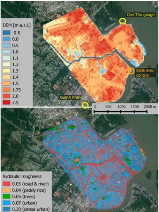
The topography of the city is very low ranging between 1 and 2.5 m a.s.l. (Fig. 2). Most parts of Ninh Kieu are urban areas with built-up houses and infrastructure. Housing typ-ically extends to the very river banks, in cases even exceed them with houses partially on stilts in the rivers or channels.

2.2 Data

25

(7)

NHESSD

3, 4967–5013, 2015

hazardanalysis

H. Apel et al.

Title Page

Tables Figures

◭ ◮

Back Close

Full Screen / Esc

Discussion

P

a

per

|

Discussion

P

a

per

|

Discussion

P

a

per

|

Discussion

P

a

per

|

of open channels and underground pipes. However, the sewer system is reportedly not capable of draining flood waters, neither pluvial nor fluvial, due to its limited capacity. Additionally, the sewer system is not well maintained and malfunctioning in many parts (Huong and Pathirana, 2013) reducing the flood sewer capacity even further. Thus in this study the sewer system is neglected in the hydraulic flood simulations.

5

A land use classification based on high resolution RapdEye satellite data with 5 m resolution was derived by the German Aerospace Centre DLR using the algorithms presented in Huth et al. (2012). The 5 m resolution data was resampled to 15 m to be in line with the DEM. Based on the land use classes 5 roughness classes were derived (Fig. 2). For this study we adopt an urban porosity approach of assigning high

rough-10

ness values to dense built-up areas. This aims at reproducing the hydraulic resistance of buildings to urban inundation flows.

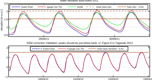
Water level records were collected for the main river gauge of Can Tho in the Hau River and a gauging station installed in the Can Tho River within the WISDOM project (http://www.wisdom.eoc.dlr.de) which was datum-referenced to the main gauge. The

15

locations of the gauges are indicated in Fig. 2 (top panel). A comparison of the recorded and modelled water levels for the flood event 2011 with the bank elevation revealed that the bank elevation as determined by the DEM was too high compared to the gauge records. Even for extraordinary high water levels as experienced during the flood event in 2011 the banks as given in the DEM were not overtopped and thus no inundation

20

would occur (Fig. 3, top panel). This indicates a datum error or at least a discrepancy between gauge data and DEM. Thus the DEM datum had to be corrected. This was performed by comparing the water levels recorded for the flood event in 2011 with the elevation of a river bank stretch along the Hau River (orange circle in Fig. 2, top panel) and information about inundation depths from household surveys near the river (Chinh

25

(8)

NHESSD

3, 4967–5013, 2015

hazardanalysis

H. Apel et al.

Title Page

Tables Figures

◭ ◮

Back Close

Full Screen / Esc

Discussion

P

a

per

|

Discussion

P

a

per

|

Discussion

P

a

per

|

Discussion

P

a

per

|

March 2012. Following their records the bank elevation of the DEM has to be reduced by 0.5 m as well in order to produce a similar picture as in Takagi et al. (2014) compared to the gauge records (Fig. 3, bottom panel). Thus we corrected the datum of the DEM by−0.5 m.

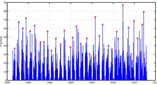
For the pluvial flood hazard analysis hourly rainfall records from the rainfall gauge

5

at Can Tho airport were obtained. These span a time series of 30 years from 1982 to 2012. Figure 4 shows the time series along with the annual maxima. The highest recorded hourly rainfall in this period was 87 mm h−1. The figure shows that the rainfall is distinctively seasonal with high rainfall amounts during the monsoon season (Mai– October) and little rainfall during the remaining time of the year. Next to the annual

10

maximum a large number of additional high rainfall events are obvious in the data series. This calls for a peak over threshold (PoT) approach for the frequency analysis of heavy rainfall events, which will be explained further in Sect. 3.2.

3 Methods

3.1 Fluvial hazard analysis

15

The fluvial hazard analysis comprises two basic components:

1. a 2-D hydraulic model for the simulation of the flood propagation in the study area, and

2. an extreme value statistic for the estimation of the probability of occurrence of flood events of certain magnitudes.

20

(9)

NHESSD

3, 4967–5013, 2015

hazardanalysis

H. Apel et al.

Title Page

Tables Figures

◭ ◮

Back Close

Full Screen / Esc

Discussion

P

a

per

|

Discussion

P

a

per

|

Discussion

P

a

per

|

Discussion

P

a

per

|

3.1.1 Hydraulic model

The hydraulic model for Ninh Kieu was developed on the basis of the 2-dimensional formulation of the shallow water equations solving the momentum (1) and continuity (2) equations numerically as described in Bates et al. (2010):

qt+∆t=

qt−ghflow∆tSf

1+ghflow∆t+n2

|q|

h

10 3 flow

! (1)

5

∂hi,j ∂t =

q_xi−1,j−qi_x,j+q_yi−1,j−qi_y,j

∆xy (2)

where t=time; ∆t=time step; q=specific flow per unit width; i,j=cell indices;

hflow=flow depth between cells;g=acceleration of gravity;n=Manning’s roughness

coe_fficient;Sf=friction slope;h=water depth;∆xy =cell size.

The internal model time step is determined analogously to the Courant–Friedrichs–

10

Levy criterion:

∆tmax=α

∆xy

p

ghflow

(3)

where α denotes an empirical coefficient reducing the time step determined by the Courant–Friedrichs–Levy criterion to ensure model stability.α was set to 0.8.

The implemented model is raster-based and thus able to simulate flood propagation

15

directly on the basis of the provided DEM. Rivers and channels are also modelled in 2-D in contrast to the LISFLOOD-FP implementation of Bates et al. (2010). In order to speed up simulation run-time the code was implemented on a Graphical Processor Unit (NVIDIA Tesla C1060 GPU) using Portland CUDA Fortran. The NVIDIA Tesla C1060 GPU card contains 240 processor cores enabling a highly parallelized execution of the

(10)

NHESSD

3, 4967–5013, 2015

hazardanalysis

H. Apel et al.

Title Page

Tables Figures

◭ ◮

Back Close

Full Screen / Esc

Discussion

P

a

per

|

Discussion

P

a

per

|

Discussion

P

a

per

|

Discussion

P

a

per

|

model code in the spatial domain. The parallelization of the model is handled internally and automatically on a single GPU card and does not require user intervention for domain decomposition and synchronization. This makes the use of GPU for general purpose computing highly attractive. However, code adaptation and reimplementation in CUDA Fortran requires time and effort investment.

5

Hydraulic models need to be calibrated, mainly by adjusting the hydraulic roughness. This was attempted by simulating the large inundation events from 2011. Two large flu-vial events occurred between 26 September and 2 October, and between 24 and 31 October 2011, with peak water levels at 29 September and 29 October, respectively. For these events a household survey was conducted in which the inundation depth

10

was estimated by the house owners (Chinh et al., 2014). Additionally, inundation maps based on TerraSAR-X Stripmap satellite images with 2.75 m spatial resolution covering particular days in the flood season were provided by the German Aerospace Centre DLR. Unfortunately the satellite maps do not cover the peak water levels exactly. For the September event an image one day after the peak water level was available, while

15

for the event in October no image was taken during the entire event. A closer inspection of the flood mask for the 30 September revealed that only little inundation areas are classified within the city limits, in contrast to the actual observed flood. The detected in-undation areas are concentrated on the main roads and wider channels. This behaviour is caused by reflection artefacts of the radar signals from building walls and the close

20

distance of the buildings in streets causing over-radiation of pixels and thus erroneous classification. These intrinsic errors of radar images used for flood mapping in urban areas are reported by Kuenzer et al. (2013b), taking Can Tho city and province as ex-ample. Due to the temporal mismatch and the underestimation of the inundation areas in densely settled areas the flood masks could not be used for the calibration/validation

25

of the hydraulic model, unlike in previous large-scale hydrodynamic modelling studies in the Mekong Delta (Dung et al., 2011; Manh et al., 2014).

(11)

NHESSD

3, 4967–5013, 2015

hazardanalysis

H. Apel et al.

Title Page

Tables Figures

◭ ◮

Back Close

Full Screen / Esc

Discussion

P

a

per

|

Discussion

P

a

per

|

Discussion

P

a

per

|

Discussion

P

a

per

|

floor levels vary greatly in relation to the street level depending on construction de-tails and precautionary measures of the owners, the recorded inundation depths in the house cannot be compared to simulated inundation depths based on the DEM at hand. It was only possible to check the model simulations for plausibility using the informa-tion from the survey as indicators for being inundated or not, i.e. as a rough and not

5

complete estimate for the inundation extent. Figure 5 shows the result of the simulation of the flood 2011 in terms of maximum inundation depths and the reported in-house water depths. The colour code of the simulation and the survey data indicate a plausi-ble model performance in terms of inundation depths, as far as it can be judged from the mismatching inundation data. But it can definitively be stated that at every location

10

of inundated houses the model also simulated an inundation. However, as by far not all flooded households were surveyed, the model performance in terms of overall in-undation extent cannot be assessed conclusively by the data. But given the quality of the DEM and validation data at hand, the performance of the 2-D hydraulic model was assessed as plausible and suitable for the purpose of the study.

15

3.1.2 Boundary conditions of the hydraulic model

In order to simulate meaningful flood propagation boundary conditions have to be pro-vided for the simulation domain along the Hau and Can Tho Rivers as well as for the channels entering the simulation domain on the western border. These boundary con-ditions have to be associated with probabilities of occurrence in order to obtain a hazard

20

analysis. As gauge data su_fficient for an extreme value statistic were not available, par-ticularly for the channels, the boundary conditions for the Can Tho model were derived from a large-scale hydraulic model for the whole Mekong Delta (Dung et al., 2011). The boundary conditions for the Mekong Delta model were derived for the gauge Kratie in Cambodia denoting the upper boundary of the Mekong Delta. A copula-based bivariate

25

extreme value statistic is performed, using annual maximum dischargeQmaxand flood

(12)

NHESSD

3, 4967–5013, 2015

hazardanalysis

H. Apel et al.

Title Page

Tables Figures

◭ ◮

Back Close

Full Screen / Esc

Discussion

P

a

per

|

Discussion

P

a

per

|

Discussion

P

a

per

|

Discussion

P

a

per

|

described in Dung et al. (2015), thus it is not repeated here. From the different statistical models tested in Dung et al. (2015) the Gumbel–Hougaard copula with the marginals of

QmaxandV described by log-normal distributions is used. Synthetic scenarios were

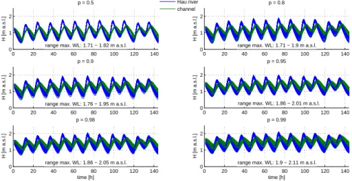
de-rived for probabilities of non-exceedance ofp=0.5, 0.8, 0.9, 0.95, 0.98, 0.99, whereas for each probability level 140 combinations of annual maximum dischargeQmax and

5

flood volumeV were drawn in a Monte-Carlo process from the curves shown in Fig. 7 in Dung et al. (2015). This resulted in altogether 6×140=840 flood scenarios, which were simulated by the large-scale hydraulic model.

From these scenarios the simulated water levels along the Hau River, Can Tho River and the channel were taken as boundary conditions for the 2-D hydraulic model of

10

the study area. To save computational time, the 2-D simulation period was set to 6 days around the maximum water level of each flood scenario at the Hau River. This period is equivalent to the length of the spring tides in the Mekong Delta (Wassmann et al., 2004). This limitation can also be justified from a technical point of view, because sensitivity runs showed that the maximum inundation depth and extent do not change

15

with longer simulation periods. This is due to the distinct tidal influence on the water levels, which exceed the bank levels during maximum water levels, typically during spring tides, and for short periods only. During low tides the water can drain back into the river. Figure 7 shows the Monte Carlo derived boundary conditions for all probability levels for both river and channel.

20

The inundation simulations resulting from these boundary conditions resulted in 140 inundation maps for Can Tho showing maximum inundation depths for every 6 proba-bility levels. For each probaproba-bility level the maximum inundation maps were evaluated per grid cell calculating the median maximum inundation depth and the 5 and 95 % quantiles, as performed by Vorogushyn et al. (2010). These probabilistic hazard maps

25

(13)

NHESSD

3, 4967–5013, 2015

hazardanalysis

H. Apel et al.

Title Page

Tables Figures

◭ ◮

Back Close

Full Screen / Esc

Discussion

P

a

per

|

Discussion

P

a

per

|

Discussion

P

a

per

|

Discussion

P

a

per

|

uncertainty, Merz and Thieken, 2005). Figure 6 summarizes the different steps of the fluvial flood hazard analysis in a flow chart.

3.2 Pluvial hazard analysis

The pluvial hazard analysis comprises three components: a statistical analysis of ex-treme rainfall events in Can Tho, the derivation of spatially distributed synthetic rain

5

storms, and a 2-D hydraulic model. The hydraulic model for the pluvial hazard anal-ysis is the same as described in Sect. 3.1.1, but with different boundary conditions. In order to exclude fluvial inundation the river boundaries were set to low water levels never exceeding the river banks and allowing for outflow from the simulation domain. The boundaries of the model domain were set by adding spatially distributed rainfall

10

volumes derived from the statistical analysis and synthetic rain storms to each grid cell with a time step of 60 s. The statistical analysis and derivation of synthetic rain storms are described in detail in the following sections.

3.2.1 Rainfall extreme value statistics

The basis for this analysis is the 30 year time series of hourly rainfall recorded at Can

15

Tho airport shown in Fig. 4. The presence of many strong rainfall events besides the annual maxima calls for a Peak-over-Threshold (PoT) analysis. PoT enables a full ex-ploitation of the information content of the time series including all hazardous storm events of the monsoon season, and thus a realistic estimation of rainfall probabilities. An inspection of the rainfall time series illustrates the very nature of the rainfall events

20

in the region, which are convective tropical rain storms. Almost all heavy rainfall events have a duration of ≤2 h, with the majority of the events lasting ≤1 h. This suggests that the storm duration for this analysis can be realistically fixed to 1 h. This is also in concordance with local experiences. The construction of Intensity-Duration-Frequency curves is thus not required, a PoT analysis of hourly rainfall is su_fficient to describe the

25

(14)

NHESSD

3, 4967–5013, 2015

hazardanalysis

H. Apel et al.

Title Page

Tables Figures

◭ ◮

Back Close

Full Screen / Esc

Discussion

P

a

per

|

Discussion

P

a

per

|

Discussion

P

a

per

|

Discussion

P

a

per

|

In order to exploit the full information content of the data series, it is assumed that the events lasting two hours in the time series are in fact one hour events extending over the change of the hour. Thus the sums of two hour events are assumed as an event lasting one hour and are used for the PoT analysis. It is assumed that two rainfall events are independent if the temporal distance between them is at least 24 h. In order

5

to determine the optimal threshold for the PoT analysis several tests were conducted: a stability plot of the Generalized Pareto (GP) distribution, which is used for the PoT analysis, a Pareto quantile plot, a mean residual life plot and a Kolmogorov–Smirnov test. In addition, the stability of selected quantiles of the GP was tested depending on different thresholds. The results of the tests are shown in Fig. 8. All the tests

indi-10

cate that a threshold of 18 or 19 mm h−1 is an appropriate choice. Thus the threshold was fixed at 18 mm h−1. Figure 9 shows the resulting maximum likelihood fit of the GP to the PoT series with a threshold of 18 mm h−1 along with the empirical distribution, Gringorten plotting positions of the PoT series, and a fit of a GEV distribution to the annual maxima series for comparison. The PoT quantiles are much higher compared

15

to the annual maximum analysis depicting the likelihood of several extreme rainfall events per year (in the mean 12 rainfall events per year exceeding the threshold of 18 mm h−1). The fitted GP is the basis for the derivation of synthetic storm events and their associated probabilities.

3.2.2 Synthetic storm events

20

In order to simulate inundation caused by heavy rainfalls the statistically derived rainfall intensities recorded at the rain gauge are translated into a spatial rainfall fields, based on the following assumptions:

1. the rainfall events do not cover the whole study area with uniform intensity;

2. the extent of the convective rainfall cell is assumed to be circular;

(15)

NHESSD

3, 4967–5013, 2015

hazardanalysis

H. Apel et al.

Title Page

Tables Figures

◭ ◮

Back Close

Full Screen / Esc

Discussion

P

a

per

|

Discussion

P

a

per

|

Discussion

P

a

per

|

Discussion

P

a

per

|

3. the intensity of the rainfall of the convective cell is highest at its centre and de-creasing to the border;

4. the intensity within the circular extent is distributed according to a Gaussian bell;

5. the intensity along the border of the convective cell is 1/10 of the maximum inten-sity;

5

6. the diameter of the storm cell increases with intensity;

7. the location of the storm cell is stationary during the event duration of 1 h.

Assumption 1 is based on local observations and has been confirmed by regional me-teorologists in personal communication. Assumption 2 is also confirmed by meteo-rologists dealing with radar rainfall observations in the region. A similar assumption

10

was also taken by Nuswantoro et al. (2014) for a storm generator for Jakarta in In-donesia, which has similar rainfall characteristics as the South of Vietnam. Assump-tions 3 to 6 are also based on observaAssump-tions in the area and have also been used by Nuswantoro et al. (2014) for Jakarta. Assumption 4 is reasonable for tropical rain storm cells. This approach of describing the rainfall intensity has been adopted from

15

the weather generator of Willems (2001). For assumption 6 the extent of the large storm events was estimated at approx. 8 km, based on detailed meteorological simu-lations of two large storm events in Can Tho (both around 80 mm h−1) by Huong and Pathirana (2013). Table 1 lists the assumed relation of probability of non-exceedance

p, rainfall intensity R(p), and extent of the storm cells (Full Width at Tenth of

Maxi-20

mum FWTM). The functional relation between FWTM andR(p) was empirically derived as FWTM=R(p)×90, based on the simulated storm events in Huong and Pathirana (2013). Figure 10 shows two synthetic storm events resulting from this procedure for probabilities of non-exceedance of 0.5 and 0.99.

In order to compensate for the negligence of the movement of convective storm cells

25

(16)

NHESSD

3, 4967–5013, 2015

hazardanalysis

H. Apel et al.

Title Page

Tables Figures

◭ ◮

Back Close

Full Screen / Esc

Discussion

P

a

per

|

Discussion

P

a

per

|

Discussion

P

a

per

|

Discussion

P

a

per

|

randomizing the location of the storm centres. Through this procedure the random na-ture of the location of the maximum rainfall is capna-tured, but also the effect of moving rainfall cells can be mimicked. Analogously to the fluvial hazard analysis 140 Monte Carlo runs with random selection of storm centres over the simulation domain for each probability level were conducted. For simulating the inundation caused by the synthetic

5

storm events, the events have to be disaggregated, i.e. the temporal resolution of one hour needs to be reduced to time steps appropriate for the hydraulic model. Instead of a simple uniform disaggregation we opted for a disaggregation with a distinct precipita-tion peak, which is more realistic for heavy convective rains. Thus the hourly intensity of the synthetic storm events was disaggregated into 60 min time steps by a normal

10

distribution withµ=30 min andσ=5 min. This resulted in maximum rainfall intensities at 30 min after precipitation start and a concentration of the bulk of the precipitation in the 30 min surrounding the peak. This temporal disaggregation was applied to every pixel of the synthetic storm events. For the inundation simulation the rainfall amount of the disaggregated storm events was directly added to every pixel covered by the

syn-15

thetic storms as surface water. The surface water was then routed by the 2-D hydraulic model with an overall simulation time of three hours to allow for redistribution of the water after the end of the storm event. The resulting 140 maps of maximum inundation depths per probability level were then evaluated to create probabilistic flood hazard maps. This procedure is identical to the fluvial hazard analysis (cf. Sect. 3.1.2).

20

3.3 Combined hazard analysis

The essential question for a combined fluvial and pluvial hazard analysis is the question of dependency. For this particular study it can be assumed that fluvial and pluvial flood events are completely independent from each other. Although they appear during the same season, which is actually the prerequisite for a joint hazard analysis, the triggers

25

(17)

NHESSD

3, 4967–5013, 2015

hazardanalysis

H. Apel et al.

Title Page

Tables Figures

◭ ◮

Back Close

Full Screen / Esc

Discussion

P

a

per

|

Discussion

P

a

per

|

Discussion

P

a

per

|

Discussion

P

a

per

|

to create urban inundation, but the limited spatial extent and thus rainfall volume does not cause fluvial inundation by the Hau River and channels.

Thus fluvial and pluvial floods can be considered as independent, which has a direct consequence on the calculation of the probabilities of coinciding flood events: in a first step the joint probability of occurrence within a flood season can be quantified by the

5

product of the individual probabilities of occurrences. For example, a joint occurrence of a fluvial flood event with an annual exceedance probability 0.5 and a pluvial flood event of probability 0.5 within the same flood season is 0.25. However, this joint probability of occurrence within the same flood season has to be corrected by the probability that the flood events actually occur at the same time and cause a combined flood event. Thus

10

the probability of occurrence of joint fluvial-pluvial flood events is generally calculated as:

P(fl×pl)=P(fl)×P(pl)×P(co)

withP(co) as the probability of coincidence of fluvial and pluvial flood events.

In this studyP(co) is estimated by the typical length of the flood season and of the

15

fluvial flood events. The period of the flood season in which fluvial inundations in Can Tho typically appear is mid-September to end of November, i.e. lasting about 76 days (cf. Sect. 2.1). Flood peaks of the Mekong with high water levels last typically about 6 days (cf. Sect. 3.1). Within these 6 days 12 distinct flood peaks, i.e. periods of high water levels, occur due to the semi-diurnal tidal regime. The high water levels differ

20

only slightly, as shown in Fig. 7. Furthermore, sensitivity runs with the hydraulic model have shown that the maximum inundation depths of a combined flood event do not differ significantly, if the rain storm event occurs exact at the time of highest water level, or if it occurs within±3 h around high water levels. This means that the sensitive time window for coincidence of a fluvial and pluvial event is 12×6 h=3 days within a flood

25

(18)

NHESSD

3, 4967–5013, 2015

hazardanalysis

H. Apel et al.

Title Page

Tables Figures

◭ ◮

Back Close

Full Screen / Esc

Discussion

P

a

per

|

Discussion

P

a

per

|

Discussion

P

a

per

|

Discussion

P

a

per

|

to account for the uncertainty in the assumption taken for this calculation, a value of

P(co)=0.2 was used for calculating the joint fluvial-pluvial flood probabilities.

A set of joint flood events was simulated by combining fluvial and pluvial flood events with the same individual probability of occurrence. A complete permutation of different probability levels for fluvial and pluvial flood events was not performed in order to obtain

5

the same number of probability levels, but also to keep the required simulation time in manageable limits.

Technically, the combined fluvial and pluvial flood hazard maps were derived by sim-ulating the 140 fluvial flood scenarios per probability level and adding a synthetic rain-storm event with a random rain-storm centre location at the time of the maximum water

10

level of the fluvial scenario boundary. From the 140 combined scenarios per probability level probabilistic hazard maps were derived just as for the fluvial and pluvial analysis. Figure 6 illustrates the combined hazard analysis in the overall process flow chart.

4 Results and discussion

4.1 Fluvial hazard

15

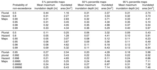
Figure 11 shows the probabilistic fluvial hazard maps comparing the 5, 50, and 95 % percentile maps for all selected probability levels. The inundation maps clearly show the inundation pathways. Inundation of the built-up area starts around the junction of the city channel and the Can Tho River, at the 90◦bend of the city channel in the East of the simulation domain, along the open sewer channel connected to the Can Tho

20

River, and low lying areas around the city channel after the 90◦ bend of the channel in the East of the simulation domain. From these locations the inundation is progressing into the urban area. A particular distinct feature is the inundation of the30 Tháng 4

road (Road of the 30 April) crossing the sewer channel. This is in accordance with

observations during inundation events.

(19)

NHESSD

3, 4967–5013, 2015

hazardanalysis

H. Apel et al.

Title Page

Tables Figures

◭ ◮

Back Close

Full Screen / Esc

Discussion

P

a

per

|

Discussion

P

a

per

|

Discussion

P

a

per

|

Discussion

P

a

per

|

The area most susceptible to inundation is the part of the Cái Kh ´ê ward between the Hau River and the wide part of the city channel. This area is always inundated except for the 5 % quantile map ofplevel 0.5. This is also the area of the deepest inundation. Figure 11 shows that the maximum inundation depths and extents are increasing with increasing probability of non-exceedance, as expected. In the median quantile

5

maps the mean maximum inundation depth excluding the channel and boundary cells evaluates to 0.31 m for the p level of 0.5, and increases to 0.36 m for p level 0.99 (cf. Table 2). This rather slight increase in mean inundation depth is accompanied by a substantial increase in the inundated area from 2.37 km2 (p=0.5) to 5.29 km2(p= 0.99). In the 50 % quantile maps almost all the city area is inundated forplevel 0.99.

10

A further noteworthy feature of Fig. 11 is the di_fference between the quantile maps. There are considerable differences in inundation extent, and for the higher p levels also in inundation depth. This uncertainty is caused by the different pairs of maximum discharge and volume of the synthetic flood events stemming from the extreme value analysis of the fluvial boundary described in Sect. 3.1.2. In the particular context of Can

15

Tho city with prevailing short term flood events, the maximum discharge of the synthetic events and thus the maximum water levels play the dominant role. The maximum water level controls the overbank water level and inundation duration, because with higher maximum water levels also the period of overbank water levels during a tidal cycle of six hours is longer. Contrary to the maximum water level the overall volume of the

20

whole flood season does not have any impact on the local inundation in Can Tho city. Thus the range of the maximum flood discharges determined by the 140 random MC derived boundaries perp level causes the uncertainty in the flood hazard in Can Tho city as shown in Fig. 11.

This uncertainty is also shown in Table 2 comparing the inundated areas between the

25

(20)

NHESSD

3, 4967–5013, 2015

hazardanalysis

H. Apel et al.

Title Page

Tables Figures

◭ ◮

Back Close

Full Screen / Esc

Discussion

P

a

per

|

Discussion

P

a

per

|

Discussion

P

a

per

|

Discussion

P

a

per

|

0.5 shows even higher mean maximum inundation depths as the higher quantile maps. This is a statistical effect caused by the relatively few inundated grid cells, which are along the main inundation hot spots, all of them showing comparatively high maximum inundation depths.

4.2 Pluvial hazard

5

The pluvial hazard maps are shown in the same format as for the fluvial hazard maps in Fig. 12. On first glance the distinctively different characteristics of the pluvial hazard maps become obvious. The hazard maps neither show featured flow paths nor partic-ular hot spots of inundation. This is caused by the nature of the boundary conditions providing spatially distributed input, in combination with the Monte Carlo selection of

10

random storm centre locations. As a result the pluvial hazard maps look much more uniform compared to the fluvial hazard maps. The inundation patterns show the to-pographical depressions as given by the DEM rather than actual flow paths. It has to be mentioned that the proposed methodology of random storm locations and variable spatial extent and intensity of the synthetic rain storms yields characteristically different

15

hazard maps compared to the assumption of spatially uniform coverage of the whole simulation domain. Spatially uniform rain storms would produce different quantile maps, which would look more uniform over the whole simulation domain. And even more im-portant, the inundation depths would be deeper due to the higher rainfall volume given by a uniform coverage compared to the synthetic storm events derived in Sect. 3.2.2.

20

As shown in Table 2 and visible in Fig. 12, the mean maximum inundation depths of the pluvial maps are much lower for allp levels compared to the fluvial hazard maps. For the 50 % quantile maps they range between 6 and 11 cm. However, the inundation extent is higher compared to the fluvial maps due to the spatially distributed rain storms. For the 50 % quantile maps the inundation area is always roughly 1 km2larger.

25

(21)

NHESSD

3, 4967–5013, 2015

hazardanalysis

H. Apel et al.

Title Page

Tables Figures

◭ ◮

Back Close

Full Screen / Esc

Discussion

P

a

per

|

Discussion

P

a

per

|

Discussion

P

a

per

|

Discussion

P

a

per

|

between the quantile maps in terms of inundation extent is much larger with the pluvial hazard maps, particularly for the lower p levels. The uncertainty range given by the quantile maps is actually in the same range as between the median of the lowest and highest p level. This holds true for both mean maximum inundation depths and inundation extent, as shown in Table 2. Solely the mean maximum inundation depth

5

between the quantile maps for p level 0.5 does not follow this rule, because of the same statistical effect in calculating the mean maximum inundation depth for the 5 % quantile map. The wide uncertainty range becomes particularly obvious by comparing the 95 % quantile map for p level 0.5 and the 5 % quantile map for p level 0.99, for both mean maximum inundation depths and inundation extent. These maps are almost

10

identical.

This phenomenon is a direct consequence of the random nature of the location of the storm centres. In the absence of defined inundation pathways, this random distribution of the storm centres causes the di_fferent inundation patterns and thus the character-istics of the quantile maps. The 95 % quantile map of theplevel 0.5 basically shows

15

inundations caused by the centre of a small rain storm hitting by chance a defined are of the simulation domain. On the contrary, the 5 % quantile map of the p level 0.99 show the inundation caused by the borders of a large storm that actually hit another part of the city. Due to the different storm magnitudes this results in similar quantile maps for di_fferent p levels. Assuming that the assumptions for the derivation of the

20

synthetic storm events (cf. Sect. 3.2.2) are reasonable, this is not only a consequence of the proposed method, but also of the very nature of the rain storms causing inunda-tion, and thus a characteristic feature of pluvial hazard maps under a pre-dominantly convective rainfall regime.

4.3 Combined fluvial-pluvial hazard

25

(22)

NHESSD

3, 4967–5013, 2015

hazardanalysis

H. Apel et al.

Title Page

Tables Figures

◭ ◮

Back Close

Full Screen / Esc

Discussion

P

a

per

|

Discussion

P

a

per

|

Discussion

P

a

per

|

Discussion

P

a

per

|

the spatially more uniform but lower inundation depths of the pluvial hazard maps. In general the fluvial inundation is dominant, i.e. causes the deeper inundations, while the pluvial inundation plays a role only in places where no fluvial inundation occurs. These areas are mainly the yet unnamed industrial park in the An Hòa ward at the North-West corner of the simulation domain, and the Thôùi Bình ward west of the 90◦ bend of the

5

domain boundary.

Interestingly, the maximum inundation depths in the fluvial dominated areas differ only slightly (max. a few mm) from the fluvial hazard maps. This indicates that the fluvial processes are not significantly altered by the additional pluvial input. This is caused by the smaller duration and thus flood water volume of the rain storms compared to the

10

fluvial inundation.

The interplay of fluvial and pluvial inundation results in overall larger inundation ex-tents compared to both fluvial and pluvial hazard maps alone (cf. Table 2). The mean maximum inundation depths, however, are lower compared to the fluvial maps, which is again a statistical effect accounting for the larger number of inundated cells with low

15

inundation depths stemming from the pluvial input.

The percentile maps quantifying the natural uncertainty also show features of both fluvial and pluvial uncertainty maps. In the fluvial dominated inundation areas uncer-tainty within each probability level is smaller than the difference between the median of all probability levels. The uncertainty within theplevels is skewed, i.e. the di_fference in

20

inundation extent between the 5 and 50 % percentile maps is larger than between the 50 and 95 % percentile maps. However, for the pluvial dominated inundation areas the same large uncertainty as for the pluvial hazard maps can be observed.

Sensitivity of coincidence

The core assumption of the combined hazard analysis is the exact coincidence of

25

(23)

NHESSD

3, 4967–5013, 2015

hazardanalysis

H. Apel et al.

Title Page

Tables Figures

◭ ◮

Back Close

Full Screen / Esc

Discussion

P

a

per

|

Discussion

P

a

per

|

Discussion

P

a

per

|

Discussion

P

a

per

|

water level was performed. A comparison of the final probabilistic hazard maps with the exact match maps showed only minor differences in maximum inundation depth and extent in the range of a few millimetres. Given the nature of the processes and the uncertainties in the DEM and input data this is negligible. This means that in the combined hazard analysis the specific point in time of coincidence of rain storm and

5

fluvial inundation is not of major importance, at least for the used criteria of maximum inundation depth and extent. It can be suspected that the timing of the rain storm within the fluvial event plays a more pronounced role if fluvial and pluvial events of different probabilities of occurrence are combined, e.g. a fluvial event with p=0.5 combined with a pluvial event of p=0.99. However, as these combinations were not simulated

10

this can be only speculated with the current results at hand.

Spatial coincidence of the flood triggers also proved to be of minor importance. The fact that the maximum inundation depths of the combined analysis do not differ much from the fluvial analysis could indicate that with the given set of 140 Monte Carlo com-binations the random storm centres do not fall in the areas where the fluvial inundation

15

is highest. An increase of the Monte Carlo runs could clarify this question. However, although the simulation time with the models and hardware at hand are in acceptable limits, simulation time is still a prohibitive factor in this respect.

4.4 Implications for risk assessment

Combining fluvial and pluvial flood events in a hazard analysis has implications for

es-20

timating flood risk. In flood risk assessments (FRA), the occurrence of fluvial, pluvial and combined flood events and their probabilities have to be taken into account. While a combination of fluvial and pluvial hazard without any interaction can be considered straightforwardly as the sum of the individual hazards and associated risks, the inclu-sion of the combined hazard requires the consideration that parts of the fluvial and

25

(24)

NHESSD

3, 4967–5013, 2015

hazardanalysis

H. Apel et al.

Title Page

Tables Figures

◭ ◮

Back Close

Full Screen / Esc

Discussion

P

a

per

|

Discussion

P

a

per

|

Discussion

P

a

per

|

Discussion

P

a

per

|

and the damage it inflicts. For a discrete set of scenarios, i.e. probability levels as used in this study, EAD is formulated as:

EAD₌ n X

i=1

∆Pi×Di

with∆P =increment of probability of exceedance= ∆(1−p) withp=probability of non-exceedance,D=damage inflicted,i as the numerator of the probability levels

consid-5

ered, and nas the number of probability levels. As this formulation is an approxima-tion of the integraapproxima-tion of a (hypothetical) continuous risk curve, the probability of ex-ceedance and the damage have to be interpolated between theplevels (Ward et al., 2011; Merz et al., 2009). Using a linear interpolation∆P_i andD_i are defined as:

D_i =1

2(Di+1+Di)

10

∆P_i =P_i₊1−Pi.

If the fluvial (fl) and pluvial (pl) hazard were not coinciding, the EAD for combined fluvial and pluvial risk would be simply the sum of EAD(fl) and EAD(pl). However, in the presented study fluvial and pluvial hazard can coincide, and this has to be taken into account in the calculation of the overall EAD. Formally this is achieved by reducing the

15

probability of exceedance of the individual hazards by the probability of exceedance of the combined hazard:

EAD(fl, pl, fl×pl)= n X

i=1

∆[P(fl)_i−P(fl×pl)_i]×D(fl)_i+ n X

i=1

∆[P(pl)_i−P(fl×pl)_i]×D(pl)_i

+ n X

i=1

∆P(fl×pl)_i×D(fl×pl)_i.

This formulation is valid for the presented combination of fluvial and pluvial

probabil-20

(25)

NHESSD

3, 4967–5013, 2015

hazardanalysis

H. Apel et al.

Title Page

Tables Figures

◭ ◮

Back Close

Full Screen / Esc

Discussion

P

a

per

|

Discussion

P

a

per

|

Discussion

P

a

per

|

Discussion

P

a

per

|

probability levels is performed, the additional scenarios and their probabilities must also be considered analogously as in the special case presented here. Formally this is expressed as an extension of the formula above:

EAD(fl, pl, fl×pl)₌ n X

i=1

∆



P(fl)_i− n X

j=1

P(fl×pl)_i_,_j



×D(fl)_i

+ n X

i=1

∆



P(pl)_i− n X

j=1

P(fl×pl)_i,j 

×D(pl)_i

5

+ n X

i=1 n X

j=1

∆P(fl×pl)_i_,_j×D(fl×pl)_i_,_j.

4.5 Limitations of the approach

Although the presented results appear to be plausible and are accompanied by un-certainty estimations, it is clear that such comprehensive approaches have their limita-tions. This section identifies and discusses the most important limitalimita-tions.

10

The developed methodology considers the natural (aleatory) uncertainty only, i.e. the uncertainty stemming from the natural variability of the flood triggering events. In the fluvial analysis the variability of the occurrence of flood peak and flood volume, and the hydrograph shape at the upper boundary of the Mekong Delta was taken into account in this respect. In the pluvial analysis natural variability was mapped by the magnitude

15

and location of rain storm events. However, the quantification of these uncertainties is also plagued with uncertainty, which is termed epistemic uncertainty. This generally stems from imperfect knowledge of the processes, insufficient data or models. For example, for the fluvial analysis Dung et al. (2015) showed that the bivariate frequency analysis is associated with considerable epistemic uncertainty stemming from a limited

20

(26)

NHESSD

3, 4967–5013, 2015

hazardanalysis

H. Apel et al.

Title Page

Tables Figures

◭ ◮

Back Close

Full Screen / Esc

Discussion

P

a

per

|

Discussion

P

a

per

|

Discussion

P

a

per

|

Discussion

P

a

per

|

Technically, a consideration of this uncertainty source would mean an extension of the Monte Carlo analysis, in which even more pairs of flood peakQmaxand flood volumeV

per probability level have to be considered. Whether this is feasible, is mainly a question of simulation time. The resulting percentile maps would certainly show a wider range as compared to this study. The same holds true if other epistemic uncertainty sources

5

were considered.

Also the pluvial analysis contains epistemic uncertainty which was also not quanti-fied. The epistemic uncertainty is associated to the assumptions listed in Sect. 3.2.2. Particularly the assumptions on storm extent and spatial distribution of intensity have large impacts on the inundation simulation and thus the probabilistic hazard maps.

Un-10

fortunately, no data for the validation of the assumptions was available to the authors, and thus a quantification of the uncertainty caused by the assumptions cannot be per-formed. An evaluation of radar rain images of the area would be of great benefit in this respect.

Further sources of epistemic uncertainty are the hydraulic model and the quality of

15

the DEM. While the horizontal resolution is acceptable for a study of this scale, the quality of the vertical information has to be critically assessed. Because the DEM was interpolated from elevation information of topographical maps, it has to be expected that the accuracy is actually not sufficient for urban inundation simulation. Additional uncertainty is caused by the lack of calibration and validation of the hydraulic model

20

due to insufficient data. However, sensitivity runs with different distributions and values of roughness parameters indicate that the uncertainty in maximum inundation depths is dominated by the topography and not by the parameterization of roughness values.

These uncertainties have to be taken into account when using the derived hazard maps for actual flood management planning. It is recommended to use the maps mainly

25

(27)

NHESSD

3, 4967–5013, 2015

hazardanalysis

H. Apel et al.

Title Page

Tables Figures

◭ ◮

Back Close

Full Screen / Esc

Discussion

P

a

per

|

Discussion

P

a

per

|

Discussion

P

a

per

|

Discussion

P

a

per

|

5 Conclusions

This study develops a methodology for a combined fluvial and pluvial flood hazard analysis. The methodology is exemplarily developed for Can Tho city, which is the economic centre of the Vietnamese part of the Mekong Delta. Both fluvial and pluvial inundation processes cause regular flooding in Can Tho city. Both fluvial and pluvial

5

hazard analyses contain a dedicated statistical part to estimate the probabilities of occurrence of floods of different magnitudes. Synthetic flood events were derived based on this frequency analysis, which provide the boundary conditions for a 2-dimensional inundation modelling of the central part of the city. With the help of the hydraulic model maximum inundation depths were determined for every flood scenario for Can Tho city.

10

The two flood hazards were not only considered independent from each other, but also in combination, i.e. occurring at the same time. Because fluvial and pluvial flood-ing occurs in the same period of the year, these events can coincide. As the triggerflood-ing events are essentially independent from each other, the probability of occurrence of coinciding events can be directly calculated from the probability of occurrences of the

15

individual events and the probability of coincidence of the events. The resulting in-undation events bear features of both fluvial and pluvial inin-undation processes. The presented method is novel not only in terms of the specific application for Can Tho city, but also in general, as a similar study has not been published so far. The presented methods can be transferred to other cities in a similar tropical setting, and adapted to

20

different climate zones.

The hazard analyses also include uncertainty estimations. For fluvial, pluvial, and combined hazards the natural uncertainty, i.e. variability of flood events with identi-cal probabilities of occurrence, was taken into account. This facilitated the derivation of probabilistic hazard maps showing the maximum inundation depths with an

expec-25

(28)

NHESSD

3, 4967–5013, 2015

hazardanalysis

H. Apel et al.

Title Page

Tables Figures

◭ ◮

Back Close

Full Screen / Esc

Discussion

P

a

per

|

Discussion

P

a

per

|

Discussion

P

a

per

|

Discussion

P

a

per

|

management and mitigation plans, for a flood risk assessment for Can Tho city, or for cost-benefit analyses of flood protection measures.

However, for usage of the hazard maps in practical applications the limitations, resp. the epistemic uncertainty, which was not quantified, have to be taken into account. In this respect the quality of the digital elevation model and the assumptions underlying

5

the derivation of synthetic rain storm events have the highest impact on the final haz-ard estimates, particularly the maximum inundation depths. Thus for the time being, the maps should be mainly used for the determination of the most affected areas, and the maximum inundation depths should be taken as rough guidance only. Considering the prominent damage pathways – inundation of houses by water levels in the streets

10

exceeding road curbs – a possible way of direct usage of the maps could be to target flood mitigation plans to areas with maximum inundation depths exceeding a certain threshold, e.g. 10 cm. This would eliminate the random character of the pluvial maps and thus the influence of the assumptions taken on rain storm extent and storm centre locations. In order to increase the overall confidence in the hazard maps, the

assump-15

tions on rains storms should be validated, preferably by an analysis of a series of rain radar maps. Additionally, an improved DEM should be obtained and the hydraulic sim-ulations repeated.

In any case, the presence of two or more hazard sources and their combination have to be taken into account in any risk assessment in a statistically sound and consistent

20

manner. In general, the probability of occurrence of combined flood events reduces the probabilities of occurrence of individual fluvial and pluvial events of the same magni-tude, which needs to be reflected in the risk calculations. How this can be achieved, has been exemplarily shown for a hypothetical calculation of Expected Annual Damage EAD, a standard risk variable.

25