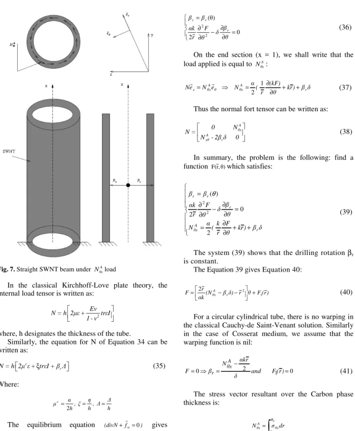
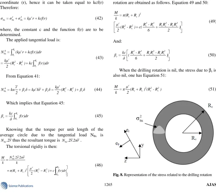
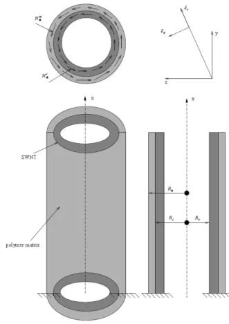
A COSSERAT-TYPE PLATE THEORY AND ITS APPLICATION TO CARBON NANOTUBE MICROSTRUCTURE

This research concerns about the development and application of a mathematical model, based on the Saint-Venant hydrodynamic equations, to study the behavior of the propagation of a

The probability of attending school four our group of interest in this region increased by 6.5 percentage points after the expansion of the Bolsa Família program in 2007 and

Comparison of numerical results of the pressure coefficient upstream and downstream of the second baffle plate with experimental results measured at the channel wall. Comparison

This log must identify the roles of any sub-investigator and the person(s) who will be delegated other study- related tasks; such as CRF/EDC entry. Any changes to

Além disso, o Facebook também disponibiliza várias ferramentas exclusivas como a criação de eventos, de publici- dade, fornece aos seus utilizadores milhares de jogos que podem

Durante o estágio percebi que nos dias de hoje, a notoriedade e importância dos medicamentos não só a nível clínico como também económico, reitera a valorização da

Afinal, se o marido, por qualquer circunstância, não puder assum ir a direção da Família, a lei reconhece à mulher aptidão para ficar com os poderes de chefia, substituição que

É nesta mudança, abruptamente solicitada e muitas das vezes legislada, que nos vão impondo, neste contexto de sociedades sem emprego; a ordem para a flexibilização como