An artificial neural network model for rainfall forecasting in Bangkok, Thailand

(1)

HESSD

5, 183–218, 2008

A rainfall forecast model using Artificial

Neural Network

N. Q. Hung et al.

Title Page

Abstract Introduction

Conclusions References

Tables Figures

◭ ◮

Back Close

Full Screen / Esc

Printer-friendly Version

Interactive Discussion

Hydrol. Earth Syst. Sci. Discuss., 5, 183–218, 2008 www.hydrol-earth-syst-sci-discuss.net/5/183/2008/ © Author(s) 2008. This work is distributed under the Creative Commons Attribution 3.0 License.

Hydrology and Earth System Sciences Discussions

Papers published inHydrology and Earth System Sciences Discussionsare under open-access review for the journalHydrology and Earth System Sciences

An artificial neural network model for

rainfall forecasting in Bangkok, Thailand

N. Q. Hung, M. S. Babel, S. Weesakul, and N. K. Tripathi

School of Engineering and Technology, Asian Institute of Technology, Thailand

Received: 14 December 2007 – Accepted: 17 December 2007 – Published: 30 January 2008 Correspondence to: N. Q. Hung (nguyenquang.hung@ait.ac.th)

(2)

HESSD

5, 183–218, 2008

Neural Network

N. Q. Hung et al.

Title Page

Tables Figures

◭ ◮

Back Close

Full Screen / Esc

Interactive Discussion Abstract

The present study developed an artificial neural network (ANN) model to overcome the difficulties in training the ANN models with continuous data consisting of rainy and non-rainy days. Among the six models analyzed the ANN model which used general-ized feedforward type network and a hyperbolic tangent function and a combination of

5

meteorological parameters (relative humidity, air pressure, wet bulb temperature and cloudiness), and the rainfall at the point of forecasting and rainfall at the surrounding stations, as an input for training of the model was found most satisfactory in forecasting rainfall in Bangkok, Thailand. The developed ANN model was applied to derive rainfall forecast from 1 to 6 h ahead at 75 rain gauge stations in the study area as forecast point

10

from the data of 3 consecutive years (1997–1999). Results were highly satisfactory for rainfall forecast 1 to 3 h ahead. Sensitivity analysis indicated that the most important input parameter beside rainfall itself is the wet bulb temperature in forecasting rainfall. Based on these results, it is recommended that the developed ANN model can be used for real-time rainfall forecasting and flood management in Bangkok, Thailand.

15

1 Introduction

Accurate information about rainfall is essential for the use and management of water resources. In the urban areas, rainfall has a strong influence on traffic control, the oper-ation of sewer systems, and other human activities. Nevertheless, rainfall is one of the most complex and di_fficult elements of the hydrology cycle to understand and to model

20

due to the tremendous range of variation over a wide range of scales both in space and time (French et al., 1992). The complexity of the atmospheric processes that gen-erate rainfall makes quantitative forecasting of rainfall an extremely di_fficult task. Thus, accurate rainfall forecasting is one of the greatest challenges in operational hydrology, despite many advances in weather forecasting in recent decades (Gwangseob and

25

(3)

HESSD

5, 183–218, 2008

Neural Network

N. Q. Hung et al.

Title Page

Tables Figures

◭ ◮

Back Close

Full Screen / Esc

The development of Artificial Neural Networks (ANN), which perform nonlinear map-ping between inputs and outputs, has lately provided alternative approaches to fore-cast rainfall. ANN were first developed in the 1940s (Mc Culloch and Pitts, 1943), and the development has experienced a renaissance with Hopfield’s effort (Hopfield, 1982) in iterative auto-associable neural networks. In recent decades, the developed

algo-5

rithms have helped overcome a number of limitations in the early networks, making the practical applications of ANN more applausible. Based on the structure of the neural networks and the learning algorithm, various neural network models have been studied and targeted at solving di_fferent sets of problems.

Neural networks have been widely applied to model many of nonlinear hydrologic

10

processes such as rainfall-runo_ff (Hsu et al., 1995; Shamseldin, 1997), stream flow (Zealand et al., 1999; Campolo and Soldati, 1999; Abrahart and See, 2000), ground-water management (Rogers and Dowla, 1994), ground-water quality simulation (Maier and Dandy, 1996; Maier and Dandy, 1999), and rainfall forecasting. More detailed discus-sion regarding the application of ANN in hydrology can be referred to in the special

15

technical report of Journal of Hydrologic Engineering (ASCE, 2000). A pioneer work in applying ANN for rainfall forecasting was undertaken by French et al. (1992), which em-ployed a neural network to forecast two-dimensional rainfall, 1 hour in advance. Their ANN model used only present rainfall data, generated by a mathematical rainfall simu-lation model, as input for training data set. This work is, however, limited in a number

20

of aspects. For example, there is a trade-o_ffbetween the interaction and the training time, which could not be easily balanced. The numbers of hidden layers and hidden nodes seem insufficient, in comparison with the numbers of input and output nodes, to reserve the higher order relationship needed for adequately abstracting the process. Still, it has been considered as the first contribution to ANN’s application and

estab-25

lished a new trend in understanding and evaluating the roles of ANN in investigating complex geophysical processes.

(4)

HESSD

5, 183–218, 2008

Neural Network

N. Q. Hung et al.

Title Page

Tables Figures

◭ ◮

Back Close

Full Screen / Esc

the rainfall time series. In the study, monthly rainfall was used as input data for train-ing model. The authors analyzed 87 years of rainfall data in Kerala, a state in the southern part of the Indian Peninsula. The empirical results showed that neuro-fuzzy systems were efficient in terms of having better performance time and lower error rates compared to the pure neural network approach. In some cases, the deviation of the

5

predicted rainfall from the actual rainfall was due to a delay in the actual commence-ment of monsoon, El-Ni ˜no Southern Oscillation (ENSO).

Another study of ANN that relates to El-Ni ˜no Southern Oscillation was done by Manusthiparom et al. (2003). The authors investigated the correlations between El Ni ˜no Southern Oscillation indices, namely, Southern Oscillation Index (SOI), and sea

10

surface temperature (SST), with monthly rainfall in Chiang Mai, Thailand, and found that the correlations were significant. For that reason, SOI, SST and historical rain-fall were used as input data for standard back-propagation algorithm ANN to forecast rainfall one year ahead. The study suggested that it might be better to adopt various related climatic variables such as wind speed, cloudiness, surface temperature and air

15

pressure as the additional predictors.

Toth et al. (2000) compared short-time rainfall prediction models for real-time flood forecasting. Di_fferent structures of auto-regressive moving average (ARMA) models, artificial neural networks and nearest-neighbors approaches were applied for forecast-ing storm rainfall occurrforecast-ing in the Sieve River basin, Italy, in the period 1992–1996 with

20

lead times varying from 1 to 6 h. The ANN adaptive calibration application proved to be stable for lead times longer than 3 h, but inadequate for reproducing low rainfall.

Another application was described by Koizumi (1999), who employed an ANN model using radar, satellite and weather-station data together with numerical products gen-erated by the Japan Meteorological Agency (JMA) Asian Spectral Model for 1-year

25

(5)

HESSD

5, 183–218, 2008

Neural Network

N. Q. Hung et al.

Title Page

Tables Figures

◭ ◮

Back Close

Full Screen / Esc

more training data became available. It is still unclear to what extent each predictor contributed to the forecast and to what extent recent observations might improve the forecast.

In summary, results from past studies have shown that ANN is a good approach to forecast rainfall. The ANN model is capable to model without prescribing

hydrologi-5

cal process, catching the complex nonlinear relation of input and output, and solving without the use of differential equations (Luk et al., 2000; Hsu et al., 1995; French et al., 1992). In addition, ANN could learn and generalize from examples to produce meaningful solution even when the input data contain errors or incomplete (Luk et al., 2000). In fact, while the numbers of studies on application of ANN in rainfall forecasting

10

using discontinuous time series data are conducted, studies on continuous time series data are few. Most of the studies in the past used discrete data to train ANN model, training data was screen out from collected (and/or generated) data so it contains only rainy time (i.e., rainfall events or monthly rainfall data). Because the models are trained with rainy input data, and are typically ran in batch mode, the output forecast is issued

15

only after the occurrence of the rainfall events. It means that these models can predict rainfall only when rain occurs, they can tell how long the rain will last but not whether it will rain or not. When using continuous past rainfall data which contained both rain and no rain days as input to train ANN model, no rain periods with zero value makes no change in weights update process so ANN could not recognize the pattern and give

20

low accuracy result. For those reasons, most of the study of ANN on rainfall forecast in the past is not suitable to apply in real time forecasting.

The main objective of this paper is to develop real time ANN based rainfall forecasting model using observed rainfall records in both space and time. In order to overcome the problem encountered in training ANN model with continuous data, an optimum

25

(6)

HESSD

5, 183–218, 2008

Neural Network

N. Q. Hung et al.

Title Page

Tables Figures

◭ ◮

Back Close

Full Screen / Esc

for 3 yr (1997 to 1999). Moreover, aside from the rainfall data, additional predictors such as relative humidity, air pressure, wet bulb temperature, cloudiness, and rainfall from surrounding rain gauge stations, were also adopted to improve the prediction accuracy. Sensitivity analysis is also taken in account to grade the important factor of each input to the model performance.

5

2 Study area

Bangkok, the capital and also the largest city in Thailand, is also one of the highly de-veloped cities of Southeast Asia. Having a land area of 1569 km2, it is located in the central part of the Thailand on the low, flat plain of the Chao Phraya River, with latitude 13.45◦_{N and longitude 100.35}◦_{E. The city which sits at a distance extending from 27}

10

to 56 km from the river mouth adjacent to the Gulf of Thailand, has a tropical type of climate with long hours of sunshine, high temperatures and high humidity. There are three main seasons; Rainy (April–October), Winter (November–January) and Summer (February–March). The average low temperature is approximately in low to mid 20◦_C

and high temperature in mid 32◦_{C (Thai Meteorological Department, 2005). Bangkok}

15

receives a very high average annual rainfall of 1500 mm and is influenced by the sea-sonal monsoon. The city is a_ffected by flood in a regular basis. When rainfall comes, most of the daily activities are nearly paralyzed. Some of the immediate consequences of a heavy rainfall in Bangkok are: water clogging in the streets, heavy traffic jams, blackouts, and direct or indirect economic losses.

20

The flood events in Bangkok occur from two sources: the rainfall and the rise in water level in Chao Phraya River due to large flow from upstream. In the past, most of the occurrence of high river flow and heavy rains in the city resulted in severe flooding. However, with the construction of a dam upstream and a dike along the riverbank in Bangkok, nearly all parts of the city are now protected from flooding. Land use in

25

(7)

HESSD

5, 183–218, 2008

Neural Network

N. Q. Hung et al.

Title Page

Tables Figures

◭ ◮

Back Close

Full Screen / Esc

The construction of drainage infrastructure has not kept pace with land-use change due to lack of funds. Hence, capacity of the drainage system has become more and more insu_fficient. In addition, lack of hydrological information and the failure of gravity to effectively remove drainage water from the city make urban flooding inevitable during the wet season. For a developing city like Bangkok, one of the best ways to cope

5

with the flooding problem is to provide advance rainfall forecasting and flood warning. Knowing the condition of rainfall in Bangkok in advance can help in managing and dealing with problems due to flooding.

The Department of Drainage and Sewage (DDS) of Bangkok Metropolitan Admin-istration (BMA) had established Bangkok Metropolitan Flood Control Center (FCC) in

10

1990 for systematic and e_fficient management of operation and control of flood pro-tection facilities. BMA has 53 online tipping bucket type rain gauge stations scattered throughout Bangkok and sensors installed at the canal gates and pumping stations that collect water level data. The observed data is transferred in real time to FCC by UHF radio signals every 15 min. Furthermore, Thai Meteorological Department (TMD) owns

15

a network of 51 rain gauge stations covering Bangkok and nearby areas. Both rain gauge networks consist of rain gauges of tipping bucket type with 0.5 mm accuracy. These data are now available in the Internet and can be used for online applications. Locations of these rain gauges are shown in Fig. 1.

At present, there is no reliable rainfall forecast mechanism using rain gauge data.

20

Bangkok uses only radar data with the SCOUT program to forecast rainfall (Chum-chean et al., 2005). Based upon the historical data (rain gauge data) and the current situation, the flood forecast analysis is manually carried out at FFC. After a decision about control policy is made based on this analysis, the flood control protection com-mand is then broadcasted to all remote control stations (gates and pumping station).

25

(8)

HESSD

5, 183–218, 2008

Neural Network

N. Q. Hung et al.

Title Page

Tables Figures

◭ ◮

Back Close

Full Screen / Esc

tolerance and adoptability, has been selected to be a tool for short-term rainfall fore-cast for Bangkok area. The model is mimic design, so it can be applied not only to Bangkok area but also to other tropical developing urban areas as well.

Historical rainfall data was collected from 104 stations of BMA and TMD rain gauge networks in order to train ANN model. After analysis and screening of data, only 75

5

stations inside Bangkok area were used to train ANN model, while the other 29 stations which are located outside Bangkok were discarded. Meteorological data collected from TMD contains hourly measurement of seven parameters: cloudiness, relative humidity, wet bulb temperature, dry bulb temperature, air pressure, wind speed and average hourly rainfall intensity of all rain gauges.

10

Figure 2 shows the average monthly rainfall in Bangkok for a period from 1991 to 2003. It is observed that there are two peaks of rainfall during one year, the first in May, and the second in October. Climatological data during the period 1991–2004 showed that the average annual relative humidity was about 81% with the average maximum relative humidity of 93% and average minimum relative humidity of 52%. The data also

15

showed that the average annual temperature was 26.8◦_{C, with average maximum}

tem-perature of 33.4◦_{C in April and average minimum temperature of 20.4}◦_{C in December.}

Rainfall data revealed an annual rainfall of 1869.5 mm with the highest average monthly rainfall of approximately 381 mm observed in October, and the lowest average monthly rainfall of about 12 mm occurring in December, usually the driest month of the year.

20

3 Artificial Neural Network

An artificial neural network is an interconnected group of artificial neurons that has a natural property for storing experiential knowledge and making it available for use. The artificial neuron uses a mathematical or computational model for processing of infor-mation based on a connectionist approach to computation, akin to a human brain. In

25

(9)

HESSD

5, 183–218, 2008

Neural Network

N. Q. Hung et al.

Title Page

Tables Figures

◭ ◮

Back Close

Full Screen / Esc

to biological systems, involving adjustments to the synaptic connections that exist be-tween the neurons. Learning often occurs by example through training or exposure to a trusted set of input/output data where the training algorithm iteratively adjusts the connection weights (synapses), and these connection weights store the knowledge necessary to solve specific problems.

5

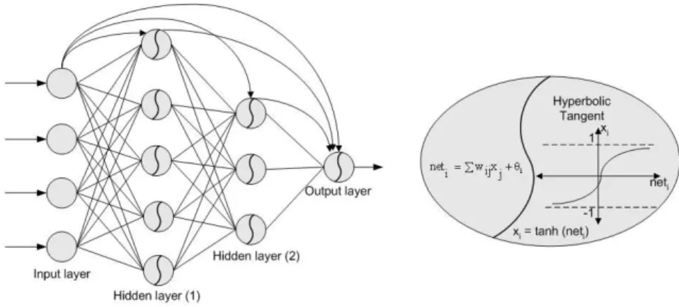
The multilayer perceptron (MLP) is one of the most widely implemented neural net-work topologies. Generally speaking, for static pattern classification, the MLP with two hidden layers is a universal pattern classifier. MLPs are normally trained with the back-propagation algorithm. In fact the renewed interest in ANN was in part triggered by the existence of back-propagation. The back-propagation rule propagates the errors

10

through the network and allows adaptation of the hidden units. Two important char-acteristics of the multilayer perceptron are: its nonlinear processing elements (PEs) which have a nonlinearity that must be smooth (the logistic function and the hyperbolic tangent are the most widely used); and their massive interconnectivity (i.e. any element of a given layer feeds all the elements of the next layer).

15

The multilayer perceptron is trained with error-correction learning, which means that the desired response for the system must be known. Error correction learning works in the following way: from the system response at PE_i at iterationn, di(n), and the desired

responseyi(n) for a given input pattern, an instantaneous errorei(n) is defined by

ei(n)=di(n)−yi(n) (1)

20

Using the theory of gradient-descent learning, each weight in the network can be adapted by correcting the present value of the weight with a term that is proportional to the present input and error at the weight, i.e.

w_{i j}(n+1)=w_{i j}(n)+ηδ_i(n)x_j(n) (2)

The local errorδi(n) can be directly computed from ei(n) at the output PE or can be 25

(10)

HESSD

5, 183–218, 2008

Neural Network

N. Q. Hung et al.

Title Page

Tables Figures

◭ ◮

Back Close

Full Screen / Esc

learning is an improvement to the straight gradient descent in the sense that a memory term (the past increment to the weight) is used to speed up and stabilize convergence. In momentum learning the equation to update the weights becomes

wi j(n+1)=wi j(n)+ηδi(n)xj(n)+α(wi j(n)−wj(n−1)) (3)

where α is the momentum. Normally α should be set between 0.1 and 0.9. The

5

standard back-propagation algorithm is as follow:

1. Initialize all weights and bias (normally a small random value) and normalize the training data.

2. Compute the output of neurons in the hidden layer and in the output layer using

neti = X

wi jxi+θi; xi =transferfunction(neti) (4)

10

1. Compute the error and weight update.

2. Update all weights, bias and repeat steps 2 and 3 for all training data.

3. Repeat steps 2 to 4 until the error has reached to an acceptable level.

Generalized feedforward networks are a generalization of the MLP such that connec-tions can jump over one or more layers. In theory, a MLP can solve any problem that

15

a generalized feedforward network can solve. In practice, however, generalized feed-forward networks often solve the problem much more efficiently. A classic example of this is the two-spiral problem. Without describing the problem, it su_ffices to say that a standard MLP requires hundreds of times more training epochs than the generalized feedforward network containing the same number of processing elements. A simple

20

(11)

HESSD

5, 183–218, 2008

Neural Network

N. Q. Hung et al.

Title Page

Tables Figures

◭ ◮

Back Close

Full Screen / Esc

of a training algorithm. There are two important issues concerning the implementation of artificial neural networks, that is, specifying the network size (the number of layers in the network and the number of nodes in each layer) and finding the optimal values for the connection weights.

In the process of specifying the network size, an insu_fficient number of hidden nodes

5

causes di_fficulties in learning data whereas an excessive number of hidden nodes might lead to unnecessary training time with marginal improvement in training out-come as well as make the estimation for a suitable set of interconnection weights more di_fficult (Zealand et al., 1999). There is no specific rule to determine the appropriate number of hidden nodes; yet the common method used is trial and error based on a

10

total error criterion. This method starts with a small number of nodes, gradually in-creasing the network size until the desired accuracy is achieved. Fletcher and Goss (1993) proposed a suggestion number of node in the hidden layer ranging from (2n+1) to (2√n₊m) wherenis the number of input node, andmis the number of output node. The number of input and output nodes is problem-dependent, and the number of input

15

nodes depends on data availability. In addition, the selection of input should be based on priori knowledge of the problem, prevailing synoptic weather condition over study area. A firm understanding of the hydrologic system under consideration is necessary for the effective selection of input data (Ahmad and Simonovic, 2005).

Regarding the second issue, several training processes are available to find the

val-20

ues of connection weights. These algorithms di_ffer in how the weights are obtained. The selection of training algorithm is related to the network type, computer memory, and the input data. As implied in this study, the standard back propagation algorithm is used in ANN training based on its most popular success, but still there are others, such as QuickProp (QP), Orthogonal Least Square (OLS), Levemberg-Marquart (LM),

25

(12)

HESSD

5, 183–218, 2008

Neural Network

N. Q. Hung et al.

Title Page

Tables Figures

◭ ◮

Back Close

Full Screen / Esc

step in the direction of the negative gradient of the error function during each iteration. The advantage of this algorithm lies in its simplicity.

4 ANN models

In this study, ANN model was applied for each of 75 rain gauge stations in Bangkok, to forecast rainfall from 1 to 6 h ahead as forecast point. Six distinctive alternative models

5

were initially tested in one station in order to find the optimum ANN model which can then be employed for all others stations. Station E18, located in the Sukhumvit area, where a real-time flood forecasting system is currently developed, was chosen as a sample station in order to design the ANN model structure. To enable the selection of the best model, the training data set should include the high, medium and low rainfall

10

periods. Therefore, 1997, 1998 and 1999 rainfall data were chosen as the training data sets, and the 1998 data was chosen as the cross-validation data set. Detailed description of the six models are presented in Table 1.

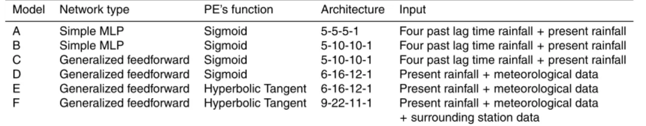
The first model (A) used multilayer perceptron network with simple structure, five nodes in the input layer, two hidden layer with 5 hidden nodes in each of the two layers,

15

and one node in the output layer corresponding to the observed hourly rainfall. Inputs to the model were present hourly rainfall data (t) and four hour lag time of E18 station from (t−4) to (t−1), while the output was rainfall intensity of the next hour (t+1). The transfer function in nodes is the well-known sigmoid function. For the second model (model B), the network type, transfer function and input of training data set were kept

20

unchanged but the number of hidden nodes in both hidden layers were increased from 5 to 10.

In the third model (C), network type was changed from simple MLP to Generalized feedforward network. Data used to train the model was the same as the previous two models (A and B). The fourth model (D) adopted Generalized feedforward,

net-25

(13)

exten-HESSD

5, 183–218, 2008

Neural Network

N. Q. Hung et al.

Title Page

Tables Figures

◭ ◮

Back Close

Full Screen / Esc

sive prior knowledge of all processes involved. However, a good understanding of the physics involved, and a hypothesis on how di_fferent processes (and their state variable) interact with each other would help in evaluating the generality of the relationship when analyzing data. Therefore, the data sets used for training should represent the phys-ically based dynamic range of the forecast. Triggered by this idea, five meteorology

5

parameters were added into the training data set, but the past rainfall data was not included since the data brings more zero value to the training process (for no rain pe-riod). This resulted to six input data for model D, which included relative humidity, wet bulb temperature, air pressure, cloudiness, average hourly rainfall intensity of all rain gauges, and present rainfall of E18 station. Hence the model structure was modified

10

by changing input nodes to 6, increasing the number of node in the first hidden layer to 16, changing the second hidden layer to 12, but still 1 node in the output layer.

The fifth model (E) retains the same model structure as model D, except the transfer function, where the tanh function was used instead of the sigmoid function. In the last model (F), the rainfall data of stations around E18 were considered. A correlation

anal-15

ysis was applied to 75 rain gauge stations in Bangkok to determine which stations are strongly related to E18. Results of the analysis revealed higher correlation of stations E00, E19 and E26 with E18 compared with other stations. Thus the present hourly rainfall data of these three stations were added to the training data set of model E for the formulation of model F. The change in input data resulted to an increase in the

20

number of node in input layer to 9, increase in the number of hidden nodes to 22 and 11 for the first and second hidden layers, respectively.

5 Results and discussion

5.1 Comparison of ANN model

The one hour forecast accuracy of all six ANN models was evaluated by calculating

25

(14)

HESSD

5, 183–218, 2008

Neural Network

N. Q. Hung et al.

Title Page

Tables Figures

◭ ◮

Back Close

Full Screen / Esc

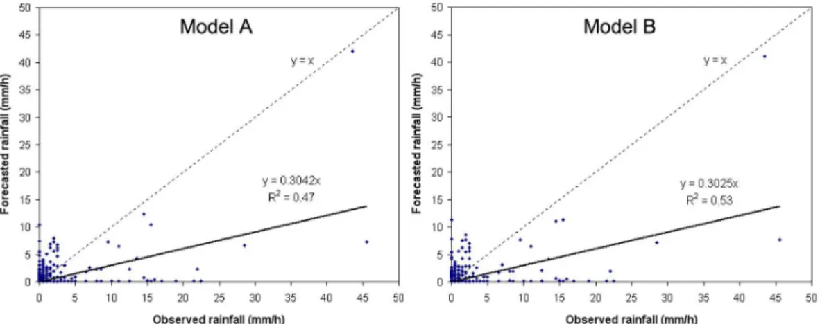
Error (RMSE) and Correlation Coe_fficient (R2), described in Table 2. From the training results of ANN models, forecasted rainfall was plotted against the observed data to determine the relationship of these two variables (Figs. 5, 7 and 9). It was observed that the RMSE for all models seemed to be small at less than 2 mm per hour. This value however, does not seem to be significant since the total number of rainy period

5

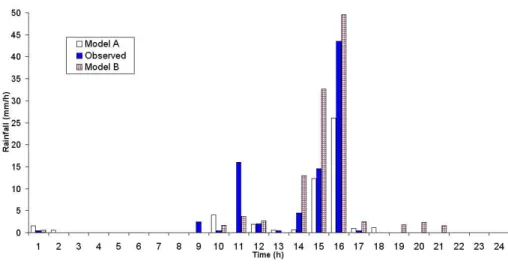
in both forecasted and observed data are very small compared to the total patterns of training data. Example of 24 h computation on 21 August 1998 for each model were also plotted (Figs. 4, 6 and 8) for a better view of the difference between forecasted value and observed data.

Model A gave very low accuracy forecast with EI of only 27.32% and 29.08% for

10

training stage and testing stage, respectively, and correlation coefficient of 0.47 in the training stage and 0.41 in the testing stage. The less number of nodes (only 5) in each of the two hidden layers in this model may not be su_fficient to memorize and learn the problem. Moreover, the computation time for a fixed 100 000 iteration was around 36 h. This model could not reach to the stopping criteria and result fluctuated with longer

15

time of training. Model B with more number of hidden nodes gave a slightly better result, with EI reaching 37.25% and 36.5% in the training stage and the testing stage, respectively andR2of 0.53 in the training stage and 0.51 in testing stage. This model also has a better RMSE value at 1.72 mm/h compared with model A (1.88 mm/hour). The computation time for training with 100 000 iterations was around 24 h. A sample of

20

24 h computation on 21 August 1998 of models A and B plotted against the observed data is shown in Fig. 4. Both models gave some false forecast and the forecasted rainfall differed with observed data from few to more than 20 mm/h. It was observed in the scatter plot in Fig. 5 that the linear trend line of models A and B are under the 1:1 line, indicating that the forecast from these two models are underestimated.

25

(15)

general-HESSD

5, 183–218, 2008

Neural Network

N. Q. Hung et al.

Title Page

Tables Figures

◭ ◮

Back Close

Full Screen / Esc

ized feedforward network worked better than simple multilayer perceptron network. For Model D, the change of input of training data improved the results with higher EI val-ues of 50.17% and 49.5% in the training stage and testing stage, respectively. For both models C and D, RMSE value is less than 2 mm/h, indicating minimal change compared with RMSE of models A and B, but viewed in the Fig. 6, the gap between

5

forecasted rainfall of model C and D and observed data is much more smaller than that of models A and B (Fig. 4). As shown in Fig. 7 where the trend line in the scatter graph is still laid down under the 1:1 line, with the small angle presenting a low correlation coe_fficient value (0.56 for model C and 0.64 for model D), indicating these two models still gave overestimation of rainfall forecast. On the contrary, the addition of

meteo-10

rology parameters such as relative humidity, air pressure above mean sea level, total cloudiness, wetbulb temperature, and average rainfall of all stations, into the training data set for model D improved the accuracy of forecast.

For model E, the use of hyperbolic tanh function instead of the sigmoid function brought a very interesting result. The EI of the model levels up to 66.71% and 68.5%

15

in the training stage and in the testing stage, respectively, withR2 of 0.69 in training stage and 0.71 in testing stage. As seen in Figure 8, forecasting for the same day of 21 August, 1998 using model E, resulted to better accuracy. The tanh function with the range of each neuron in the layer between−1 and 1 showed a better performance compared with the sigmoid function where the range of each neuron in the layers is

20

between 0 and 1.

Model F gave the highest performance in terms of efficiency and forecasting. The efficiency attained at 1 h is between 97.35% and 96.52% in the training stage and testing stage, respectively. A scatter plot of model F (see Fig. 9) shows that the trend line almost coincided with the 1:1 line, corresponding to a correlation coefficient of 0.96.

25

(16)

HESSD

5, 183–218, 2008

Neural Network

N. Q. Hung et al.

Title Page

Tables Figures

◭ ◮

Back Close

Full Screen / Esc

5.2 Sensitivity analysis

While training a network, the effect that each of the network inputs is having on the network output should be studied. This provides feedback as to which input channels are the most significant, based on which we may decide to prune the input space by removing the insignificant parameters. This will reduce the size of the network, which

5

in turn reduces the complexity and the training time. Sensitivity analysis is a method for extracting the cause and e_ffect relationship between the inputs and outputs of the network. This work is done by removing each input channel in turn and then comparing the statistical indicator such as EI, RMSE andR2.. The greater the effect observed in the output, the greater the sensitivity with respect to the input. In order to ensure

10

the accurate output from the model, the input sensitive analysis was carried out and compared with the results from model F. As mentioned in the preceding section, the inputs into the final model (F) are total cloudiness, air pressure (HPa), relative humidity (%), wetbulb temperature ( ˚ C), average rainfall from TMD (mm/h), rainfall from three surrounding stations (strongly connected with station E18) (mm/h), and rainfall from

15

E18 station (mm/h), 6 alternative models were run for the sensitivity analysis. These 6 alternative models maintained the same network architecture, using the tanh function and forecasting rainfall 1 h ahead.

As can be seen from Table 3, the most significant input is wetbulb temperature. The model running without wetbulb temperature as input obtained an EI reduced from

20

97.35% of that of the model F, to 80.62% in the training stage. The second most important parameter is humidity since in the model without humidity, EI was down to 83.22% in the training stage. Other important parameters are pressure and rainfall from surrounding station. The average rainfall of all stations collected from the main TMD station RS26 stays as the fifth important parameter, with an EI decreasing to 86.37% for

25

(17)

HESSD

5, 183–218, 2008

Neural Network

N. Q. Hung et al.

Title Page

Tables Figures

◭ ◮

Back Close

Full Screen / Esc

5.3 Rainfall forecasting

Based on the results of designing stage with six models tested on station E18, model F which gave the highest performance in term of efficiency and forecasting was em-ployed to forecast rainfall from 1 to 6 h ahead for all 75 stations. Three years rain-fall and meteorology data were available, so model performance was evaluated using

5

cross-validation to maximize data available for training. By this method, performance statistics can be generated for the entire 3 y period. To evaluate the performance of models, the same three indices EI, RMSE andR2 were used. Table 4 expresses the summarized ANN results of maximum, minimum, mean EI,R2, and RMSE for rainfall forecasting from 1 to 6 h ahead of all stations. There is a consistency in the

perfor-10

mance of models, where ANN model is quite stable and gave almost the same result for all stations. It also shows that the model performance decreases with the increasing lead time forecast. Average EI of 1 and 2 h forecast is 0.86 and 0.69, respectively. How ever, these values continue to decrease to 0.54 for 3 h forecast, 0.45 for 4 h forecast, 0.41 for 5 h forecast and finally drops to 0.36 in the 6 h forecast. Correlation coefficient

15

and RMSE show the same trend where meanR2 decreases from 0.88 for 1 h forecast to 0.6 at 6 h forecast, and RMSE value increases from 0.87 mm/hr to 1.93 mm/h from 1 h to 6 h forecast, respectively. From Table 4, it can be seen that ANN models provide remarkable accuracy predictions for 1 and 2 h. For 1 h forecast, some stations can get EI up to outstanding value of 0.98, while the lowest EI value of all stations is 0.74.

Cor-20

relation coefficient also presents a notable maximum value of 0.99 and minimum value 0.74. For 2 h forecast, results is also quite good where maximum EI is 0.87, minimum EI is 0.63; andR2 is in the range from 0.92 to 0.63. Forecasting results of 3 hours is not so good but still there are some stations which could come up with EI of up to 0.68 andR2gained value of 0.84. Forecasting for 4 to 6 h ahead gave poor results, event

25

maximumR2 value varies in the range from 0.78 to 0.71, but the range of EI is only from 0.62 to 0.48.

(18)

HESSD

5, 183–218, 2008

Neural Network

N. Q. Hung et al.

Title Page

Tables Figures

◭ ◮

Back Close

Full Screen / Esc

example, with station E18, total rainfall pattern for the year 1998 is 312, and total training pattern for this period is 5928. Thus, in term of mm/h, the RMSE value is always very small, but it is not mean that forecast result is well fit with observed data, So, to check whether the peak forecast is fit or not, it also need visual checking. Example of comparison between observed rainfall (left figure) and predicted rainfall (right figure)

5

for 1 to 6 h ahead forecasting at 8 August 1998, is shown in Fig. 10. In this figure, co-ordinates of all stations, the observed rainfall data and the predicted rainfall data for all 75 stations are fed into the Surfer program for plotting the rain map. Therefore, the comparison of the observed and forecasted rainfall for the whole Bangkok area can be seen clearly. The Kriging method was used for scattered data interpolation. As

10

seen in Fig. 10, at 8 h, there were light rain at some stations and 1 h forecast could forecast quite accurately. At 9 h, rain became heavier on the east side of Bangkok, forecasting of 2 h also presented a nice shape of rain map, but there were some stations giving false forecast, and darker legend color also indicates underestimated prediction. Rainfall forecast at 3 h ahead also gave underestimated result in most stations. The

15

rain moved into the center of the area (observed at 10 h), but in the 3 h forecast, rain not only appeared in the center but also in left lower corner of the map. From 11:00 h to 13:00 h, rain has reduced and stopped, but in the forecast result, there were still rainfall at some stations. Figure‘10 revealed a similar conclusion as Table 4, that is, rainfall forecast for 3 to 6 h is not so good, but is still considered to be a reasonable non-linear

20

approximation. By presenting forecast result in rain map, this could provide a better view of the whole picture of rainfall forecast for all stations in the area.

6 Conclusions

In this study, an Artificial Neural Network model has been developed to run real time rainfall forecast for Bangkok, Thailand, with lead time from 1 to 6 h. Rain gauge data

25

(19)

mod-HESSD

5, 183–218, 2008

Neural Network

N. Q. Hung et al.

Title Page

Tables Figures

◭ ◮

Back Close

Full Screen / Esc

els were tested to identify the appropriate model design to overcome the difficulty of training ANN with continuous rainfall data. Comparison of 1 h rainfall forecast of these six models showed that combination of meteorology data with rainfall data as training data has significantly improved the forecast accuracy. Result of designing stage also concluded that Generalized Feedforward network and hyperbolic tanh function proved

5

to work well in this study. With appropriate network architecture, ANN model is able to learn from continuous data which contained both rain and no rain period, thus the model can be adopted to run online forecasting.

While ANN is considered as data driven approaches, and the selecting of input data in this study was limited on the availability of the data, it is still important to determine

10

the dominant model inputs, as this increases the generalization ability of the network for a given data. Furthermore, it can help reducing the size of the network and conse-quently reduces the training times. Choosing suitable parameters for the ANN models is more or less a trial and error approach. In this study, sensitive analyses were used in conjunction with judgment to rank the important factor of each input to the model

15

performance.

The ANN model in this study is very robust, characterized by fast computation, ca-pable of handling the noisy and approximate data that are typical in weather data. The predicted values of all 75 stations matched well with the observed rainfall in case of forecasts with short lead times, 1 or 2 h. Not only that, the rainfall forecasting for 3 h

20

ahead using ANN also provided reasonable results. The e_fficiency indices were grad-ually reduced as the forecast lead time increased from 4 to 6 h. Although the model performance of 6 h forecasting was low and the forecasting was not as accurate as expected, this model still has some practical applications in flood management for the study area. Overall, the study indicates that the use of time series analysis techniques

25

(20)

HESSD

5, 183–218, 2008

Neural Network

N. Q. Hung et al.

Title Page

Tables Figures

◭ ◮

Back Close

Full Screen / Esc

area.

Acknowledgements. This article is a part of doctoral research conducted by the first author at Water Engineering and Management, Asian Institute of Technology, Bangkok, Thailand. The financial support provided by the DANIDA for pursuing the study is gratefully acknowledged. The author would like to express sincere gratitude to the staffof Thai Meteorological

Depart-5

ment and Bangkok Metropolitan Administration for providing, sourcing and facilitating access to and usage of invaluable data and information used in this study. Thanks are also extended to the anonymous reviewer and the editor for their constructive contributions to the manuscript.

References

Abraham, A., Steinberg, D., and Philip, S. N.: Rainfall forecasting using soft computing

mod-10

els and multivariate adaptive regression splines, available at:http://meghnad.iucaa.ernet.in/ ∼nspp/ieee.pdf)2001.

Abrahart, R. J. and See, L.: Comparing neural network and autoregressive moving average techniques for the provision of continuous river flow forecast in two contrasting catchments, Hydrol. Process., 14, 2157–2172, 2000.

15

Ahmad, S. and Simonovic, S. P.: An artificial neural network model for generating hydrograph from hydro-meteorological parameters, J. Hydrol., 315(1–4), 236–251, 2005.

ASCE: Task committee on Application of Artificial Neural Networks in Hydrology, Part I, J. Hydrol. Eng., 5(2), 115–123, 2000.

ASCE: Task committee on Application of Artificial Neural Networks in Hydrology, Part 2, J.

20

Hydrol. Eng., 5(2), 124–137, 2000

Campolo, M. and Soldati, A.: Forecasting river flow rate during low-flow periods using neural networks, Water Resour. Res., 35 (11), 3547–3552, 1999.

Chumchean, S., Einfalt, T., Vibulsirikul, P., and Mark, O.: To prevent floods in Bangkok: An operational radar and RTC application – Rainfall forecasting, 10th International Conference

25

on Urban Drainage, Copenhagen, Denmark, 21–26 August 2005.

Coulibaly, P., Anctil, F., and Bobee, B.: Daily reservoir inflow forecasting using artificial neural networks with stopped training approach, J. Hydrol., 230, 244–257, 2000.

Fletcher, D. S. and Goss, E.: Forecasting with neural network: An application using bankruptcy data, Inform. Manage., 24, 159–167, 1993.

(21)

HESSD

5, 183–218, 2008

Neural Network

N. Q. Hung et al.

Title Page

Tables Figures

◭ ◮

Back Close

Full Screen / Esc

French, M. N., Krajewski, W. F., and Cuykendall, R. R.: Rainfall forecasting in space and time using neural network, J. Hydrol., 137, 1–31, 1992.

Gwangseob, K. and Ana, P.B.: Quantitative flood forecasting using multisensor data and neural networks, J. Hydrol., 246, 45–62, 2001.

Hopfield, J. J.: Neural networks and physical systems with emergent collective computational

5

abilities, Proc. Natl. Acad. Sci., 79, 2554–2558, 1982.

Hsu, K., Gupta, H. V., and Sorooshian, S.: Artificial neural network modeling of the rainfall-runoffprocess, Water Resour. Res., 31(10), 2517–2530, 1995.

Koizumi, K.: An objective method to modify numerical model forecasts with newly given weather data using an artificial neural network, Weather Forecast., 14, 109–118, 1999.

10

Luk, K. C., Ball, J. E., and Sharma, A.: A study of optimal model lag and spatial inputs to artificial neural network for rainfall forecasting, J. Hydrol., 227, 56–65, 2000.

Maier, R. H. and Dandy, G. C.: The use of artificial neural network for the prediction of water quality parameters, Water Resour. Res., 32 (4), 1013–1022, 1996.

Maier, R. H. and Dandy, G.C.: Comparison of various methods for training feed-forward neural

15

network for salinity forecasting, Water Resour. Res., 35 (8), 2591–2596, 1999.

Manusthiparom C., Oki T., and Kanae, S.: Quantitative Rainfall Prediction in Thailand, First In-ternational Conference on Hydrology and Water Resources on Asia Pacific Region (APHW), Kyoto, Japan, 13–15 March 2003.

Mc Culloch W. S. and Pitts, W.: A logical calculus of the ideas immanent in nervous activity, B.

20

Math. Biophys., 5, 115–133, 1943.

Rogers, L. L. and Dowla, F. U.: Optimization of groundwater remediation using artificial neu-ral networks with paneu-rallel solute transport modeling, Water Resour. Res., 30 (2), 457–481, 1994.

Shamseldin, A. Y.: Applacation of a neural network technique to rainfall-runoff modeling, J.

25

Hydrol., 199, 272–294, 1997.

Toth, E., Montanari, A., and Brath, A.: Comparison of short-term rainfall prediction model for real-time flood forecasting, J. Hydrol., 239, 132–147, 2000.

Zealand, C. M., Burn, D. H., and Simonovic, S. P.: Short term streamflow forecasting using artificial neural networks, J. Hydrol., 214, 32–48, 1999.

(22)

HESSD

5, 183–218, 2008

Neural Network

N. Q. Hung et al.

Title Page

Tables Figures

◭ ◮

Back Close

Full Screen / Esc

Interactive Discussion Table 1.Alternative models considered in the study.

Model Network type PE’s function Architecture Input

A Simple MLP Sigmoid 5-5-5-1 Four past lag time rainfall+present rainfall B Simple MLP Sigmoid 5-10-10-1 Four past lag time rainfall+present rainfall C Generalized feedforward Sigmoid 5-10-10-1 Four past lag time rainfall+present rainfall D Generalized feedforward Sigmoid 6-16-12-1 Present rainfall+meteorological data E Generalized feedforward Hyperbolic Tangent 6-16-12-1 Present rainfall+meteorological data F Generalized feedforward Hyperbolic Tangent 9-22-11-1 Present rainfall+meteorological data

(23)

HESSD

5, 183–218, 2008

Neural Network

N. Q. Hung et al.

Title Page

Tables Figures

◭ ◮

Back Close

Full Screen / Esc

Interactive Discussion Table 2.Performance statistics of ANN models.

Index

A B C D E F

Model Training (1997–1999 data)

EI (%) 27.32 37.25 44.15 50.17 66.71 97.35 RMSE (mm/h) 1.88 1.72 1.87 1.65 1.46 0.89

R2 0.47 0.53 0.56 0.64 0.69 0.96

Testing (1998 data)

EI (%) 29.08 36.57 43.28 49.65 68.57 96.52 RMSE (mm/h) 1.84 1.75 1.78 1.58 1.41 0.88

(24)

HESSD

5, 183–218, 2008

Neural Network

N. Q. Hung et al.

Title Page

Tables Figures

◭ ◮

Back Close

Full Screen / Esc

Interactive Discussion Table 3.Performance statistics for sensitivity analysis.

Model F Without Without Without Without Without Without

Index Cloudiness Relative Humidity Air pressure surrounding station TMD rain Wetbulb temperature

Training (1997–1999 data)

EI (%) 97.35 87.49 83.22 86.47 86.37 89.41 80.62

RMSE (mm/h) 0.89 0.82 0.79 0.81 0.78 0.91 0.78

R2 0.96 0.95 0.91 0.93 0.93 0.95 0.89

Testing (1998 data)

EI (%) 96.52 94.4 92.57 93.54 93.65 95.49 82.57

RMSE (mm/h) 0.88 0.79 0.78 0.82 0.83 0.88 0.75

(25)

HESSD

5, 183–218, 2008

Neural Network

N. Q. Hung et al.

Title Page

Tables Figures

◭ ◮

Back Close

Full Screen / Esc

Interactive Discussion Table 4.Summary of ANN results for rainfall forecasting at 75 rainfall stations.

Lead Efficiency Correlation RMSE

Index Coefficient

(26)

HESSD

5, 183–218, 2008

Neural Network

N. Q. Hung et al.

Title Page

Tables Figures

◭ ◮

Back Close

Full Screen / Esc

(27)

HESSD

5, 183–218, 2008

Neural Network

N. Q. Hung et al.

Title Page

Tables Figures

◭ ◮

Back Close

Full Screen / Esc

(28)

HESSD

5, 183–218, 2008

Neural Network

N. Q. Hung et al.

Title Page

Tables Figures

◭ ◮

Back Close

Full Screen / Esc

(29)

HESSD

5, 183–218, 2008

Neural Network

N. Q. Hung et al.

Title Page

Tables Figures

◭ ◮

Back Close

Full Screen / Esc

(30)

HESSD

5, 183–218, 2008

Neural Network

N. Q. Hung et al.

Title Page

Tables Figures

◭ ◮

Back Close

Full Screen / Esc

(31)

HESSD

5, 183–218, 2008

Neural Network

N. Q. Hung et al.

Title Page

Tables Figures

◭ ◮

Back Close

Full Screen / Esc

(32)

HESSD

5, 183–218, 2008

Neural Network

N. Q. Hung et al.

Title Page

Tables Figures

◭ ◮

Back Close

Full Screen / Esc

(33)

HESSD

5, 183–218, 2008

Neural Network

N. Q. Hung et al.

Title Page

Tables Figures

◭ ◮

Back Close

Full Screen / Esc

(34)

HESSD

5, 183–218, 2008

Neural Network

N. Q. Hung et al.

Title Page

Tables Figures

◭ ◮

Back Close

Full Screen / Esc

(35)

HESSD

5, 183–218, 2008

Neural Network

N. Q. Hung et al.

Title Page

Tables Figures

◭ ◮

Back Close

Full Screen / Esc

Interactive Discussion Fig. 10. Comparison between observed rainfall (left side figures) and predicted rainfall (right

(36)

HESSD

5, 183–218, 2008

Neural Network

N. Q. Hung et al.

Title Page

Tables Figures

◭ ◮

Back Close

Full Screen / Esc