Aplicação da Análise de Séries Temporais
para Detecção e Prognóstico de Danos em
Estruturas Inteligentes
Ilha Solteira
CAMPUS DE ILHA SOLTEIRA
Wagner Francisco Rezende Cano
Aplicação da Análise de Séries Temporais
para Detecção e Prognóstico de Danos em
Estruturas Inteligentes
Dissertação apresentada ao Programa de Pós-Graduação em Engenharia Mecânica, Facul-dade de Engenharia Mecânica de Ilha Solteira – UNESP como parte dos requisitos necessários
para obtenção do título de Mestre em Engen-haria Mecânica.
Área do Conhecimento: Mecânica dos Sóli-dos.
Orientador: Prof. Dr. Samuel da Silva
Cano, Wagner Francisco Rezende.
C227a Aplicação da análise de séries temporais para detecção e prognóstico de danos em estruturas inteligentes / Wagner Franciso Rezende Cano. – Ilha Solteira: [s.n.], 2015
67 f. : il.
Dissertação (mestrado) – Universidade Estadual Paulista. Faculdade de Engenharia de Ilha Solteira. Área de conhecimento: Mecânica dos Sólidos, 2015
Orientador: Samuel da Silva Inclui bibliografia
First of all, I wold like to thank my parents, Solange and Wagner, and family for all the support throughout such special moment of my life. Also, I am thankful for the company and help of my girlfriend Camila.
I am thankful to Professor Samuel da Silva for the opportunity to keep developing my research. I am also thankful to Professor Vicente Lopes Júnior, Professor João Antonio Pereira and Professor Mike Brennan for the advises which were very useful to accomplish this work.
I would like to thank the members of GMSINT and Carlos “Grilo” Santana for always being helpful and to contribute to my academic and personal growth.
I am thankful to the SHM staff of CPqD – Paulo Henrique de Oliveira Lopes, Bernardo José Guilherme de Aragão and Edmilson Sanches Silva – for offering their lab and expertise. I am also pleased for the opportunity to be part of their staff.
I would like to acknowledge the financial support provided by the following Brazil-ian funding agencies: Research Foundation of São Paulo (FAPESP) by grant number 12/09135-3 and National Council for Scientific and Technological Development (CNPq) by grant number 470582/2012-0.
I am also thankful to FAPEMIG and CNPq for partially funding the present research work through the National Institute of Science and Technology in Smart Structures in Engineering (INCT-EIE).
Esse trabalho apresenta uma abordagem baseada no processamento de séries temporais para tratar o problema de detecção e o prognóstico de danos em estruturas com sensores e atuadores piezelétricos acoplados considerando as possíveis variabilidades ambientais e operacionais. A primeira abordagem se baseia na identificação de um modelo autorregres-sivo de predição construído com um sinal temporal de resposta de referência. Métricas indicativas de danos são extraídas dos erros de predição e a separação de efeitos (carrega-mento ou danos) é feita por um algoritmo de agrupa(carrega-mento fuzzy. Esse procedi(carrega-mento é implementado em uma estrutura de material compósito ensaiada em um sistema para teste de materiais de modo a reproduzir condições de carregamento a fim de simular condições reais de operação da estrutura. Por outro lado, a segunda metodologia proposta emprega uma identificação de dois estágios. Primeiramente, um modelo autorregressivo é criado para o monitoramento estrutural como no procedimento anterior, porém, utilizando o controle estatístico de processos para detectar um dano progressivo. Em seguida, modelos autorregressivos com entradas exógenas são estimados para as condições de referência e de dano para acompanhar as variações de parâmetros e permitir a realização de um prognóstico sobre a condição estrutural futura da estrutura. Testes iniciais em uma placa de alumínio mostraram que este método é capaz de realizar um prognóstico razoável e predizer o comportamento dinâmico da estrutura associado com um nível específico de redução de massa. Ambos métodos e resultados são discutidos e comparados ao final do trabalho.
This work presents an approach based on time series processing to deal with the damage detection and prognosis issue in structures coupled with piezoelectric sensors and actuators considering eventual operational and environmental variabilities. The first approach is based on the identification of a predictive autoregressive model obtained with a reference time response. Damage indicative metrics are extracted from prediction errors and the separation of effects (loading or damage) is performed by a fuzzy clustering algorithm. This procedure is carried on a composite structure attached to a material test system to reproduce loading conditions in order to simulate real operational conditions. On the other hand, the second proposed methodology employs a two step identification. First, an autoregressive model is created for structural monitoring similarly to the previous procedure, but employing statistical process control to detect progressive damage. Next, autoregressive models with exogenous inputs are estimated for reference and damaged conditions in order to track variation of parameters, allowing the prognosis of the structure’s future structural condition. Initial tests on an aluminum plate indicated that this method is capable of performing a reasonable prognosis and predicting structure’s dynamic behavior associated to a specific level of mass reduction. Both methods and results are discussed and compared by the end of the work.
A – Norm-inducing matrix
A – Polynomial acting on the output signal a – Coefficient of polynomial A
B – Polynomial acting on the input signal C – Centroid of a cluster
c – Number of clusters
cL – Lamb wave longitudinal mode velocity
cP – Lamb wave phase velocity
cT – Lamb wave transverse mode velocity
e – Discrete prediction error vector (V) f – Discrete frequency vector (Hz) h – Plate thickness
J – Function to be minimized by the fuzzy clustering analysis
j – imaginary number
k – Discrete sample l – Discrete sample
m – Number of elements in a damage index subgroup N – Number of samples or realizations
n – Number of damage index subgroups na – Number of a coefficients
nb – Number of b coefficients
nθ – Number of estimated coefficients
p – Relative position of clusters q – Backshift operator
S – Mean of Si values
Si – Standard deviation of each damage index subgroup
t – Discrete time vector (s)
U – Left singular vector
u – Discrete input signal vector (V)
y – Discrete output signal vector (V)
ˆ
y – Vectory adjusted by an autoregressive model (V)
γ – γ index
¯
γ – Mean γ index ξ – Wavenumber µ – Mean operator
σ – Standard deviation operator
Σ – Diagonal matrix from the single value decomposition Σii – Diagonal terms of matrix Σ
ACF – Autocorrelation function AIC – Akaike’s information criterion AR – Autoregressive model
ARM A – Autoregressive moving average model
ARX – Autoregressive model with exogenous inputs BSS – Baseline signal stretch
CCDM – Correlation coefficient deviation metric CL – Center line
CP qD – Centro de Pesquisa e Desenvolvimento em Telecomunicações
F P E – Final prediction error M T S – Material test system
1 Overview of the effect separation procedure. . . 27
2 Composite structure coupled with two Smart® PZT sensor patches. . . 28
3 Reference signals and dispersion curves for the composite structure. . . 29
4 Response signals under loading effect. . . 29
5 Validation of the reference AR model. . . 31
6 Prediction errors. . . 32
7 Damage indices calculated for the clustering method (❩ – γ index, ◊ – CCDM, Ԃ – trace). . . 33
8 Three dimensional distribution of damage indices with cluster division (
○
– class 1, △– class 2, ◊ – class 3, ❩ – class 4, Ԃ – class 5,×
– class center). 34 9 Percentage results of fuzzy c-means classification: reference (Ref), low load (LL), high load (HL), low damage (LD) and, high damage (HD). . . 3510 Overview of damage detection associated to prognosis procedure. . . 36
11 Aluminum plate and the generation and acquisition system. . . 37
12 Experimental setup for damage prognosis. . . 37
13 Reference signals and dispersion curves for the aluminum plate. . . 38
14 Normalized response signals in the time window from 200 to 230 µs corre-sponding to the first antisymmetric wave mode – A0 ( test number 1, test number 21, test number 41, test number 61, test number 81). . . 39
15 Apparatus for the creation of a controlled damage with progressive depth. 40 16 AIC index and prediction errors of the reference AR model for damage detection. . . 40
19 Damage indices (γ index) and thresholds for damage detection. . . 43
20 Validation of the first structural identification model for the reference condition. . . 44
21 Mean value and dispersion of standard deviations obtained from prediction errors generated by structural identification models of: reference condition (test numbers 1-20); second damaged condition (0.2 mm of damage depth, test numbers 41-60); fourth damaged condition (0.4 mm of damage depth, test numbers 81-100). . . 45
22 Coefficient comparison for polynomial A(q): from structural identifi-cation models; ∗ – for theoretical predictive model (extrapolated). . . 46
23 Coefficient comparison for polynomial B(q): from structural identifi-cation models; ∗ – for theoretical predictive model (extrapolated). . . 47
24 Comparison of the mean value and dispersion of standard deviations ob-tained from prediction errors generated by the structural identification models for the fourth damaged condition ( 0.4 mm of damage depth, test numbers 81-100) and the absolute value of this parameter generated by the theoretical predictive model (∗). . . 48
25 Lamb wave modes. . . 60
26 Schematic representation of the AR model. . . 62
27 Overview of the trace index calculation. . . 65
1 Test conditions (highlighted cells referring to unloaded condition). . . 30
1 Introduction 15
1.1 Objectives . . . 16
1.2 Outline of the Work . . . 17
2 Operational and Environmental Variability and Damage Prognosis 18 2.1 Overview of the SHM Process . . . 18
2.2 Vibration-Based Methods for Damage Detection . . . 19
2.3 Damage Detection under Operational and Environmental Variability . . . . 20
2.3.1 Compensation Procedures . . . 21
2.3.2 Statistical Models . . . 23
2.4 Damage Prognosis . . . 25
2.5 Conclusion . . . 26
3 Damage Detection in Composite Materials Considering Loading Effect 27 3.1 Experimental Setup . . . 27
3.2 Extraction of Damage Indices . . . 30
3.3 Cluster Analysis Results . . . 33
3.4 Conclusion . . . 34
4 Damage Prognosis based on Coefficient Extrapolation 36 4.1 Experimental Setup . . . 36
4.4 Conclusion . . . 47
5 Final Remarks 49
5.1 Conclusion . . . 49
5.2 Suggestions for Future Research . . . 50
References 52
APPENDIX A – Lamb Waves 59
APPENDIX B – Autoregressive Models 62
APPENDIX C – Time-Frequency Analysis – Trace Index 65
1
Introduction
The process of applying damage detection methods for aerospace, civil and mechanical structures is commonly called Structural Health Monitoring – SHM (FARRAR; WORDEN, 2007; WORDEN et al., 2007; FIGUEIREDO et al., 2009). Economic benefits are the main driving force for the implementation of such strategies due to their capacity to reduce operational cost (CHANG et al., 2003; FARRAR; LIEVEN, 2007). Additionally, life safety is a crucial issue since many aging technical infrastructure are still operant despite of the risk of failure which is increased by damage accumulation (FARRAR; WORDEN, 2007; FASSOIS; SAKELLARIOU, 2007).
Traditional non destructive testing is often time consuming and carried by specialized workers. Moreover, these procedures are also performed in inaccessible spots requiring disassemble what could itself result in the introduction of damage to the structure. Besides, an online monitoring system would identify damage before it became hazard to the normal operation of the structure.
It is known that all materials have inherent defects caused by imperfections and manufacturing flaws that due to aging and degradations processes can generate damage (WORDEN et al., 2007). As stated by Worden and Dulieu-Barton (2004), damage causes a non ideal operation of the structure whose propagation could lead to fault. The rate of damage growth depends on the operational and environmental conditions that the structure is subjected. Thus, because of its gradual evolution, a specific level of damage has to be defined beyond what the structure will no longer operate in an acceptable manner. This integrity analysis relies on the extraction of damage-sensitive features from measured signals. However, the variety of operational and environmental conditions that real world structures are subjected also causes measurement variability which often affects signal features as well (SOHN, 2007; FRITZEN; KRAEMER, 2009).
a wide range of operational and environmental conditions experienced by the monitored structure (SOHN, 2007; FIGUEIREDO et al., 2011). Therewith, the development of mechanisms to extract exclusively damage-sensitive features still is a technical challenge (FARRAR; WORDEN, 2007; FIGUEIREDO et al., 2011).
The previous fact evidences the absence of SHM methods and standards for real world structures besides those that deal with the condition monitoring of rotating machinery in which the application relies on pattern recognition of the measurements, often in a qualitative fashion, without the need of models for damage identification. Also, for this kind of devices damage type and location are normally known, facilitating signal acquisition and processing which enables the prediction of the device’s future behavior (FARRAR; WORDEN, 2007).
This estimation of the remaining useful life of a structure is referred as damage prognosis which can be interpreted as the progress of SHM techniques that simply provide the identification of damage. The procedure is based on the quantification of the damage present in a structure through the development of predictive models to track structural integrity (FARRAR, 2003; FARRAR; LIEVEN, 2007). The prognosis is achieved by integrating information about operational and environmental conditions and damage presence/evolution in order to optimize service life (FARRAR, 2003).
In this context, one of the greatest current challenges to the application of SHM techniques is the development of algorithms capable of both detect damage in the presence of measurement variability and enable prognosis without the need of intricate physics or mathematical based models, for example by using finite element methods or boundary element methods. In this sense, the present work aims to contribute with the employment of autoregressive models associated to response signals with Lamb wave excitation. This modeling is a simple regressive emulator based on time series to describe the behavior and to detect possible structural changes.
1.1
Objectives
1.2
Outline of the Work
The present work is organized in the following sections:
• Chapter 1: Introduction provides the motivation for SHM and an overview about the challenges for the implementation of damage detection and prognosis strategies for real world structures;
• Chapter 2: Operational and Environmental Variability and Damage Prog-nosis presents an investigation of relevant works that deal with crucial issues related to reliable structural monitoring;
• Chapter 3: Damage Detection in Composite Materials Considering Load-ing Effect describes a robust damage detection technique based on clustering analysis in order to separate distinct effects on the structure’s response;
• Chapter 4: Damage Prognosis using Autoregressive Models presents the development of a damage detection procedure based on statistical process control and a coefficient extrapolation method capable of reproducing structural behavior of a specific damage level present in an aluminum plate;
• Chapter 5: Final Remarks provides the main conclusions of this work and sugges-tion for future research.
Also, supplementary theoretical topics are provided in the following appendixes:
• APPENDIX A – Lamb Waves;
• APPENDIX B – Autoregressive Models;
• APPENDIX C – Time-Frequency Analysis – Trace Index;
2
Operational and Environmental
Variability and Damage
Prognosis
In this chapter the basic aspects for the development of SHM techniques and the paradigm of vibration-based methods for damage detection are presented. Also, the influ-ence of operational and environmental conditions in measurement variability is explained. Finally, the concept of damage prognosis for the optimization of useful life is described.
2.1
Overview of the SHM Process
One of the challenges to become SHM an actual practice is to develop mechanisms to discriminate changes caused by damage from those caused by operational and environmental conditions (FARRAR; WORDEN, 2007). To meet such requirement, first it is needed to present the basic aspects of SHM techniques. Rytter and Kirkegaard (1994) defined four categories related to the stage of a SHM process in a structure:
1. Detection of damage;
2. Localization of damage;
3. Identification of the damage type;
4. Quantification of the damage severity.
According to Inman (2001), the incorporation of intelligent materials in a structure leads to three more levels:
5. Combines level 4 with smart structures for self-diagnosis;
7. Combines level 1 with active control and smart structures for a control and monitoring simultaneous system.
Obviously, it is desirable to reach the top level of monitoring in an attempt to improve system reliability. However, it is important to note that even the first stage of monitoring is not trivial for many real-world applications due to many changing factors around the structure. Also, economic factors play an important role since the amount of transducers and hardware investment may cause the application of the monitoring prohibitive. A feasible way to overcome this adversity is through the application of vibration-based methods which are explained in the following section.
2.2
Vibration-Based Methods for Damage Detection
After the definition of stage to be achieved by the SHM technique the next topic is related to the choice of the distinct vibration-based methods for damage detection. Their basic premise is that damage significantly alters stiffness, mass or energy dissipation resulting in changes on the dynamic response of a system (FARRAR; SOHN, 2000; FARRAR; WORDEN, 2007). As discussed by Sohn and Farrar (2001), a extensive review of vibration-based damage identification methods which rely on detailed finite element modeling and/or modal properties of the structure was presented in Doebling et al. (1998). Moreover, some cases require data from the undamaged structure which is not always available. Although these methods are capable of reaching up to stage four of monitoring –
quantification of damage severity – they were not effective in detecting early stage damage
in practical applications.
SAKELLARIOU, 2007; SILVA et al., 2008; FIGUEIREDO et al., 2011). Farrar and Sohn (2000) presented a useful guide to the understanding of the damage detection paradigm based on time series processing. In the previous work this process is divided in four stages:
1. Operational evaluation.
2. Data acquisition and cleansing.
3. Feature selection and data compression.
4. Statistical model development for feature discrimination.
The first topic is concerned with the characteristics and limitations of the SHM system including the operational and environmental conditions which the structure will be subjected. The second topic is related to the measurement system by the selection of sensors and their localization on the structure beside the eventual use of compensation procedures when data is measured under varying conditions. In such case the next topic, selection of signal features, has to be carefully performed since they are normally also sensitive to operational and environmental variability (SOHN, 2007). Finally, statistical models can be applied on the extracted signal features in order to evaluate the structural integrity. Additionally, feature discrimination provided by these models is crucial to separate or normalize the effects of other conditions on the dynamic behavior of a system from the effects of damage, such as load and temperature variations.
2.3
Damage Detection under Operational and
Envi-ronmental Variability
As it can be noticed, all the four topics that compose SHM techniques based on time series analysis are somehow related to the varying conditions that the monitored structure will be subjected. However, the development of the second and the fourth part
– data aquisition and cleansing and statistical models, respectively – directly deal with
2.3.1
Compensation Procedures
Compensation may be employed in an attempt to eliminate the influence of undesired effects in the early stage of damage detection helping the selection of adequate signal features (third step). Such strategy falls into two general classes (SOHN; FARRAR, 2001). The first approach is based on the parametrization of normal conditions of the structure obtained from the measurement of parameters related to varying operational and environmental conditions (e.g. load and temperature) besides vibration responses. This is useful in cases when such conditions produce the same effect as damage in the signal features. However, in some cases these measurements are a hard task thus, the second class of compensation has to be performed based on the selection of features exclusively sensitive to damage. In other words, the change produced in the chosen signal features is orthogonal to the changes caused by operational and environmental conditions (SOHN, 2007).
This fact is specially verified in electromechanical impedance signatures in which the overall effect of temperature variation is a combination of uniform horizontal and vertical translations (SUN et al., 1995). Park et al. (2003) state that, in general, the increase of temperature causes the decrease in magnitude of impedance and leftward shifting of the real part of electric impedance. On the other hand, as it can be verified in the work of Park et al. (2000), damage will significantly change the signature pattern, thus it can be detected. Bhalla et al. (2003) studied the components of simulated electromechanical impedance signatures to verify parts of the response with increased sensitivity to damage and reduced influence of temperature. With this separation an improved damage detection can be performed directly from these enhanced signatures.
Because information related to temperature can be extracted directly from electrome-chanical impedance signatures, the measurement of this parameter is unnecessary. Basically, unknown signals are correlated to a reference signal to provide the amount of translation for the compensation performed by inverse shifts. Sun et al. (1995) used the CCDM1 between the baseline and unknown signatures to compensate frequency changes. Similarly, Park et al. (1999) performed a procedure employing a modified root mean square deviation metric which calculates the amount of horizontal shift to be compensated. Baptista et al. (2012) created a real-time data acquisition from multiple sensors based on the measuring
system proposed in Baptista and Filho (2009) including compensation of temperature effects using CCDM. It was verified that temperature changes on impedance signature
1
show an approximately linear effect confirming that this effect can be compensated by a reverse horizontal shift. The CCDM was chosen due to its less susceptibility to variations in amplitude.
Temperature compensation is broadly used in Lamb wave techniques with the advantage of not requiring measurements of such parameter as well. Two procedures are commonly employed: optimal baseline selection (OBS) which compares a current time-trace to baseline time-traces measured at different temperatures to find the best match and; baseline signal stretch (BSS) that requires only one baseline time-trace which is modified to match the current time-trace.
As an example, Lu and Michaels (2005) employed both strategies to create a method-ology for damage detection using diffuse ultrasonic waves in aluminum plates under temperature variations. A baseline OBS database was created by a collection of signals measured at specific temperatures covering the whole range experienced by the structure. After performing the optimum selection, BSS is carried to best match the monitored signal since the database cannot continuously represent every temperature within the range. Next, the presence of damage is evaluated by the computation of the normalized mean squared error between both signals. Thresholds and probabilities of detection are defined by the amount of signals to compose the baseline database.
The distinct characteristics of these two procedures were verified in many works with equal results. Wilcox et al. (2008) compared different strategies for temperature compensation and noted that time-domain stretch provides reasonable compensation for nondispersive signals under small temperature changes while OBS is suitable for large temperature variation. An similar approach was performed by Croxford et al. (2008) who tested various compensation strategies obtaining better achievements for OBS with numerical stretching or compressing. It was noted that OBS provides better results for nonuniform temperature changes which often happens in real applications. Finally, Croxford et al. (2010) found a reasonable temperature step of 1-2°C for this combined strategy. The authors state that these compensation methods are also applicable to environmental changes that result in isotropic change in wave velocity (e.g. hydrostatic pressure) whereas operational changes that cause anisotropic changes in velocity, such as the application of load in one direction, cannot be compensated remaining an open problem.
performed by the creation of a two-stage prediction model assuming that the prediction error of the autoregressive (AR) model is caused mainly by operational and environmental variability. This parameter is then used as the input of a autoregressive model with exogenous input (ARX) whose new prediction error is only damage sensitive. Reference ARX models are determined to create a database of coefficients to be used for the prediction of the new ARX models for unknown condition signals. The selection is based on the creation of an AR model for the test signal whose coefficients are compared to the collection of reference AR models to find the best match and to determine the respective ARX coefficients. One advantage regarding the computation of an autoregressive model for each analyzed condition is to enable the correlation of different types of damage to specific changes in the behavior of these coefficients (e.g. gradual loss of mass). The same approach can be associated to statistical models, which will be explained in the following topic, in order to improve damage detection (SOHN et al., 2001; SOHN et al., 2002).
2.3.2
Statistical Models
Statistical models have the capability to evaluate the effects of operational and environmental conditions on damage-sensitive features without requiring measurements of the former parameters nor physics-based models (FIGUEIREDO et al., 2011). The algorithms for statistical models can be divided intosupervised andunsupervised learning. The first class refers to cases in which data from damaged and undamaged structures are available (e.g. group classification and regression analysis) while the second class is related to cases when data from the damaged structure is not available (e.g. outlier detection). Since in many situations it is impossible to obtain data from a similar damaged system, damage detection must be performed in an unsupervised learning mode (SOHN et al., 2000; FUGATE et al., 2000).
with enhanced analysis-capability provided by principal component analysis algorithm eliminating unwanted noises, such as temperature and humidity effects, through data compression. Then a root mean square deviation based index is calculated and the result is applied in ak-means clustering method. This procedure was compared to a simplified one based only on the previous index calculated from raw data evidencing the former method’s improved detection capability. Lim et al. (2011) developed a robust monitoring technique based on data normalization using kernel principal component analysis to improve damage detection and minimize false-alarms caused by both load and temperature variations.
More elaborate methods are obtained with the use of statistical pattern recognition techniques to separate undesired effects from those related to damage. Silva et al. (2007) used a two step AR-ARX model created from vibration response measurements for linear prediction. Tests were carried in a simulated benchmark structure leading to many measurements that were compressed by principal component analysis in order to be applied in the model. Prediction errors were applied in a fuzzy clustering method separating undamaged to damaged conditions. Silva et al. (2008b) created a similar method firstly applying principal component analysis for data reduction from vibration signals measured in a three-story bookshelf structure to create as ARMA model. Next, prediction errors were used as structural-sensitive indices to test two fuzzy clustering methods – fuzzy c-means and Gustafson Kessel – evidencing the latter’s better performance. Lopes Jr. et al. (2011) developed a fuzzy clustering method employing a combination of time and frequency
domain features extracted from response signals capable of distinguishing temperature and load effects from those related to damage in an unsupervised way leading to an automated monitoring.
2.4
Damage Prognosis
Damage prognosis is the estimate of the remaining useful life of a damaged system (FARRAR, 2003). Damage will adversely affect its current and future performance occurring in two distinct time scales (FARRAR; WORDEN, 2007). As discussed before, damage can be nucleated at the material level and its propagation will depend upon the operational and environmental conditions leading to a catastrophic fault. On the other hand, damage can also occur on a much shorter scale of time due to discrete events, such as aircraft land, as presented by Inman et al. (2005). Because of the important dependence of damage on the operational and environmental conditions, the process of measuring such parameters for damage prognosis is known as usage monitoring (FARRAR; LIEVEN, 2007).
Damage prognosis capability is related to the evolution of simpler SHM techniques which only detect or localize damage (FARRAR; LIEVEN, 2007; WORDEN et al., 2007). This estimate relies on the creation of prediction models whose output together with usage monitoring information will attempt to forecast system performance (FARRAR; LIEVEN, 2007). The multidisciplinary nature of damage prognosis is evidenced by Chattopadhyay et al. (2013) whose report emphasize the mutual effort of material, sensor and data processing areas to create reliable prognosis strategies. The major interests for the development of methods to predict structural integrity are to improve the potential economic and life-safety benefits supplied by SHM.
As it can be noticed, the creation of predictive models is the main key for damage prognosis. After the current damage level is characterized by a SHM technique, it is evaluated in terms of failure mechanics and a damage law (KULKARNI; ACHENBACH, 2008). Since crack propagation is mainly caused by fatigue, different methods have been used to characterize and predict loading (LING; MAHADEVAN, 2012). A different approach is to attempt to model the structure’s response under different levels of damage. This was performed by Albakri and Tarazaga (2014) who created electromechanical impedance signatures based on spectral element method. The prediction behavior of the model was verified by subsequent reductions in the stiffness of the modeled structure beside changes in the damage width and location. Another approach is to use statistical models to track changes in the structural condition.
control for a reliable damage detection. It was observed that such processing evidenced a behaviour trend of the damage identification parameters enabling the quantification of damage present in the structure. Similarly, Pavlopoulou et al. (2013) used Lamb wave excitation to monitor composite panels under different loading conditions and tested outlier analysis, principal component analysis and nonlinear principal component analysis. All these models successfully represented the structural status confirming their aptitude to track structural integrity.
2.5
Conclusion
This chapter presented a succinct review of damage detection methods under the influence of operational and environmental variability and the capabilities of damage prognosis techniques were investigated. Thus the main conclusions are:
• Operational and environmental conditions affect dynamic properties of a structure leading to false damage diagnosis;
• A straightforward but reliable damage detection method can be developed based on statistical analysis models;
• Unsupervised learning methods are preferred for real-world applications since data from the undamaged structure is often unavailable;
• Damage prognosis is the evolution of SHM techniques since it can optimize the useful life of a system.
3
Damage Detection in Composite
Materials Considering Loading
Effect
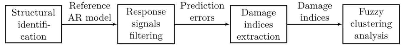
This chapter presents the development of a damage detection technique for a composite plate under series of loading. By using measured response signals, a reference AR model is identified and the separation of effects is performed by a fuzzy clustering method, as outlined in figure 1.
Figure 1 – Overview of the effect separation procedure.
Structural
identifi-cation
Response signals filtering
Damage indices extraction
Fuzzy clustering
analysis Reference
AR model
Prediction errors
Damage indices
Source: Created by the author.
3.1
Experimental Setup
The following experimental tests were performed in Stanford University, Department of Aeronautics & Astronautics – Structures and Composites Laboratory, by Professor Dr. Vicente Lopes Júnior on a composite structure provided by NASA. The data from this test was already processed in Lopes Jr and Chang (2012) showing satisfactory separation of effects with the use of artificial neural network. The aim of this experiment is to use a Lamb wave based method to study the behavior of a structure through a series of loads. Sensor measurements were taken through two SMART® piezoelectric (PZT) sensor patches bonded to the surface of a thin rectangular composite plate as seen in figure 2. Each sensor has six PZT transducers which can act as both actuators and sensors. A pitch catch measurement mode was chosen so the top layer was arbitrary set to excite the structure (actuators) while the bottom one was used as sensors (figure 2(a)).
ACESS® software with a sampling rate of 12 MHz1. The excitation signal chosen was a five peak Gaussian tone-burst with actuation frequency of 300 kHz. This frequency generates a S0 packet, with an acceptable level of dispersion (figure 3(c)), which is sensitive to the kind of damage tested, proven by many theoretical and experimental works (TAN et al., 1995; LEMISTRE; BALAGEAS, 2001; TOYAMA; TAKATSUBO, 2004; HU et al., 2008). Experimental signals for the undamaged structure (reference condition) are shown in figure 3(a)-(b). Figure 4 shows response signals for different conditions of the structure in the time interval from 55 to 75µsec in which the S0 packet is located.
Figure 2 – Composite structure coupled with two Smart® PZT sensor patches.
(a) Actuators and sensors in detail. (b) Schematic representation of the composite structure attached to the MTS.
Source: (a) Lopes Jr and Chang (2012); (b) Created by the author.
Several sets of experiments were performed to collect data from different load conditions. Although all available paths have been measured, only path 3-9 was used in order to minimize possible reflections caused by corners which could affect the following methodology for damage detection. The loading series were applied through a MTS®2 in three different days (figure 2(b)). In the first day the load ranged from 0 to 4.0 kip3, as shown in table 1, column 1 and 2. After these tests, X-ray showed that there was no damage in the structure. In the second day, the load ranged from 0 to 7.0 kip, column 3 and 4. Initial delamination began in approximately 5.0 kip. The last set of tests was carried out until the rupture, column 5 and 6. The rupture occurred in approximately 10.8 kip.
1More information about the acquisition softwre at:
http://www.acellent.com/blog1/products/ software/
2
Material Test System – equipment capable of applying controlled levels of load and/or temperature.
Figure 3 – Reference signals and dispersion curves for the composite structure. Am p lit u d e (V) Time (µs)
40 80 120 160
−50 −25 0 25 50
(a) Input signal for the undamaged structure.
Am p lit u d e (V) Time (µs)
40 80 120 160
−2 −1 0 1 2
(b) Output signal for the undamaged structure.
Frequency (kHz) P h as e ve lo ci ty (k m /s )
100 200 300 400 500
0 2 4 6
(c) Dispersion curves for the composite coupond
( S0 packet, A0 packet).
Source: Created by the author.
Figure 4 – Response signals under loading effect.
Am p li tu d e (V) Time (µs)
60 65 70 75
−1 −0.5
0 0.5
1
(a) Signals for the first loading series ( test
1, test 5, test 9, test 10).
Am p li tu d e (V) Time (µs)
60 65 70 75
−1 −0.5
0 0.5
1
(b) Signals for the second loading series ( test
11, test 15, test 19, test 22).
Table 1 – Test conditions (highlighted cells referring to unloaded condition).
Test Load Test Load Test Load Number (kip) Number (kip) Number (kip)
1 0 11 0 23 0
2 0.5 12 1.0 24 1.0
3 1.0 13 2.0 25 2.0
4 1.5 14 3.0 26 3.0
5 2.0 15 4.0 27 4.0
6 2.5 16 4.5 28 5.0
7 3.0 17 5.0 29 6.0
8 3.5 18 5.5 30 7.0
9 4.0 19 6.0 31 7.5
10 0 20 6.5 32 8.0
21 7.0 33 8.5
22 0 34 9.0
35 9.5 36 10.0 37 10.5 Source: Created by the author.
3.2
Extraction of Damage Indices
The ability to segregate data relies on the signal features which are extracted by damage indices. Thus, the chosen indices must provide enough information making possible the separation of the distinct effects that the structure is subjected. This work combines information obtained through time and frequency domain indices. Initially an AR model is created in order to reproduce the structure’s response for the reference (undamaged) condition4:
A(q)yref(k) =eyref(k) (1)
where yref(k) is the estimated response signal as a function of the discrete samplesk and
A(q) is a polynomial identified for the reference condition in order to monitory unknown
condition signals. The previous parameter is a function of the shift operator q whose
of order na is obtained by the computation of the Akaike’s information criterion (AIC)
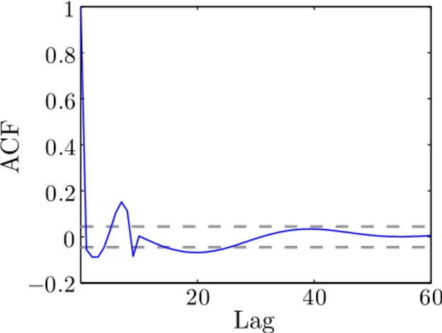
leading to a suitable value of 10. Then the model was validated with a certification signal – measurement 10 – with the same reference conditions (table 1). Certification was successful since an excellent fit percentage of 99.9% was obtained with the direct comparison of both signals (figure 5(a)). Additionally, an adequate level of residues in the response was
verified with the calculation of the autocorrelation function (ACF) converging to a 10% confidence interval as the lags increase which ensures the model’s ability to reproduce the structure’s behavior (figure 5(b)).
Figure 5 – Validation of the reference AR model.
Am p lit u d e (V) Time (µs)
40 80 120 160
−2 −1 0 1 2
(a) Direct comparison between the certification sig-nal (solid black line ) and the adjusted signal (dashed blue line ) with a fit percentage of 99.9.
A
C
F
Lag
20 40 60
−0.2
0 0.2
0.4
0.6
0.8
1
(b) Residue evaluation of adjusted response converg-ing to the confidence interval of 10% as the past samples (lags) increase.
Source: Created by the author.
The prediction error e(k) is related to the amount of the original response which is
not represented by the model. It is important to note that despite of the ideal random behavior expected for the prediction error to ensure a good system’s identification, in the present processing this parameter showed a deterministic behavior very similar to the response signals (figure 6). This was intentionally done so all effects acting on the structure besides load and damage were accounted in the model enabling the damage indices to be extracted directly from this parameter.
It is known that the change of the wave propagation is directly associated to material alterations due to varying operational and environmental conditions and/or the presence of damage5. Thus, it is possible to observe that the prediction errors suffered a leftward shift and amplification with the increase of tensile load. Also, the interruption of this pattern is verified between tests 15-19. This abrupt behavior change indicated that the handling of measurement variability sources could be performed by the application of a statistical model for the separation of effects without requiring any compensation procedures6. Thereby, the structural investigation was carried by the extraction of damage indices.
5See APPENDIX A for more information about wave propagation. 6
Figure 6 – Prediction errors. Am p lit u d e ( µ V) Time (µs)
60 65 70 75
−400 −200 0 200 400
(a) Signals for the first loading series ( test
1, test 5, test 9, test 10).
Am p lit u d e ( µ V) Time (µs)
60 65 70 75
−400 −200 0 200 400
(b) Signals for the second loading series ( test
11, test 15, test 19, test 22).
Source: Created by the author.
Firstly, the γ index was applied on the prediction errors (LU; GAO, 2005): γ = σ(eunk)
σ(eref)
(2)
where σ(∗) is the standard deviation operator, eref and eunk are the prediction errors
for the reference and unknown conditions, respectively. Because this index is based on the standard deviation it is more sensitive to variations in amplitude. Next, the cross correlation deviation metric (CCDM) was calculated using the prediction errors as well (GIURGIUTIU, 2002):
CCDM =1−RRRRRRRR
RRRR RR
∑Nk=1(ek,ref−eref)(ek,unk−eunk)
√
∑Nk=1(ek,ref−eref)2
√
∑Nk=1(ek,unk−eunk)2
RRRR RRRR RRRR RR
(3)
wherek is referred to discrete samples,N indicates the range of values for the calculations.
As discussed in chapter 2, CCDM is less sensitive to variations in amplitude but capable of detecting phase shifts.
Besides the time domain analysis performed, a time-frequency domain analysis is carried by the extraction of the short-time Fourier transform (STFT) whose matrix provides the energy map7. Its decomposition using singular value decomposition generates diagonal matrix Σ which is sensitive to structural alteration. The trace index is obtained through
the sum of its diagonal terms:
T race=
N
∑
i=1
Σii (4)
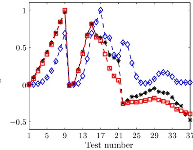
where Σii are the diagonal terms of matrix Σ. These three indices were normalized in
relation of their greatest value to generate a value range between 1 and -1 as presented in figure 7.
Figure 7 – Damage indices calculated for the clustering method (❩ –γ index, ◊ – CCDM, Ԃ – trace).
D
am
age
in
d
ex
val
u
e
Test number
1 5 9 13 17 21 25 29 33 37
−0.5
0 0.5
1
Source: Created by the author.
3.3
Cluster Analysis Results
The three damage indices calculated for the 37 load conditions, presented in table 1, were used in the separation performed by fuzzy c-means8 (figure 7) which is explained in APPENDIX D. The number of clusters is an unknown information, but it is crucial to the adequate classification. In the present procedure, the number of clusters was set as five – undamaged or reference condition, two levels of load and two levels of damage – mainly because of the knowledge of the effects that acted on the structure throughout the experiment. This choice can be a issue in cases where not all the sources of measurement variability are known.
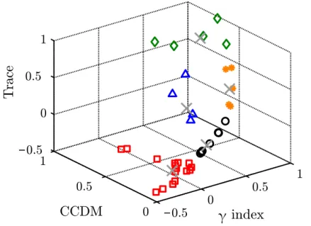
The result of the fuzzy clustering classification is showed in figure 8 in which it is possible to see that the representation of effects was well described. Due to the experimental
configuration, it is expected that the structure goes from a reference condition to increased load conditions. Despite the fact that loads up to 1.5 kip were classified into the reference cluster, the fuzzy clustering method confirmed no damage was imposed to the structure on the first load series, as seen in figure 9. Besides, the increasing load effect discussed before was verified. Damage was detected by the X-ray on the second load series around measurement 17 (5.0 kip), which is evidenced by the close classification at measurement 19 (6.0 kip). This fact confirms the accuracy of fuzzyc-means for damage detection.
Figure 8 – Three dimensional distribution of damage indices with cluster division (
○
– class 1, △ – class 2, ◊ – class 3, ❩ – class 4, Ԃ – class 5,×
–class center).
Source: Created by the author.
Moreover, since damage permanently changes the structure, no other undamaged condition is verified after damage is first detected (figure 9). Also, the cumulative effect of damage is captured as the classification goes from low damage to high damage definitively. Finally, imprecision in the classification can be related to the limited amount of data and operational condition diversity.
3.4
Conclusion
justified by their simple implementation and certification. Besides the two indices based on time domain analysis, spectrogram parameters are used in a fuzzy clustering method as well. This procedure successfully separated load effects from damage effects resulting in a reliable damage detection. Thus, the proposed approach is a robust unsupervised damage detection method that can be used in applications in which operational and environmental conditions play an important issue.
Figure 9 – Percentage results of fuzzy c-means classification: reference (Ref), low load (LL), high load (HL), low damage (LD) and, high damage (HD).
0 50 100
R
ef
L
L
0 50 100
H
L
0 50 100
L
D
0 50 100
H
D
Test number
1 5 9 13 17 21 25 29 33 37 0
50 100
Source: Created by the author.
4
Damage Prognosis based on
Coefficient Extrapolation
In this chapter a damage detection procedure with statistical confidence is carried using statistical process control. Also, a damage prognosis strategy is developed in order to forecast damage evolution in an aluminum plate subjected to a localized progressive mass loss. The prediction is based on the extrapolation of coefficients from identified structural conditions to create theoretical predictive models. This procedure is outlined in figure 10.
Figure 10 – Overview of damage detection associated to prognosis procedure.
Structural identification for damage detection Response signals filtering Damage index extraction Calculation of thresholds Structural identification for damage prognosis Coefficient extrapolation Future condition predicted Reference AR model Prediction errors Damage indices Structural conditions identified Series of ARX models Theoretical predictive ARX model
Source: Created by the author.
4.1
Experimental Setup
The present experimental tests were carried in CPqD1, Laboratory of Mechanical Tests, on a 1.6 mm thick aluminum plate coupled with six piezoelectric (PZT) patches (figure 11(a)). The structure was clamped at both ends in order to reduce measurement interference and kept at controlled room temperature (23± 3 °C), as showed in figures 11(b) and 12. A pitch-catch measurement mode was chosen with PZT 5 as actuator and PZT 2 as sensor. Data generation and acquisition was performed by a National
1
Instruments® PXI module and controlled by LabVIEW® software with a sampling rate of 10 MHz and an acquisition time window of 1.5 ms. The structure was excited by a five peak Gaussian tone-burst with 10 Vpp of amplitude and actuation frequency of 150 kHz
to guarantee damage detectability2 (figure 13(a)-(b)). This frequency generates an A0 packet3 of 930 m/s (figure 13(c)) with around 6 mm of wavelength which is located at the time window from 200 to 230 µs.
Figure 11 – Aluminum plate and the generation and acquisition system.
(a) Aluminum plate and its dimensions (dashed circle indicating damage location).
(b) Schematic representation of the aluminum plate.
Source: Created by the author.
Figure 12 – Experimental setup for damage prognosis.
(a) Aluminum plate coupled with six Piezo Sys-tems® PZT sensor patches.
(b) Data generation and aquisition system and plate support.
Source: Created by the author.
Two series of 10 signals were measured in distinct periods for each case studied for repeatability evaluation, as presented in table 2, with each acquired signal being a mean
2See APPENDIX A for more information about wave propagation.
of 10 signals. The response signals were normalized to produce zero mean and unitary standard deviation as a requirement for the following statistical methodology developed for damage detection (figure 14).
Figure 13 – Reference signals and dispersion curves for the aluminum plate.
Am p lit u d e (V) Time (µs)
500 1000 1500
−5 −2.5
0 2.5
5
(a) Input signal for the undamaged structure.
Am p lit u d e (m V) Time (µs)
500 1000 1500
−12 −6 0 6 12
(b) Output signal for the undamaged structure.
P h as e ve lo ci ty (k m /s )
Frequency × thickness (MHz×mm)
0.5 1 1.5 2 2.5
1 2 3 4 5 6
(c) Dispersion curves for the aluminum: ∗– S0 mode;+– A0 mode.
Source: Created by the author.
Table 2 – Sequence of measurements.
Condition tested Test number Damage depth (mm) Thickness reduction (%)
Reference 1 - 20 0 0
Damage 1 21 - 40 0.10 6.25
Damage 2 41 - 60 0.20 12.50
Damage 3 61 - 80 0.30 18.75
Damage 4 81 - 100 0.40 25.00
Source: Created by the author.
must be greater than half size of the wavelength generated (LEE; STASZEWSKI, 2003). This procedure was carried in the same face as the PZTs were bonded to the plate in an attempt to reproduce the effects of corrosion, which often affects aircraft structures and is hard to detect in inaccessible areas (figure 15).
Figure 14 – Normalized response signals in the time window from 200 to 230 µs corresponding to the first antisymmetric wave mode – A0 ( test
number 1, test number 21, test number 41, test number 61, test number 81).
Am
p
lit
u
d
e
(V)
Time (µs)
210 220 230
−6.4
−3.2
0 3.2
6.4
Source: Created by the author.
4.2
Damage Detection
The first of the two step identification was based on the estimation of a reference AR
model to provide a parametrization of the undamaged structural condition4. In this sense,
model identification and validation were performed using the first two signal responses, respectively (test numbers 1-2), since at this point the structure was considered to be undamaged (reference state). The model order determination was guided by the AIC index but also to ensure that the prediction errors would be able to carry information about damage, enabling the detection (figure 16). Thus, to meet such requirements, a suitable value for the reference model order was 2, leading to a satisfactory validation presented in figure 17.
Figure 15 – Apparatus for the creation of a controlled damage with progressive depth.
(a) Buehler® Electromet 4 electrolytic polisher composed of an electric circuit and an acid so-lution pump capable to produce controlled mass loss.
(b) Structure under electrolytic polishing .
(c) Resulting localized damage in detail to simulate
corrosion. (d) Damage depth measurement by a Starret® 2900electronic indicator.
Source: Created by the author.
Figure 16 – AIC index and prediction errors of the reference AR model for damage detection.
AI
C
in
d
ex
Order value - na
2 4 6 8 10
−25 −20 −15 −10 −5
0
(a) AIC index for the reference AR model.
Am
p
li
tu
d
e
(m
V)
Time (µs)
210 220 230
−8 −4 0 4 8
(b) Prediction errors ( test number 1,
test number 21, test number 41,
test number 61, test number 81).
Theγ index was used as the damage index due to its better sensitivity to variations in
amplitude since data dispersion is expected in the prediction errors when response signals of damaged conditions are filtered by the reference AR model. This index is defined as (LU; GAO, 2005):
γN =
σ(eN)
σ(eNref)
(5)
where N is the test number and the subscript ref refers to the position of the reference
indices with Nref =1,2,3,Ȃ,10 in this case generating 10 indices per test number, as
presented in figure 18(a).
Figure 17 – Validation of the reference AR model for damage detection.
Am p lit u d e (V) Time (µs)
210 220 230
−6.4
−3.2
0 3.2
6.4
(a) Direct comparison between the certification sig-nal (solid black line ) and the adjusted signal (dashed blue line ) with a fit percentage of
99.9.
A
C
F
Lag
10 20 30 40 50
−1 −0.5
0 0.5
1
(b) Residue evaluation of adjusted response converg-ing to the confidence interval of 10% as the past samples (lags) increase.
Source: Created by the author.
The thresholds for damage occurrence are defined by the computation of the control chart X-bar using the mean γ index value denoted by ¯γ (figure 18(b)). To do so, only
first 10 indices calculated were employed – the other 10 signals (test numbers 11-20 of the reference condition, for example) were kept to verify measurement variability and the occurrence of false indications of damage. The first step is the rearrangement of the indices inm subgroups of size n, normally chosen to be 4 or 5 (MONTGOMERY, 1996):
[γ¯]i,j =
¯
γ1,1 ¯γ1,2 Ȃ ¯γ1,n
¯
γ2,1 ¯γ2,2 Ȃ ¯γ2,n
⋮ ⋮ Ȃ ⋮
¯
γm,1 γ¯m,2 Ȃ γ¯m,n
(6)
can be reasonable approximated by a normal distribution as a result of the central limit theorem (SOHN et al., 2000). Thus, the mean and the standard deviation of each subgroup is calculated fori=1,2,Ȃ, m:
Xi =µ(γ¯i,j) Si =σ(γ¯i,j) (7)
withµ(∗) and σ(∗) being mean and standard deviation, respectively. Next, the central
line (CL) is obtained with the following expression:
CL=µ(Xi) (8)
Since data dispersion is expected for damaged conditions, only the upper control limit (UCL) is used as the threshold for damage detection:
U CL=CL+Zα/2
S
√
n (9)
where S=µ(Si). Due to measurement variability, the number of subgroupsn was defined
as 2 resulting in a subgroups of 5 elements. The term Zα/2 is the point in a normal distribution of zero mean and unitary standard deviation such that P(z >Zα/2)=α/2. In the present work a confidence interval of 99.73% was chosen leading toZα/2=3. Therewith, damage is detected when damage index value becomes greater than the threshold.
Figure 18 – Damage indices for the reference condition.
D am age in d ex Test number
2 6 10 14 18
0.98
0.99
1 1.01
1.02
(a) 10γinidces obtained for each test number.
D am age in d ex Test number
2 6 10 14 18
0.98
0.99
1 1.01
1.02
(b) Mean γ indices (∗) calculated for each test number and the respective threshold ( ). Source: Created by the author.
as damage became more severe. It is possible to obverse, for example, that damage index of test number 21 is located above the first threshold. At this moment damage is detected and a new threshold is obtained with the damage indices calculated with response signals from test numbers 21-30. These two identified conditions could enable the prediction of a third one as long as damage location and mass loss progression remain the same employing an adequate prognosis methodology.
Figure 19 – Damage indices (γ index) and thresholds for damage detection.
Threshold 1 Threshold 2 Threshold 3 Threshold 4 Threshold 5
D
am
age
in
d
ex
Test number
20 40 60 80 100
1 1.1
1.2
1.3
1.4
1.5
Source: Created by the author.
4.3
Damage Prognosis
As discussed before, the reference AR model for damage was estimated so the resulting prediction errors were able to carry information about damage progression. Similarly, the second step of the proposed structural identification is based on the modeling of response signals using autoregressive models with exognous inputs (ARX). This choice was guided due to the subtle changes verified in the response signals for the different conditions tested – predominantly phase shifts. Since ARX models consider the influence of the input signal to estimate the system´s output signal5, they are believed to better capture structural behavior exclusively for the condition they were created. This premise is crucial to ensure an adequate and unique identification of each structural condition tested enabling the prognosis of the structure´s future behavior by coefficient extrapolation.
The following procedure aims to forecast the structure’s behavior for a future condition taking into account past modeled conditions. Firstly, the input signal and the A0 packet of the response signals of test numbers 1-10 were used to create the first series ofstructural
identification models. Model validation was performed with signals from test number
11-20, so model 1 was validated with signals from test number 11 and so on. New of these series are created for the other damaged conditions detected as well, similarly to what was performed for the thresholds6.
The compromise to generate structural identification models “dedicated” only to the structural condition that they were created led to a order choice ofna=4 and nb=3. The
validation of the first ARX model created and validated with signals from test 1 and 11, respectively, is presented in figure 20 with an excellent fit percentage higher than 99% and a minimum level of residues in the response. All other structural identification models obtained for reference and damaged conditions presented similar results so their validation was omitted. Such capability was evaluated by the data dispersion in the prediction errors since this parameter should be minimized when both model and signals are related to the same condition, as discussed before. Each group of 10 structural identification models generated a set of prediction errors whose standard deviation was calculated. Their mean value and dispersion is presented in figure 21 evidencing the desired characteristic.
Figure 20 – Validation of the first structural identification model for the reference condition. Am p li tu d e (V) Time (µs)
210 220 230
−6.4
−3.2
0 3.2
6.4
(a) Direct comparison between the certification sig-nal (solid black line ) and the adjusted signal (dashed blue line ) with a fit percentage of
99.9. A C F ( × 10 − 5 ) Lag
10 20 30 40 50
−4 −2
0 2 4
(b) Residue evaluation of adjusted resposnse.
Source: Created by the author.
Structural prediction is accomplished by the extrapolation of ARX model coefficients
for the construction of theoretical predictive models. The basic assumption is that the damage evolution follows the same position and type. So, any new damage is inserted in the prediction. Since extrapolation aims to provide the value of a variable out of the range of known values, the trend of the preceding data is taken into account. However, the accuracy expected in the extrapolated coefficients is directly related to their behavior. A visual analysis evidences the complex evolution of coefficient values for the conditions modeled. Thereby, a preliminary approach is to only attempt to predict the response signal of the last damaged condition (0.4 mm of damage depth) taking into account all previous condition tested, as seen in figures 22 and 23. The best extrapolation result was obtained using the spline method7.
Figure 21 – Mean value and dispersion of standard deviations obtained from prediction errors generated by structural identification models of:
reference condition (test numbers 1-20); second damaged condition (0.2 mm of damage depth, test numbers 41-60); fourth damaged condition
(0.4 mm of damage depth, test numbers 81-100).
σ
(p
re
d
ic
ti
on
er
ror
)
(
µ
V)
Test number
20 40 60 80 100
10 15 20 25 30 35 40 45
Source: Created by the author.
The computation of these theoretical models follows the opposite way of the autore-gressive model estimation presented in APPENDIX B. Thus, the extrapolated coefficients form the polynomialsA(q) and B(q)and the predictive response can be estimated. The
success of the forecasting procedure is evidenced by figure 24 since the general decreasing behavior of the prediction errors’ standard deviation with the increase of damage severity was reproduced. Also, the predictive model generated prediction errors with levels of data dispersion similar to the structural identification models, as well. Therefore, this
7
methodology was able to produce a model to reasonable forecast structural behavior employing only measured data without the need of any physics or mathematical based models.
Figure 22 – Coefficient comparison for polynomial A(q): from structural
identification models; ∗– for theoretical predictive model (extrapolated).
a1
Damage depth (mm)
0 0.1 0.2 0.3 0.4
−4 −3.99 −3.98
(a) Coefficienta1.
a2
Damage depth (mm)
0 0.1 0.2 0.3 0.4
5.96 5.97 5.98 5.99 6 6.01 6.02
(b) Coefficienta2.
a3
Damage depth (mm)
0 0.1 0.2 0.3 0.4
−4.05 −4.04 −4.03 −4.02 −4.01 −4 −3.99 −3.98
(c) Coefficienta3.
a4
Damage depth (mm)
0 0.1 0.2 0.3 0.4
1 1.01 1.02
(d) Coefficienta4. Source: Created by the author.
because of their exclusive dependence on the system’s response without a clear physical link.
Figure 23 – Coefficient comparison for polynomialB(q): from structural
identification models; ∗– for theoretical predictive model (extrapolated).
b1 ( × 10 − 3 )
Damage depth (mm)
0 0.1 0.2 0.3 0.4
−0.05 0.95 1.95 2.95 3.95
(a) Coefficientb1.
b2 ( × 10 − 3 )
Damage depth (mm)
0 0.1 0.2 0.3 0.4
−8 −7 −6 −5 −4 −3 −2 −1 0 1
(b) Coefficientb2.
b3 ( × 10 − 3 )
Damage depth (mm)
0 0.1 0.2 0.3 0.4
0 1 2 3 4
(c) Coefficientb3. Source: Created by the author.
4.4
Conclusion
and 91-100 – last damaged condition). Finally, the statistical distribution of the damage indices could be evaluated to ensure that normal distribution assumption is accepted or the use of other types of data distribution is justified.
Figure 24 – Comparison of the mean value and dispersion of standard deviations obtained from prediction errors generated by the structural identification models for the fourth damaged condition ( 0.4 mm of damage depth, test numbers 81-100) and the absolute value of this parameter
generated by the theoretical predictive model (∗).
σ
(p
re
d
ic
ti
on
er
ror
)
(
µ
V)
Test number
20 40 60 80 100
10 15 20 25 30 35 40 45
Source: Created by the author.
Moreover, because of the complex behavior of the identified ARX models’ coefficients, a preliminary damage prognosis technique was attempted in order to forecast the structure’s behavior. This strategy satisfactorily predicted the structure’s dynamic response for a damage of 0.4 mm o depth taking into account four previous structural conditions and using the data dispersion verified in the prediction errors as the parameter of evaluation.
5
Final Remarks
In this chapter, the main conclusions achieved in this work are discussed. Also, suggestions for future research are presented.
5.1
Conclusion
This work studied the influence of operational and environmental conditions on damage detection with the creation of a monitoring method capable of separating the effects of loading from those of damage. It was evidenced that this topic is a crucial issue to become SHM suitable for real world applications. Additionally, damage prognosis was investigated and a primary technique was developed. In this sense, the main conclusions provided by the review of relevant works presented in chapter 2 are listed below:
• A feasible strategy to perform SHM is to develop techniques based only on time signal processing together with statistical models;
• Compensation procedures are suitable in order to separate the effects of undesirable factors, such as temperature and load, from the effects of damage in an early stage of a monitoring technique;
• Unsupervised learning algorithms are preferred since only data from the undamaged structure for their training. Also, their automatic nature and relatively simple development makes them attractive for on-board wireless applications;
• Damage prognosis is a natural evolution of SHM because of its capacity to optimize the useful life of a structure;
• To do so, it is fundamental to have a predictive model to track the changes associated to damage evolution.