Physical and Structural Improvements in the Stellar Evolutionary Code ATON2.3
Nat´alia Rezende Landin
NAT ´ALIA REZENDE LANDIN
Physical and Structural Improvements in the
Stellar Evolutionary Code
ATON2.3
Thesis submitted to UNIVERSIDADE FEDERAL DE MI-NAS GERAIS as a partial requirement for obtaining the Ph.D. degree in Physics
Concentration Area: ASTROPHYSICS
Advisor: Dr. Luiz Paulo Ribeiro Vaz (UFMG)
Co-Advisor: Dr. Luiz Themystokliz Sanctos Mendes (UFMG)
International Collaboration: Drs. Francesca D’Antona and Paolo Ventura (Osservatorio Astronomico di Roma, Italy)
Departamento de F´ısica - ICEx - UFMG
Agradecimentos
Agrade¸co sinceramente `as seguintes pessoas e institui¸c˜oes que contribuiram para a reali-za¸c˜ao deste trabalho:
- a Deus pela oportunidade de trabalhar fazendo o que gosto;
- aos meus pais, Eust´aquio e Lia, pelo amor, carinho, dedica¸c˜ao e por desempenharem t˜ao bem o dif´ıcil papel de pais;
- aos meus irm˜aos Rodrigo, Randal e Nardelle pelo apoio, companheirismo e amizade;
- `as minhas sobrinhas Isabela e Ana Fl´avia por preencherem nossa casa e nossas vidas com suas alegrias;
- ao Dr. Luiz Paulo (UFMG) pela orienta¸c˜ao, incentivo e amizade durante todo o curso;
- ao Dr. Luiz Themystokliz (CPDEE) pela co-orienta¸c˜ao e colabora¸c˜ao ao longo de todo o trabalho;
- aos meus co-orientadores italianos, Dra. Francesca D’Antona e Dr. Paolo Ventura
Osservatorio Astronomico di Roma), n˜ao somente pela enorme contribui¸c˜ao ao tra-balho, mas tamb´em pela hospitalidade durante minha estadia na It´alia;
- aos professores e amigos do Laborat´orio de Astrof´ısica;
- a todos os meus amigos;
- aos membros da banca examinadora pelas cr´ıticas construtivas feitas a este trabalho.
- aos funcion´arios do Departamento de F´ısica da UFMG, pela contribui¸c˜ao anˆonima;
- `a CAPES, pelo apoio financeiro dado atrav´es de bolsas de estudos tanto no Brasil quanto no exterior;
Acknowledgements
I thank sincerely the following persons and institutions that contributed to the accom-plishment of this work:
- God for the opportunity to work doing what I like to do;
- my parents, Eust´aquio e Lia, for their love, care, dedication and for performing so well the hard role of being parents;
- my brothers Rodrigo, Randal and my sister Nardelle for their constant support, company and friendship;
- my nieces, Isabela and Ana Fl´avia, for filling our home and lives with their joy;
- Dr. Luiz Paulo (UFMG) for the orientation, support and friendship during all the course;
- Dr. Luiz Themystokliz Sanctos Mendes (CPDEE) for the co-orientation and collab-oration during all these years;
- my italian co-advisors, Dr. Francesca D’Antona and Dr. Paolo Ventura (Osservatorio Astronomico di Roma) not only for the enourmous contribution to the work, but also for their hospitality during my stay in Italy;
- my friends and teachers of the Astrophysics Lab;
- all my friends;
- the judging committee for the constructive critic given to this work;
- the staff of Physics Department - UFMG - for their anonymous contributions;
- CAPES for the financial support through scholarships during the whole course, including my stage in Italy;
Contents
1 Introduction 1
2 Structural Changes in the Stellar Evolutionary Code ATON 2.3 9
2.1 Implementation of the structural changes . . . 9
2.2 The importance of the checkpoint mechanism . . . 11
3 Internal Structure Constants 12 3.1 Apsidal motion . . . 13
3.1.1 Relativistic Effects . . . 15
3.1.2 Effects of a third body . . . 15
3.1.3 Effects of interstellar medium . . . 16
3.2 Equilibrium configuration of stars . . . 16
3.3 Internal structure constants for spherically symmetric configurations . . . . 18
3.4 The Kippenhahn & Thomas’s formulation . . . 19
3.5 Tidal and/or rotational distortions on the equilibrium structure of stars . . 21
3.5.1 Rotational distortion . . . 22
3.5.2 Tidal distortion . . . 25
3.5.3 Interaction between rotation and tides . . . 29
3.5.4 Rotational inertia . . . 32
3.6 Results . . . 36
3.6.1 Internal structure constant for single non-rotating stars . . . 36
3.6.2 Internal structure constants for non-rotating stars in binary systems 37 3.6.3 Internal structure constants for single rotating stars . . . 38
3.6.4 Internal structure constants for rotating stars in binary systems . . 38
3.7 Discussion . . . 39
3.7.1 Comparison with other works . . . 42
3.8 Comparison between theory and observations . . . 44
3.9 Conclusions . . . 50
4 Theoretical Values of the Rossby Number 52 4.1 Introduction . . . 52
4.2 The solar dynamo . . . 54
4.3 Input physics . . . 55
4.4 Rossby number calculations . . . 56
5 Non-Gray Atmospheres 63
5.1 Convection treatment in the atmosphere . . . 65
5.2 Non-gray boundary conditions in theATON code . . . 67
5.3 Applications of the new rotating non-gray version of ATON2.4 code . . . 68
5.3.1 An overview of theoretical pre-main sequence models . . . 68
5.3.2 An overview on the observational data of ONC . . . 69
5.3.3 Physical input of the models used to analyze the ONC stars . . . . 70
5.3.3.1 Boundary conditions . . . 70
5.3.3.2 Convective treatment . . . 71
5.3.3.3 The role of convection coupled with the non-gray atmo-spheres . . . 72
5.3.3.4 Rotation and initial angular momentum . . . 73
5.3.3.5 The lithium depletion . . . 75
5.3.4 Data from the literature - ONC . . . 77
5.3.5 Derivation of masses and ages . . . 77
5.3.6 Comparison with gray models . . . 79
5.3.7 Stellar rotation in the ONC . . . 80
5.3.7.1 The dichotomy in period distribution for different mass ranges . . . 80
5.3.8 Disk locking and the disk lifetime . . . 81
5.3.9 An alternative view: the role of the magnetic field . . . 84
5.3.10 A constant angular momentum evolution? . . . 85
5.3.11 The X-ray emission of the ONC stars . . . 86
5.3.12 Conclusions . . . 87
6 Final Remarks 89 6.1 General conclusions . . . 89
6.2 Future works . . . 92
6.2.1 Approximations to the meridional circulation velocity . . . 92
6.2.2 Rotation-induced diffusion of chemicals . . . 92
6.2.3 Effects of a µ-gradient . . . 93
6.2.4 Interaction between rotation and magnetic fields . . . 94
7 S´ıntese do trabalho em l´ıngua portuguesa 96 7.1 Introdu¸c˜ao . . . 96
7.1.1 Tema de pesquisa . . . 96
7.1.2 Relevˆancia e justificativa do tema de pesquisa . . . 97
7.2 Mudan¸cas estruturais no c´odigo ATON2.3 . . . 99
7.2.1 Implementa¸c˜ao das mudan¸cas estruturais . . . 99
7.2.2 Importˆancia do “checkpoint”, ou ponto de controle . . . 99
7.3 Distor¸c˜oes na estrutura de equil´ıbrio devido `as for¸cas rotacionais e de mar´e 100 7.4 C´alculo te´orico do N´umero de Rossby . . . 102
7.5 Inclus˜ao de atmosferas n˜ao-cinza . . . 104
7.6 Conclus˜oes . . . 106
7.7 Trabalhos futuros . . . 108
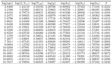
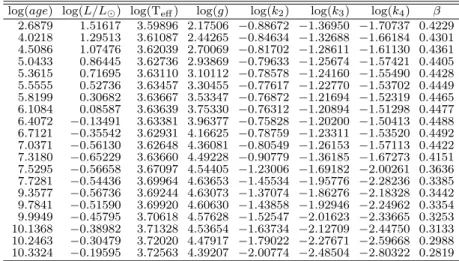
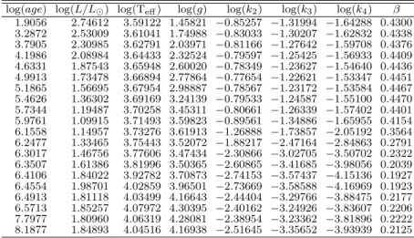
A Pre-main sequence stellar evolutionary models including internal
struc-ture constants 114
A.1 Standard models: single non-rotating stars . . . 114
A.2 Binary models: non-rotating stars in binary systems . . . 122
A.3 Rotating models: single rotating stars . . . 130
A.4 Rotating binary models: rotating stars in binary systems . . . 138
B Published Papers 147 B.1 Theoretical values of the Rossby Number for low-mass, rotating pre-main sequence stars . . . 147
List of Figures
1.1 H-R diagram. . . 2
2.1 The functioning of the checkpoint mechanism . . . 10
3.1 Rotational and tidal distortion . . . 17
3.2 Geometric configuration for the Roche potential. . . 19
3.3 Evolutionary tracks for standard and distorted models. . . 40
3.4 log(k2) vs. age for standard and distorted models. . . 41
3.5 log(k2) vs. age for different (X,Z) and log(kj) x log (M) for ZAMS models . 42 3.6 log(β) x log (M) and log(kj) x log(β) for ZAMS models . . . 42
3.7 Temporal evolution of stellar radius for different models. . . 43
3.8 Stellar radii and TR vs. age for EK Cep components. . . 45
3.9 EK Cep components and corresponding mass tracks in the HR diagram. . . 47
3.10 EK Cep components and corresponding mass tracks in the log(g) vs. log (Teff) plane. . . 48
3.11 Temporal evolution of Li content and log(k2) for EK Cep components. . . . 49
4.1 Chromospheric Ca II flux vs. Ro. . . 53
4.2 Azimuthal and meridional fields. . . 55
4.3 The ω-effect. . . 55
4.4 Prot vs. age. . . 56
4.5 Local τc vs. age. . . 57
4.6 Global convective turnover time vs. age. . . 58
4.7 Dynamo number vs. age. . . 58
4.8 τc (global) vs. Teff and τc vs. Prot for some isochrones. . . 59
4.9 Prot vs. Teff and R−o2 vs. Prot for some isochrones. . . 60
4.10 Ro−2 vs. T eff for some isochrones. . . 61
5.1 Non-gray evolutionary tracks and isochrones forα=1.0, 2.0 and 2.2. . . 70
5.2 Overadiabaticity and mass fraction where (∇ − ∇ad)>10−4 vs. luminosity. 73 5.3 Comparison between convection and non-grayness effects on the tracks. . . 74
5.4 The temporal evolution of lithium depletion. . . 75
5.5 Lithium depletion vs. Teff. . . 76
5.6 Mass and age histograms for the ONC stars. . . 78
5.7 Age distributions for masses lower and higher than Mtr. . . 79
5.8 The period histogram of all observed ONC objects. . . 80
5.9 Period histograms as function of mass. . . 80
5.11 The mass distribution of the early fast rotators and slow rotators. . . 83
5.12 The observed infrared excess as function of mass. . . 83
5.13 Fig. 1 from Barnes 2003 . . . 85
5.14 Temporal evolution of periods for α=1.0, 2.0 and 2.2. . . 86
5.15 LX luminosity (ergs/s) plotted against mass. . . 87
List of Tables
3.1 ISC and gyration radii for ZAMS standard models. . . 37
3.2 ISC and gyration radii for ZAMS tidal distorted models. . . 37
3.3 ISC and gyration radii for ZAMS rotating models. . . 38
3.4 ISC and β for ZAMS rotationally and tidally distorted models. . . 38
3.5 The comparison between the available log (k2). . . 44
3.6 Absolute dimensions of EK Cep. . . 45
3.7 Summary of the apsidal motion related quantities. . . 50
4.1 Isochrones for all models. . . 62
5.1 Li abundances at 108yr for some models. . . 75
5.2 Comparison between gray and non-gray models. . . 81
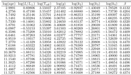
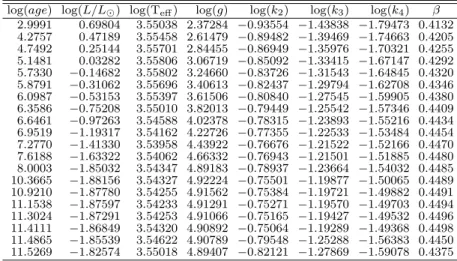
A.1 ISC and gyration radii for 0.09 M⊙ pre-MS standard models. . . 114
A.2 ISC and gyration radii for 0.10 M⊙ pre-MS standard models. . . 115
A.3 ISC and gyration radii for 0.20 M⊙ pre-MS standard models. . . 115
A.4 ISC and gyration radii for 0.30 M⊙ pre-MS standard models. . . 115
A.5 ISC and gyration radii for 0.40 M⊙ pre-MS standard models. . . 116
A.6 ISC and gyration radii for 0.50 M⊙ pre-MS standard models. . . 116
A.7 ISC and gyration radii for 0.60 M⊙ pre-MS standard models. . . 116
A.8 ISC and gyration radii for 0.70 M⊙ pre-MS standard models. . . 117
A.9 ISC and gyration radii for 0.80 M⊙ pre-MS standard models. . . 117
A.10 ISC and gyration radii for 0.90 M⊙ pre-MS standard models. . . 117
A.11 ISC and gyration radii for 1.00 M⊙ pre-MS standard models. . . 118
A.12 ISC and gyration radii for 1.20 M⊙ pre-MS standard models. . . 118
A.13 ISC and gyration radii for 1.40 M⊙ pre-MS standard models. . . 118
A.14 ISC and gyration radii for 1.60 M⊙ pre-MS standard models. . . 119
A.15 ISC and gyration radii for 1.80 M⊙ pre-MS standard models. . . 119
A.16 ISC and gyration radii for 2.00 M⊙ pre-MS standard models. . . 119
A.17 ISC and gyration radii for 2.30 M⊙ pre-MS standard models. . . 120
A.18 ISC and gyration radii for 2.50 M⊙ pre-MS standard models. . . 120
A.19 ISC and gyration radii for 2.80 M⊙ pre-MS standard models. . . 120
A.20 ISC and gyration radii for 3.00 M⊙ pre-MS standard models. . . 121
A.21 ISC and gyration radii for 3.30 M⊙ pre-MS standard models. . . 121
A.22 ISC and gyration radii for 3.50 M⊙ pre-MS standard models. . . 121
A.23 ISC and gyration radii for 3.80 M⊙ pre-MS standard models. . . 122
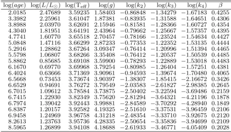
A.25 ISC and gyration radii for 0.10 M⊙ pre-MS tidal distorted models. . . 123
A.26 ISC and gyration radii for 0.20 M⊙ pre-MS tidal distorted models. . . 123
A.27 ISC and gyration radii for 0.30 M⊙ pre-MS tidal distorted models. . . 123
A.28 ISC and gyration radii for 0.40 M⊙ pre-MS tidal distorted models. . . 124
A.29 ISC and gyration radii for 0.50 M⊙ pre-MS tidal distorted models. . . 124
A.30 ISC and gyration radii for 0.60 M⊙ pre-MS tidal distorted models. . . 124
A.31 ISC and gyration radii for 0.70 M⊙ pre-MS tidal distorted models. . . 125
A.32 ISC and gyration radii for 0.80 M⊙ pre-MS tidal distorted models. . . 125
A.33 ISC and gyration radii for 0.90 M⊙ pre-MS tidal distorted models. . . 125
A.34 ISC and gyration radii for 1.00 M⊙ pre-MS tidal distorted models. . . 126
A.35 ISC and gyration radii for 1.20 M⊙ pre-MS tidal distorted models. . . 126
A.36 ISC and gyration radii for 1.40 M⊙ pre-MS tidal distorted models. . . 126
A.37 ISC and gyration radii for 1.60 M⊙ pre-MS tidal distorted models. . . 127
A.38 ISC and gyration radii for 1.80 M⊙ pre-MS tidal distorted models. . . 127
A.39 ISC and gyration radii for 2.00 M⊙ pre-MS tidal distorted models. . . 127
A.40 ISC and gyration radii for 2.30 M⊙ pre-MS tidal distorted models. . . 128
A.41 ISC and gyration radii for 2.50 M⊙ pre-MS tidal distorted models. . . 128
A.42 ISC and gyration radii for 2.80 M⊙ pre-MS tidal distorted models. . . 128
A.43 ISC and gyration radii for 3.00 M⊙ pre-MS tidal distorted models. . . 129
A.44 ISC and gyration radii for 3.30 M⊙ pre-MS tidal distorted models. . . 129
A.45 ISC and gyration radii for 3.50 M⊙ pre-MS tidal distorted models. . . 129
A.46 ISC and gyration radii for 3.80 M⊙ pre-MS tidal distorted models. . . 130
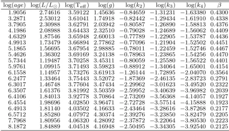
A.47 ISC and gyration radii for 0.09 M⊙ pre-MS rotating models. . . 130
A.48 ISC and gyration radii for 0.10 M⊙ pre-MS rotating models. . . 131
A.49 ISC and gyration radii for 0.20 M⊙ pre-MS rotating models. . . 131
A.50 ISC and gyration radii for 0.30 M⊙ pre-MS rotating models. . . 131
A.51 ISC and gyration radii for 0.40 M⊙ pre-MS rotating models. . . 132
A.52 ISC and gyration radii for 0.50 M⊙ pre-MS rotating models. . . 132
A.53 ISC and gyration radii for 0.60 M⊙ pre-MS rotating models. . . 132
A.54 ISC and gyration radii for 0.70 M⊙ pre-MS rotating models. . . 133
A.55 ISC and gyration radii for 0.80 M⊙ pre-MS rotating models. . . 133
A.56 ISC and gyration radii for 0.90 M⊙ pre-MS rotating models. . . 133
A.57 ISC and gyration radii for 1.00 M⊙ pre-MS rotating models. . . 134
A.58 ISC and gyration radii for 1.20 M⊙ pre-MS rotating models. . . 134
A.59 ISC and gyration radii for 1.40 M⊙ pre-MS rotating models. . . 134
A.60 ISC and gyration radii for 1.60 M⊙ pre-MS rotating models. . . 135
A.61 ISC and gyration radii for 1.80 M⊙ pre-MS rotating models. . . 135
A.62 ISC and gyration radii for 2.00 M⊙ pre-MS rotating models. . . 135
A.63 ISC and gyration radii for 2.30 M⊙ pre-MS rotating models. . . 136
A.64 ISC and gyration radii for 2.50 M⊙ pre-MS rotating models. . . 136
A.65 ISC and gyration radii for 2.80 M⊙ pre-MS rotating models. . . 136
A.66 ISC and gyration radii for 3.00 M⊙ pre-MS rotating models. . . 137
A.67 ISC and gyration radii for 3.30 M⊙ pre-MS rotating models. . . 137
A.68 ISC and gyration radii for 3.50 M⊙ pre-MS rotating models. . . 137
A.69 ISC and gyration radii for 3.80 M⊙ pre-MS rotating models. . . 138
A.70 ISC and β for 0.09 M⊙ pre-MS rotationally and tidally distorted models. . 138
A.72 ISC and β for 0.20 M⊙ pre-MS rotationally and tidally distorted models. . 139
A.73 ISC and β for 0.30 M⊙ pre-MS rotationally and tidally distorted models. . 139
A.74 ISC and β for 0.40 M⊙ pre-MS rotationally and tidally distorted models. . 140
A.75 ISC and β for 0.50 M⊙ pre-MS rotationally and tidally distorted models. . 140
A.76 ISC and β for 0.60 M⊙ pre-MS rotationally and tidally distorted models. . 140
A.77 ISC and β for 0.70 M⊙ pre-MS rotationally and tidally distorted models. . 141
A.78 ISC and β for 0.80 M⊙ pre-MS rotationally and tidally distorted models. . 141
A.79 ISC and β for 0.90 M⊙ pre-MS rotationally and tidally distorted models. . 141
A.80 ISC and β for 1.00 M⊙ pre-MS rotationally and tidally distorted models. . 142
A.81 ISC and β for 1.20 M⊙ pre-MS rotationally and tidally distorted models. . 142
A.82 ISC and β for 1.40 M⊙ pre-MS rotationally and tidally distorted models. . 142
A.83 ISC and β for 1.60 M⊙ pre-MS rotationally and tidally distorted models. . 143
A.84 ISC and β for 1.80 M⊙ pre-MS rotationally and tidally distorted models. . 143
A.85 ISC and β for 2.00 M⊙ pre-MS rotationally and tidally distorted models. . 143
A.86 ISC and β for 2.30 M⊙ pre-MS rotationally and tidally distorted models. . 144
A.87 ISC and β for 2.50 M⊙ pre-MS rotationally and tidally distorted models. . 144
A.88 ISC and β for 2.80 M⊙ pre-MS rotationally and tidally distorted models. . 144
A.89 ISC and β for 3.00 M⊙ pre-MS rotationally and tidally distorted models. . 145
A.90 ISC and β for 3.30 M⊙ pre-MS rotationally and tidally distorted models. . 145
A.91 ISC and β for 3.50 M⊙ pre-MS rotationally and tidally distorted models. . 145
Resumo
No presente trabalho investigamos alguns efeitos f´ısicos que acontecem na estrutura e evolu¸c˜ao estelar. Focalizamos nossa aten¸c˜ao em estrelas de baixa massa na pr´e-sequˆencia principal. Incluimos alguns efeitos f´ısicos no c´odigo de estrutura e evolu¸c˜ao estelar
ATON2.3, escrito pelo Dr. Italo Mazzitelli (1989) e posteriormente modificado pelo Dr. Luiz Themystokliz Sanctos Mendes (1999b) para adicionar os efeitos de rota¸c˜ao e redis-tribui¸c˜ao interna de momentum angular. Com o objetivo de economizar tempo computa-cional, introduzimos o mecanismo de parada de controle (checkpoint), que permite iniciar uma dada execu¸c˜ao em um est´agio de evolu¸c˜ao intermedi´ario, desde que os passos ini-ciais tenham sido devidamente registrados. Essas modifica¸c˜oes foram feitas juntamente com um controle completo de vari´aveis n˜ao inicializadas, precis˜ao e reestrutura¸c˜ao do programa, visando futuramente paralelizar o c´odigo. Introduzimos efeitos combinados de rota¸c˜ao e for¸cas de mar´e na configura¸c˜ao de equil´ıbrio das estrelas. Esses efeitos pertur-badores, contidos na fun¸c˜ao potencial total, desviam a forma da estrela da aproxima¸c˜ao esfericamente sim´etrica. Usamos o m´etodo de Kippenhahn & Thomas (1970), poste-riormente aperfei¸coado por Endal & Sofia (1976). `A fun¸c˜ao potencial obtida por esses autores, adicionamos termos relacionados a for¸cas de mar´e e outros relacionados `a parte n˜ao sim´etrica do potencial gravitacional devido `a distor¸c˜ao que tais for¸cas causam na figura da estrela. Seguindo essa aproxima¸c˜ao, corrigimos as equa¸c˜oes constitutivas a fim de obter uma configura¸c˜ao estrutural de uma estrela distorcida. Derivamos uma nova ex-press˜ao para a in´ercia rotacional de estrelas sob a a¸c˜ao de potenciais perturbativos devido `a rota¸c˜ao e for¸cas de mar´e. C´alculos de constantes de estrutura interna e raios de gira¸c˜ao foram inclu´ıdos no c´odigo tanto para para o caso os modelos sem distor¸c˜ao quanto para os distorcidos. Apresentamos, pela primeira vez na literatura, c´alculos de constantes de estrutura interna que se extendam at´e a pr´e-sequˆencia principal. V´arias trilhas evolutivas foram geradas com os novos modelos, incluindo as grandezas mencionadas acima. Os novos modelos foram testados atrav´es de dados observacionais das dimens˜oes absolutas, taxa de movimento apsidal e abundˆancia de l´ıtio das componentes do sistema bin´ario eclipsante EK Cephei. No presente trabalho, tamb´em apresentamos estimativas te´oricas do “convective turnover time”, τc, e N´umeros de Rossby, Ro, para estrelas com massas
Abstract
We have investigated some physical phenomena that take place in the stellar structure and evolution. Special attention was given to low-mass pre-main sequence stars. We have included the possibility of using non-gray atmosphere models in the boundary conditions, as well as the possibility of extracting information of some physical effects (like the internal structure constant and the Rossby number) in the stellar evolutionary codeATON2.3. The code was originally written by Dr. Italo Mazzitelli (1989) and further improved by Dr. Luiz Themyztokliz Sanctos Mendes (1999b) to take into account the effects of rotation and redistribution of angular momentum. In order to save computing time, we have introduced a checkpoint mechanism that allow starting the run in any step of evolution since previous computations had been registered. This modification was done together with a complete control for non-initialized variables, machine precision and restructuring, aiming a later implementation of parallel computation. We have introduced the effects of tidal forces combined with the rotational ones on the equilibrium configuration of the stars. These disturbing effects, all included in the total potential function, deviate the stellar configuration from sphericity. We have used the Kippenhahn & Thomas (1970) approximation, which was further improved by Endal & Sofia (1976). To the potential function obtained by the latter authors, we added both the terms related to the tidal potentials and those related to the non-symmetrical part of the gravitational potential due to the distortion of the star figure due to tidal forces. Following this approach, we correct the constitutive equations in order to obtain a stellar structure configuration of a distorted star. We dereived a new expression for the rotational inertia of tidally and rotationally distorted star. We included also calculations of internal structure constants and gyration radii, tabulating them for a serie of models. We presented, for the first time in the literature, calculations of the internal structure constant extended to the pre-main sequence. Our new models were tested against observations through the analysis of the evolutionary status of EK Cephei. We also present theoretical estimates of the convective turnover time, τc, and Rossby numbers, Ro, for rotating pre-main sequence solar-type
Chapter 1
Introduction
The physical processes occuring in the stellar interiors cannot be directly observed, except, perhaps, through the elusive neutrinos. The vast majority of the information we have about the conditions existing inside a star, comes from the light emitted by its atmosphere, what indirectly reflects the internal environment.
The stellar interior properties must be deduced from the observed features and from the laws that govern the stellar structure and evolution. Through a suitable combination of these laws in theoretical models, one can have an insight of the equilibrium configuration and of the temporal evolution of the stars.
There exist only few stellar features that can be directly observed. For a large number of stars, we have measurements of magnitudes (apparent and absolute) and color indexes. For the Sun and a relatively small number of components of binary systems, we have good determination of masses, radii and luminosities. Additional verifications in theories are provided by data obtained from asteroseismology, the study of the internal structure of stars through the interpretation of their pulsation periods, and from binary systems in which the line of apsides (the major axis of the orbit) presents a small rotation veloc-ity. This phenomenon depends on the stellar internal conditions and, therefore, provides information that can be used to control the stellar interior theories. Information about the chemical composition of the stellar surface can be achieved spectroscopically, and one can assume that the composition of the major part of the stellar interior is similar to that of the outer layers, at least for main sequence (MS) stars. On the other hand, giant stars have already processed part of the elements originally present in their interior, and the spectroscopic data can only provide reliable information about the surface chemical composition.
(usually referred to by the abbreviation H-R diagram or HRD; another form of it is also known as a Colour-Magnitude diagram, or CMD). It shows the relationship between absolute magnitude, luminosity, spectral classification, and surface temperature of stars. The diagram was developed independently by Ejnar Hertzsprung in 1911 and Henry Norris Russell in 1913 and represented a huge leap forward in understanding stellar evolution, or the “lives of stars”. From it, most of the peculiarities of stellar behavior can be studied. One of these, in particular, is that the stars are sitting along a well-defined band called MS, where the majority of stars are clustered in a region from the bottom right to the top left (see Fig. 1.1). The H-R diagram is the fundamental tool astronomers use to explore the birth and the death of stars. Although it began as a way to group information concerning the intrinsic characteristics of stars, it quickily became a tool to explore changes in stars as they age. It is used to define different types of stars and to match theoretical predictions of stellar evolution using computer models with observations of actual stars. It is then necessary to convert either the calculated quantities to observables, or the other way around, thus introducing an extra uncertainty.
The theoretical studies about the stellar interior are based in a set of equations that must be solved simultaneously, aiming to reproduce the observed stellar properties and to explain the internal structure of the stars. Such models treat the physical phenomena taking place inside a star by describing them through basic equations that govern the internal physical properties. The basis of the stellar structure theory was developed in the first part of the past century, when several important works were published, among which those of Chandrasekhar (1939) and Schwarzschild (1958) can be considered the fundamental ones.
The structure of a star can be described by a set of differential equations contain-ing variables like pressure, density, temperature, luminosity, etc. They are the so-called “constitutive equations”:
dP
dM = −
GM
4πr4 (1.1a)
dr
dM =
1
4πr2ρ (1.1b)
dL
dM = ǫ−T
∂S
∂t (1.1c)
dT
dM = −
GMT
4πr4P∇, ∇={∇rad,∇conv}. (1.1d)
This equations are respectively named equation of hydrostatic equilibrium, equation of continuity of mass, equation of conservation of energy and equation of transport of energy. Besides the set of Eqs. (1.1), it is also necessary to assume an equation of state of the material that form the star, an opacity law and an equation of energy generation to describe the stellar structure. Furthermore, some boundary conditions must be defined in order to match interior and atmosphere integrations. The theoretical models are built aiming the self consistent solution of these equations throughout the stellar radius, having the stellar mass and the initial chemical composition (and, eventually, some amount of rotation) as input parameters. A sequence of models of stellar structure in successive time intervals define a stellar “evolutionary track” in the HRD.
In the 1960’s, the construction of evolutionary models was stimulated by the introduc-tion of the relaxation method for the numerical solution of the differential equations that describe the stellar structure (Henyey, Forbes & Gould 1964). This method replaces the differential equations with a set of finite difference equations whose solution is carried out globaly and enables one to include time-dependent phenomena in a natural way. Also, the appearing of faster computers speeded up the improvement process of the models. Besides that, the knowledge of several other aspects of the stellar interiors, such as nu-cleosynthesis of elements (Clayton 1968) and more realistic opacity tables calculations (Cox & Stewart 1970), were important in bringing the models to a very well succeeded interpretation of a large part of intermediate mass stars in the MS phase.
approximations for the underlying physical phenomena. It is important to emphasize that, although some of the physical processes involved in the stellar theories have solid theoretical basis, the corresponding implementation in the models is, most of the times, a hard task. This is due to a series of problems, such as numerical accuracy and instability, mathematical complexity, computational time, and so on. A significant number of im-portant questions related to stellar structure and evolution is still under debate. A good example is turbulence, that is not well understood, yet. Many of these several open issues are discussed in some reference works. For example, the problem of the chemical mix-ing of elements was addressed by Goulpil & Zahn (1989); D’Antona & Mazzitelli (1984) discuss the lithium and berilium burning, Mihalas et al. (1988) treat the stellar equation of state; Canuto & Mazzitelli (1991) give some insight on the turbulent convection, and Kippenhahn & Thomas (1970) investigated the influence of rotation in the stellar evolu-tion. Some of these subjects, like rotation and turbulent convection, have already been implemented in the evolutionary models and presented promising results.
Regarding the star formation process, one believes that the stars are formed from clouds made up by the interstellar material. The chemical composition of a newborn star is similar to that of the cloud from which the star in question was formed. The total stellar mass is primarily determined in the formation process, although it can undergo some changes due to the residual accretion after the protostellar phase (Basri & Bertout 1989) and to outflows, which are mass loss processes due to magneto-rotationally driven winds (Hartmann & MacGregor 1982).
Star formation occurs as a result of the action of gravity on a wide range of scales, and different mechanisms may be important on different scales, depending on the forces opposing gravity. On galactic scales, the tendency of interstellar matter to condense under gravity into star-forming clouds is counteracted by galatic tidal forces, and star formation can occur only where the gas becomes dense enough for its self-gravity to overcome these tidal forces, for example in spiral arms (Larson 2003). On intermediate scales, turbulence and magnetic fields may be the most important effects opposing gravity, while on the small scales of individual prestellar cloud cores, thermal pressure becomes the most important force resisting gravitation. When the cloud core begins contracting, the centrifugal force associated with its angular momentum may eventually interrupt the collapse, leading to the formation of a binary or multiple star system. When a very small central region attains stellar density, the contraction is halted by the thermal pressure and a protostar forms and continues growing in mass by accretion. In this final stage of star formation, magnetic fields can become important by controlling gas accretion and outflows. These events characterize the pre-main sequence (pre-MS) evolutionary phase. As the thermodynamic conditions within a star become close to those suitable for the nuclear reactions ignition, these phenomena finish and the star approaches a far more stable configuration, called MS.
“burning” is almost completely consumed. As the more massive stars have higher central temperature, pressure and density, they process their nuclear Hydrogen faster than the lower mass stars, remaining less time in the MS. Therefore, the time spent by a given star in the MS phase, and, in general, in its evolution after that, is determined by its initial mass.
Depending on the stellar mass, other chemical elements can be processed in the stel-lar nucleus. The production of new elements, other than Helium (from H-burning), by nuclear reactions is called “nucleosynthesis”. Again, the stellar mass will determine what kind of reactions will take place in the central core of a star. Objects with less than 0.08M⊙, the so-called brown dwarfs, are not real stars because they never develop a
cen-tral temperature which is high enough to ignite Hydrogen burning. Instead, they release energy by gravitational contraction. The very low mass stars (between about 0.25 and 0.08 M⊙) are real fully convective stars that burn Hydrogen in their cores, via p-p chain,
so slowly that they will stay on the MS for a very long time (about 1012 years). Once
Hydrogen is burned out, the core collapes, but never reaches temperatures high enough to ignite Helium-burning. Such stars evolve directly to white dwarfs. One believes that the universe is so young that no very low-mass stars has had time to evolve off the MS, so this prediction is not really testable. Low mass stars (0.25<M/M⊙<1.2) have radiative
cores, so that the surrounding Hydrogen cannot be transported into the core where it can be burned. Instead, only the Hydrogen inilially present in the inner core, where the temperature is high enough, will be processed via p-p chain. When the Hydrogen is used up, the central core contracts gravitationally until the degeneracy halts the contraction. Eventually, the core will heat up until Helium can be ignited and, when this occurs, the star is in a giant phase. He-burning in degenerate core takes place explosively, in a pro-cess called “Helium Flash”. The changes produced by this propro-cess are very rapid and the physics involved becomes very difficult to be described approximately. Despite the difficulties involved in calculations of the He flash, the star certainly ends up in a stable configuration, where it burns Helium in the core and Hydrogen in a shell around it. This phase is called the “Horizontal Branch”. After Helium is used up in the core, He-burning shell takes place, but the star will not be able to burn any further element because it cannot get hot enough in the core, and it will move to the white dwarf region.
High mass stars (M>1.2 M⊙) have convective cores and, for this reason, a large amount
heavier nucleus by direct fusion is endothermic. Massive stars can reach a stage where they consist of shells of nuclear burning, with Fe production in the core, surrounded by shells of Si, C and O, He and H. Eventually, the fuel sources will finish and the star (if the mass is high enough) will undergo a core collapse, resulting in a supernova. In this process, a small amount of elements beyond Fe can be produced. The result of such a collapse can be a neutron star or a black Hole (for very high mass stars).
The main goal in building evolutionary tracks is to explain the processes described above, following the structural changes that a given star undergoes throughout its evolu-tion. Most of the current evolutionary models start the stellar evolution from the ZAMS and follow the evolution of the stars until their post-main sequence (post-MS) phase, without considering the processes that can take place on the pre-MS evolution that, con-sequently, affect the MS configuration. Since the works by Henyey et al. (1955) and Hayashi (1961), it is commonly accepted that pre-MS stars derive their energy by gravi-tational contraction, with exception of a short D-burning phase. In general, the definition of the zero point of ages for pre-MS evolution is connected to the location in luminosity of the starting model, i.e., the internal thermodynamic conditions within the star, for which, the stellar structure equations can be numerically solved. An extensivelly used approximation when modeling pre-mais sequence evolution, is to consider that the mass accretion proccess does not continue further the zero age point.
The first models, the so-called “standard models”, considered the star as an homo-geneous gas sphere, in complete hydrostatic equilibrium (balance between pressure and gravity). Besides, they did not include more complicated effects such as rotation, mag-netic fields, etc. These models were capable to reproduce the basic global characteristics of the stars available by that time, but as the quantity and accuracy of observational data increased, the standard models showed to be inefficient and with many limitations. They failed in reproducing the abundances of light elements like Lithium and Berilium in low mass stars and in fitting the position in the HR diagram of some pre-MS components of binary systems. Another inconsistency between observations and standard models is the anomalous surface abundances in evolved stars, suggesting that the elements may be mixed in deeper layers (Langer et al. 1993). Rotation is a feature found in all stars and, even if its intensity is low, it is nowadays considered an important causing agent of mixture.
In order to explain the new and more accurate observational stellar data, the modelists improved the evolutionary models with some non-standard effects. The first attempts to include rotation effects in the evolutionary codes date from the 1960’s and are in use still today (Faulkner et al. 1968, Sackmann & Anand 1969, Kippenhahn & Thomas 1970, Papaloizou & Thomas 1972).
calculating the magnetic instabilities that may rise in differentially rotating stars and create magnetic fields.
While models with magnetic fields are not available, one can have some insight about the stellar magnetic fields through the stellar magnetic activity, that can be observed in a broad range of phenomena (sunspots, flares, chromospheric emission lines). In solar-type stars, the driving mechanism for stellar magnetic activity is the magnetic field that is presumably generated by a dynamo in the deep layers of the convection zone and in the overshoot region just below the convection zone itself (Montesinos et al. 2001). For fully convective stars the driving mechanism for stellar magnetic activity is thought to be a distributed dynamo, which depends on the turbulent velocity field. It is also possible that the dominant source of magnetic flux in the T Tauri stars are “fossil fields” inherited from the star formation process (Mestel 1999). From the theoretical point of view, researchers try to understand the observed correlations between activity-related parameters and stellar parameters such as mass, temperature, gravity, rotation velocity, and quantities related to the internal structure of the star. Semi-empirical calculations of an activity indicator, such as the Rossby number, have been a way for this kind of investigation (see Feigelson 2003). More recently, self-consistent values of th Rossby number, calculated theoretically by rotating models, became available (Kim & Demarque 1996 and Landin et al. 2005).
As it is emphasized by Mihalas (2001), the atmosphere of a star is what we can see, measure and diagnose. So, the treatment given to the stellar atmosphere directly influ-ences the results obtained by the evolutionary models. Chabrier & Baraffe (1997) pointed out that the use of T(τ) relations or the gray atmosphere (widely used in the first models) is invalid when molecules form near the photosphere. For stars with effective temperature below about 4000 K, the atmosphere must be modeled by using more realistic treatments, such as the non-gray approximation. Non-gray atmosphere boundary conditions can be obtained from the atmospheric models for a wide range of metallicities, effective temper-atures and gravities. As good examples, we can cite the NextGen (Allard et al. 1997) and ATLAS9 (Heiter et al. 2002) atmosphere models.
Because of the fact that binary stars are the most reliable source of accurate infor-mation about the most basic stellar parameters, they are largely used to compare theory and observations. They provide also important information about stellar phenomena like tidal and rotational distortions, limb darkening, mutual irradiation, etc., which, although sometimes neglected, may be the responsible for some differences between stellar evolu-tion in binary and single stars (Claret 1993). It is well known that tidal and rotaevolu-tional distortions of the stellar configuration are related to the internal structure constants of the component stars (Kopal 1978). An important consequence of such distortions in ec-centric binary systems is the secular change in the position of the periastron, that can be accurately measured by monitoring times of minimum light in eclipsing binaries. From this kind of data, we can derive empirical values of the internal structure constants in order to compare them with theoretical predictions.
All the effects cited above are important in the stellar structure and evolution. The inclusion of new physical phenomena in stellar evolution models greatly improves the comparisons with observations. This is the reason why modelists concentrate efforts in continuously introducing new and more realistic physical inputs in the evolutionary codes. The evolutionary code used in this study is the ATON2.3, originally writen by Dr.
and further updated by Dr. Luiz Themystokliz Sanctos Mendes (Electronic Engineering Department of Universidade Federal de Minas Gerais), my co-advisor, in his Ph.D thesis, for including rotation and angular momentum redistribution (Mendes 1999b). This work was coordinated by Dr. Luiz Paulo Ribeiro Vaz (Physics Department of Universidade Federal de Minas Gerais), also my Ph.D advisor, who started a scientific collaboration with Dr. Francesca D’Antona (Osservatorio Astronomico di Roma, Italy) and Dr. Italo Mazzitelli allowing our access to their evolutionary code. The present Ph.D work was carried through the international collaboration with the italian researchers, including a year of activities in Italy, having Dr. D’Antona as foreign co-advisor. During this time, Dr. Paolo Ventura (Osservatorio Astronomico di Roma) participated of the collaboration work, also.
In this work, we investigate some physical phenomena that take place in the stellar structure and evolution, like stellar activity, rotation, tidal interaction and non-gray effects of radiative process. Special attention is given to low mass pre-MS stars.
In general, inclusion of new physical processes in evolutionary codes is a work that demands a long time to be completed, mainly due to the many debuging steps in testing the changes. Aiming to save computing time, we decided to change the computational structure of the ATON2.3 code, introducing a mechanism that allows starting the run in an intermediate step of the evolution, since the initial steps have been registered in a previous run. This mechanism is known as checkpoint. After that, we introduced in the code some important modifications to test theoretical predictions. The first one was the theoretical computations of convective turnover times and Rossby numbers. Further, we implemented the computation of the internal structure constants, in the ATON2.3, fundamental in apsidal motion tests. Finally, we included in the code more realistic boundary conditions by using the NextGen and ATLAS9 atmosphere models.
Chapter 2
Structural Changes in the Stellar
Evolutionary Code
ATON 2.3
The modeling of physical processes describing both the structure and the evolution of stars is usually very complex. Some processes have well founded theoretical basis, but are implemented in stellar models with several degrees of simplifications. Often, these difficulties of implementation are due to mathematical complexity, numerical accuracy, long computing time, etc. On the other hand, there are some physical processes that remain still very poorly understood and, for this reason, they are completely ignored in the stellar models or taken into account in a very idealized approach.
In general, implementation of physical improvements in stellar evolutionary codes is a work that demands a long time to be completed, mainly when we are testing them, because the same calculation steps must be repeated several times. However, test phases are a fundamental part of the model development and very efficient at locating certain types of faults in the program.
Aiming to save computing time, we changed the computational structure of the ATON 2.3code, in order to introduce a mechanism that allow starting the run in an intermediate step of the evolution, once the initial steps have been registered in a previous run. This is the mechanism ofcheckpoint. In this chapter we will explain how we have introduced it in the code and how it works.
2.1
Implementation of the structural changes
77 from NagWare FORTRAN Tools, Release 4.0, 1990 (The Numerical Algorithms Group
Limited). The transformers carry out automatic transformations on FORTRAN 77 codes. These can be used to make repetitive changes to code easy, eliminating errors introduced by “hand editing”. The principal analyzer gives a more rigorous approach to verification of FORTRAN 77 code against the ANSI (American National Standards Institute) standard than, in general, compilers do. This analysis is also extended to highlight non-portable usage of FORTRAN 77 features.
With NagWare’s tools, we have checked for non-initialized variables and converted the whole code to double precision. Besides, we standardized the layout of the code, changed the spacing within and between the lines, byte aligned all COMMON structures, etc. These procedures must be done before the step of controlling the memory use for the implementation of a working mechanism for check-points. Checkpointing facility consists in saving all necessary variables in one or more binary files at some given stages during the code execution, so that a given run can be resumed from one of such stages. In this way, in a further execution one can read the recorded binary file and continue the computations of the previous model from the intermediate stage memorized and continue to evolve the star. In the Fig. 2.1 we show how the checkpoint works, schematically.
IS EQUIVALENT TO
S1
S2
S1
S0
S2
S0
To start the run from step S0
To start the run from step S0
To restart from step S1
To record the status in step S1
And to arrive in step S2
And to arrive in step S2
Figure 2.1: Diagram showing the functioning of the checkpoint mechanism.
makes use of the second new routine, especially designed for reading all this set of data from the corresponding binary file. With these variables restored in its memory, the code can continue to run and produce, upon its termination, the same results generated if it had started from the initial point, with an evident gain in computing time and. equally important, without any loss of numerical accuracy.
2.2
The importance of the checkpoint mechanism
The checkpoint mechanism is a fundamental tool when modifying computational mod-els, mainly in cases where the program in question is complex and takes a long time to be executed. In order to illustrate how the computing time varies with the complexity of the program, let us consider the execution time spent by earlier versions of the ATON
code for reproducing some characteristics of a star with the same mass and metallicity as the sun, running in a XEON 1.8 GHz processor. The 2.0 version of the code is relatively simple and spends 3 (three) minutes to perform the calculations for such a star without considering rotation, starting from the pre-MS and arriving in the MS configuration, what is equivalent to an age of 9.6 billion years. But this computing time increases by a factor of 7 (seven) if we let this star evolve until 13 billion years, when it will be a red giant. In the post-MS phase, the time scale of the processes are much shorter than in MS, so an evolution of an interval of ∆t requires more computing time in the evolved phases than in the previous MS ones.
The ATON2.3 code is a more realistic version of the stellar evolutionary model in question, in the sense that it takes into account the non-standard effects of rotation, ignored by the previous versions. We can choose among three different schemes of rotation: rigid body rotation or differential rotation over the whole star, or rigid body rotation in the convective zones plus differential rotation in radiative regions. In the first two cases, the code spends about 13 (thirteen) minutes to evolve the star from the pre-MS to the MS configuration. In the third case, the same evolution is done in 25 (twenty five) minutes. The computing time for evolving a solar-like rotating stars from the pre-MS to the post-MS will certainly increase considerably, but we do not quantify it, yet, because the rotating version of the code is not suitably tested beyond the MS phase.
The higher the consistency in the physical processes inserted in the evolutionary code, the greater will be the computing time needed to accomplish the computational task. So, the importance of a checkpoint mechanism is clear, not only during implementation and test phases of aimed improvements, but also in the studies of the model properties, after the implementations have been tested. When some aimed improvement is activated in a more evolved phase of the stellar evolution, such as mass transfer in binary systems, mass loss in evolved phases, etc., the checkpoint mechanism is even more efficient. It allows to evolve a model until a given stage, before the physical process in question is activated, and store all necessary variables to continue the evolution. After that, we can study our modifications regarding this process, just by restarting the computation from the relevant point. In this mode of execution, all computing time spent to run the initial part of calculations will be saved, without loss of information, accuracy or precision.
Chapter 3
Internal Structure Constants
The internal structure constants, namely,k2, k3 and k4, also known as apsidal motion
constants, are important parameters in stellar astrophysics. They are mass concentration parameters and depend on the mass distribution throughout the star. There is, also, a direct relation between the gravitational field of a non-spherical body and the internal density concentration in that body (Sahade & Wood 1978).
From the theoretical point of view, the values of kj (j=2, 3, 4) depend on the model
used. For the Roche model, in which the whole stellar mass is concentrated in its center, the kj’s values are all equal to zero, while for a homogeneous model k2=3/4, k3=3/8 and
k4=1/4. The values of the internal structure constants are essential to compute the
the-oretical apsidal motion rates in close binaries, and the comparison with the observations constitutes an important test for evolutionary models. The most centrally concentrated stars have the lowest values of kj and the longest values of apsidal periods (Eq. 3.6).
From the observational point of view, it can be shown that the apsidal rate ˙ω, in radians per cycle, in terms of the internal structure constants is given by (Martynov 1973, Hejlesen 1987):
˙
ω
2π =
2
X
i=1 4
X
j=2
cjikji, (3.1)
where the index i denotes the component star (1=primary, 2=secondary) and j the har-monic order. Generally, the terms of orders higher than j=2 are very small and the equation above gives the empirical weighted mean k2 values for comparison with
theo-retical coefficients (Eq. 3.18). Although not directly comparable with observational data, the apsidal motion constant, k2, is important in other astrophysics aspects, since
synchro-nization and circularization time scales in close binaries are functions of k2 (Zahn 1977).
Other applications of the internal structure constants are the computation of rotational angular momenta (as can be seen in the Sect. 3.5.4), where gyration radii (defined in the Eq. 3.83) can be expressed as a linear function of the apsidal motion constants (Ureche 1976), and the determination of the effect of binarity in the geometry of the stellar surfaces due to rotation and tides (Ruci´nski 1969, Kopal 1978).
period in close binaries (later improved by Cowling 1938), in terms of the stellar masses, relative radii and internal structure constants of the component stars. Meanwhile, Chan-drasekhar (1933) used polytropic models to predict internal structure constants for main sequence stars. At that time the large uncertainties involved, in obtaining observational data as well as the use of polytropic models with an arbitrary indexn, were responsible for the apparently good agreement obtained between observed and predicted values of logk2.
By using more realistic stellar models, a more elaborated expression for the apsidal motion period, separating rotational and tidal contributions to the total apsidal motion rate, was derived by different authors. Apsidal motion test was also applied to polytropic stellar models by Sterne (1939), Brooker & Olle (1955) and later to early theoretical stellar mod-els at the ZAMS by Schwarzschild (1958) and Kushawa (1957), both using the old Keller & Meyerott (1955) opacities. Since then, comparisons between theory and observations have systematically shown that real stars are more centrally condensed than predicted by theoretical models. After that, Jeffery (1984) and Hejlesen (1987) computed more recent internal structure constants for stars within the main sequence. The former author used Carson (1976) opacities while Hejlesen used opacity tables by Cox & Stewart (1969). The most recent internal structure constants for main sequence stars are those by Claret & Gim´enez (1989a, 1991, 1992).
In this work, we present new calculations of internal structure constants extended, for the first time, to the pre-main sequence phase. We calculated internal structure constants for spherically symmetric stars by using a standard version of the ATON code (without a disturbing potential). By using our new version of theATONcode, described in
the Sec. (3.5), we calculated new internal structure constants for rotating stars, stars in binary systems, and rotating stars in binary systems. As a by-product of our calculations, we also derived a new expression for the rotational inertia of a star distorted by rotation and tidal forces (see Sec. 3.5.4). The results are presented in the Sec. (3.6). Discussion and comparisons with observed apsidal motion rates are given in Sect. (3.7).
3.1
Apsidal motion
The longitude of periastron of a binary orbit, denoted by ω, defines the direction of the line of apsides in the orbital plane. It is an element of the orbit, which is constant if all the following conditions, in a system consisting of two gravitating bodies, are valid:
• the bodies can be regarded as point masses,
• they move in accordance with Newton’s law of gravitation (r−2), and
• the two bodies form a gravitationally isolated system.
However, if any of these assumptions are not satisfied, the size, the form, and the spatial position of the orbit will vary. The most readily detected departure of the observed motion from the prediction of the simple theory is a variation in the value of ω with time, what is referred to as rotation (advance or recession) of the line of apsides. For a more detailed discussion on this subject, the reader is addressed, for instance, to the works of Batten (1973) or Claret & Gim´enez (2001).
rotation, relativistic effects, presence of a third body, and recession due to a resisting circumstellar medium.
In close binary systems, the axial rotation and the mutual tidal forces of the compo-nent stars will deform each other and destroy their spherical symmetry, by means of the respective disturbing potentials. Besides the changes in the stellar structure described in Sect. 3.5, these disturbing potentials produce an observed variation in ω which is the sum of the variations produced by each component (Batten 1973). The final resultant variation of ω produced by the disturbing potentials, Eq. (3.72), i.e., the rate of apsidal advance, ˙ω per orbital revolution, is given by
˙
ω
2π = P
U =k21c21+k22c22, (3.2)
whereP is the anomalistic orbital period and U is the apsidal motion period, and
c2i =
" Ω
i
ωK
2
1 + M3−i
Mi
f(e) + 15M3−i
Mi
g(e)
# R
i
A 5
. (3.3)
In Eq. (3.3), the subscript i=1,2 stands for star 1 and star 2 respectively, Mi and Ri
are stellar mass and radius of component i, A is the semi-major axis, e is the orbital eccentricity, and functions f(e) and g(e) are defined as
f(e) = (1−e2)−2
and (3.4)
g(e) = (8 + 12e
2+e4)f(e)2.5
8 , (3.5)
(Ωi/ωK) being the ratio between the actual angular rotational velocity of the stars and that
corresponding to synchronization with the average orbital velocity. Note that Eq. (3.2) is a special case of Eq. (3.1), in which only the second order harmonics are taken into account. The first term in Eq. (3.3) represents the contribution to the total apsidal motion given by rotational distortions and the second term corresponds to the tidal contributions. With the exception of thek2i’s, all parameters in the above equation can be
indepen-dently measured and thus the weighted average of the internal structure constants can be empirically derived for individual systems. The observational average value of the apsidal motion constant of the component stars is moreover given by
¯
k2obs =
1
c21+c22
P
U =
1
c21+c22
˙
ω
2π. (3.6)
From Eqs. (3.3) and (3.6), we can see that the derived average values of logk2 depend
on our knowledge of the rotation velocities of the component stars. In most binaries with good absolute dimensions, the rotation velocities of the individual components are known through spectroscopic analysis. Since the average orbital rotation, or Keplerian velocity, is a function of the orbital period, the ratio of rotational velocities in Eq. (3.3), namely, Ωi/ωK, is well determined in these binaries (Claret & Gim´enez 1993). For some
systems the observational values are not available. In these cases, the best approximation is given by assuming that the component stars are synchronized with the orbital velocity at periastron, where the tidal forces are at maximum. In this case, the mentioned rotation velocities ratio is given by (Kopal 1978)
ωP2 = (1 +e) (1−e)3 ω
2
where ωP is the angular velocity at periastron, e, as in Eq. (3.3), denotes the orbital
eccentricity, and ωK is the Keplerian angular velocity, given in Eq. (3.15). Claret &
Gim´enez (1993) have checked the validity of this approximation and they achieved a good agreement between the observed and the predicted rotational velocities assuming synchronization at periastron (see their Fig. 6).
The mean values of k2i, calculated by Eq. (3.6), can be compared with those derived
from theoretical models, Eq. (3.18). However, the observed mean value of k2obs should be
corrected first from non-distortional effects, like relativistic, third body, and interstellar medium contributions.
3.1.1
Relativistic Effects
In cases where Newton’s law of Gravitation is not valid, where the relativistic effects are important, the observed apsidal motion rate has to be corrected from the relativistic contribution (Levi-Civita 1937; Kopal 1978; Gim´enez 1985). Einstein’s theory of relativity predicts an advance of the line of apsides, even if the two stars can be considered as point masses, due to the different time metrics in different points of the eccentric orbit. In this case, the displacement does not depend on rotational and tidal distortions and should be added to the classical Newtonian term. In fact, it is found that the change in position of the periastron per orbit is given by (Levi-Civita 1937)
δω = 6πGM
Ac2(1−e2), (3.8)
where M denotes the total mass of the system and, if U′
denotes the period of revolution of the line of the apsides, we have
P
U′ = 6.35×10
−6M1+M2
A(1−e2), (3.9)
provided that the semi-major axis and the masses are given in solar units.
3.1.2
Effects of a third body
Other possible correction comes from the fact that the binary system may not be completely isolated. The presence of a third component with periodP′
perturbs the orbit of a close binary system with period P, and one of the affected orbital elements is the longitude of the periastron. The induced apsidal motion, U′′
, for coplanar orbits and small eccentricities can be approximated by (Martynov 1948)
P U′′ =
3 8
M3
M1+M2+M3
P
P′
2
+225 32
M2
3
(M1+M2+M3)2
P
P′
3
. (3.10)
In general, if we consider that the two orbits are eccentric and not coplanar, we have
P
U′′ = 2a 1−
e2
2 + 3 2e
′2
−2 tan2I !
+ 50a2 (3.11)
where
a= 3
8
M3
M1+M2+M3
P
P′
2
in whicheis the eccentricity of the orbit of the close pair,e′
is the eccentricity of the orbit of the wide system, and I is the inclination angle between the close and the wide orbits.
Besides that, the line of the nodes also precesses with a period U′′
P U′′ = 2a
1 + 2e2+3 2e
′2
− 1
2tan
2I−2a2. (3.13)
3.1.3
Effects of interstellar medium
Another effect that may change the rate of advance of periastron is that of a viscous medium. The resistance itself has no influence on that rate but the mutual attraction is changed. Indeed, there appears a recession of the apsidal motion given by (Hadjidemetriou 1967)
P U′′′ =−
GP2σ
2π (3.14)
where U′′′
is the period of revolution of the line of the apsides due to this effect and σ
stands for the density of the medium. Average interstellar densities, though, imply that this effect should be in general a negligible contribution.
3.2
Equilibrium configuration of stars
A binary system consists of two stars that rotate around their own axis and, at the same time, revolve around the center of mass of the system. Sometimes, the intrinsic rotation axis and the orbital one are aligned since the beginning of the formation process. Usually, the orbit begins with a considerable eccentricity and the component stars are not synchronized with the orbital velocity. However, due to the inertial forces that take place, the system tends to align its axes, to synchronize rotational velocity of the components with the orbital speed by occasion of the periastron passage and, finally, to circularize the orbit. When both the rotation and the orbital periods are equal, the system is called a synchronized binary system. Extensive spectroscopic evidence reveals that the components of close binary systems do rotate with an angular velocity Ω which is generally equal to the Keplerian angular velocity,ωK, of the orbital motion around a common center
of mass, so that
Ω∼=ωK =
s
GM1+M2
R3 . (3.15)
However, occasionally Ω is much larger the ωK – the sense of rotation being direct in
One important aspect of the evolution of close binaries is the dynamical evolution due to tidal interaction, which is reflected in the rotation of the stars and in the eccentricity of their orbits.
Tidal deformation due to the companion would be symmetric about the line joining their centers, if there were no dissipation of kinetic energy into heat. It is this dissipation that induces a phase shift in the tidal bulge, and the tilted mass distribution, then, exerts a torque on the star, leading to an exchange of angular momentum between its spin and the orbital motion. Theory distinguishes two components in the tide, namely, equilibrium tide and dynamical tide (Zahn 1989):
• Equilibrium tide is the hydrostatic adjustment of the structure of the star to the perturbing force exerted by the companion. The dissipation mechanism acting on this tide is the interaction between the convective motions and the tidal flow (Zahn 1966).
• Dynamical tide is the dynamical response to the tidal force exerted by the com-panion; it takes into account the elastic properties of the star, and the possibilities of resonances with its free modes of oscillation. The dissipation mechanism acting on this tide is the departure from adiabaticity of the forced oscillation, due to the radiative damping (Zahn 1975).
In standard models, the stars are assumed to be spherically symmetric. However, we know that the spherically symmetric configuration can be destroyed if a disturbing potential exists. For example, rotating stars and stars in binary systems do not have spherical symmetries. Their equilibrium structures are distorted by rotational and tidal forces. While rotational forces distort the spherically symmetric configuration of a rotating star, relative to the original spherically symmetric shape of a non-rotating star, tidal forces (caused by the gravitational pull of the companion star) distort the spherically symmetric configuration of a star in a binary system (see Fig. 3.1).
Spherically
Tidally symmetric
distorted
Rotationally distorted
M
star
Mstar Mcomp
Ω
In the case of a rotating star in a binary system, both rotational and tidal forces distort its shape from the spherical symmetry. In cases in which tidal and/or rotational forces are present, the analytic determination of these combined effects is quite complex and some approximative methods have been used in the literature. In such methods one of these distortional forces (generally rotation) is analyzed in approximate ways (Mohan
et al. 1990). Chandrasekhar (1933) developed the theory of distorted polytropes and Kopal (1972, 1974) developed the concept of Roche equipotentials and Roche coordinates to study the combined effects of a tidally and rotationally distorted star. Kippenhahn & Thomas (1970) proposed a method for determining the equilibrium structures of rota-tionally and tidally distorted stellar models. This method has an advantage that the non-spherical stellar equations can be easily obtained from the non-spherical ones. In Sect. (3.4), we will describe the method of Kippenhahn & Thomas (1970).
3.3
Internal structure constants for spherically
sym-metric configurations
Here we show how we computed the internal structure constants (kjs) based on the
simple (and unrealistic) assumption that stars can be described by spherically symmetric models. The kjs have been computed to permit the comparison with observed rates of
apsidal motion.
The Radau’s differential equation (Kopal, 1959) is numerically integrated throughout all the structure through a 4th-order Runge Kutta method (Press et al. 1992):
rdηj
dr + 6
ρ(r) ¯
ρ(r)(ηj + 1) +ηj(ηj −1) =j(j + 1), (3.16) whereηj(0) =j −2 (j=2, 3, 4),ρ(r) is the local density at a distance r from the center,
and ¯ρ(r) is the mean density within the inner sphere of radius r. The resulting value of the function ηj(R), which satisfies Radau’s equation with R being the radius of the
configuration, is used to obtain the internal structure constants kjs:
kj =
j + 1−ηj(R)
2(j+ηj(R))
, (3.17)
Because the observed motion of apsides is the sum of the motion produced by both stars, the quantitiesk2i(wherei=1,2 for the primary and the secondary star, respectively)
cannot be determined separately. Only a weighted mean value of the apsidal motion constant can be computed using
¯
k2theo=
c21k21theo+c22k22theo
c21+c22
, (3.18)
where c21 and c22 are given by Eq. (3.3), k21theo and k22theo are the theoretical apsidal
Claret & Gim´enez (1993). The apsidal motion constant can be directly compared with observational values as we will show in Sect. (3.1).
3.4
The Kippenhahn & Thomas’s formulation
The Kippenhahn & Thomas (1970) method (from now on simply KT70) is a strategy for introducing disturbing potentials in evolutionary stellar models, in which the distortion produced by a given disturbing potential is entirely included in the total potential function. In order to describe the distortions yielded by the combination of rotation and tidal forces effects, KT70 used a Roche-like potential function ψR of the form
ψR=G
M1
R1
+GM2 R2
+ 1 2Ω
2
"
x− M1R
M1+M2
2
+y2 #
. (3.19)
This is the total potential of the gravitational, rotational and tidal disturbing forces acting at point P, which is outside of the two gaseous sphere stars. M1 and M2 are,
respectively, the primary and secondary stellar masses, R1 e R2 are the distances of P
from their centers. R is the mutual separation between the centers of their masses, G
is the constant of gravitation and Ω is the angular velocity about a fixed axis which is perpendicular to the orbital x-y plane (as can be seen in the Fig. 3.2).
P
M2 CM
R 1
R2 z
y
x
R y
MΨ x
Ω
Figure 3.2: Geometric configuration for the Roche potential of Eq. (3.19), which calculates the gravita-tional pseudo-potential of a pointP in a binary system in which the primary is a rotating star.
In order to clarify how these disturbing effects were taken into account in the KT70 method, the equations are re-derived here. In this formulation, the spherically symmetric surfaces, normally used in standard stellar models, are replaced by suitable non-spherical equipotential surfaces characterized by the total potential ψ, the mass Mψ enclosed by
Vψ, and rψ, the radius of the topologically equivalent sphere with the same volume Vψ,
enclosed by the equipotential surface.
For any quantity f that varies over an equipotential surface, we can define its mean value as
hfi= 1
Sψ
Z
ψ=const.f dσ, (3.20)
where Sψ is the surface area of the equipotential surface, defined as
Sψ =
Z
ψ=const.dσ, (3.21)
and dσ is the surface element.
The local effective gravity, given by
g = dψ
dn, (3.22)
where dn is the (non-constant) separation between two successive equipotential ψ and
ψ+dψ, so that we have
hgi= 1
Sψ
Z
ψ=const.
dψ
dndσ, (3.23)
hg−1i= 1
Sψ
Z
ψ=const.
dψ dn
!−1
dσ. (3.24)
The volume between the surfacesψ and ψ+dψ is given by
dVψ =
Z
ψ=constdndσ
= dψ
Z
ψ=const
dn dψ
!
dσ
= dψSψhg
−1i, (3.25)
from which we obtain
dψ = 1
Sψhg−1i
dVψ
= 1
Sψhg−1i
dMψ
ρ(ψ). (3.26)
and the volume of the topologically equivalent sphere is given by
Vψ =
4π
3 r
3
ψ. (3.27)
Eq. (3.26) can be combined with the general form of the hydrostatic equilibrium equation,
dP
dψ =−ρ, (3.28)
to give
dP
dMψ
=−GMψ
4πr4 ψ