Symbiotic gap and semigap solitons in Bose-Einstein condensates

Symbiotic gap and semigap solitons in Bose-Einstein condensates

Sadhan K. Adhikari1and Boris A. Malomed2

1

Instituto de Física Teórica, UNESP–São Paulo State University, 01.405-900 São Paulo, São Paulo, Brazil 2

Department of Physical Electronics, School of Electrical Engineering, Tel Aviv University, Tel Aviv 69978, Israel 共Received 11 September 2007; revised manuscript received 7 November 2007; published 5 February 2008兲

Using the variational approximation and numerical simulations, we study one-dimensional gap solitons in a binary Bose-Einstein condensate trapped in an optical-lattice potential. We consider the case of interspecies repulsion, while the intraspecies interaction may be either repulsive or attractive. Several types of gap solitons are found: symmetric or asymmetric; unsplit or split, if centers of the components coincide or separate; intragap共with both chemical potentials falling into a single band gap兲or intergap, otherwise. In the case of the intraspecies attraction, a smooth transition takes place between solitons in the semi-infinite gap, those in the first finite band gap, andsemigapsolitons共with one component in a band gap and the other in the semi-infinite gap兲.

DOI:10.1103/PhysRevA.77.023607 PACS number共s兲: 03.75.Ss, 03.75.Lm, 05.45.Yv

I. INTRODUCTION

One of the milestones in studies of Bose-Einstein conden-sates共BECs兲 was the creation of bright solitons in 7Li and 85

Rb in “cigar-shaped” traps关1兴, with the atomic scattering length made negative 共which corresponds to the attraction between atoms兲 by means of the Feshbach-resonance 共FR兲 technique关2兴. Normally, BEC features repulsion among at-oms. In that case, it was predicted that an optical-lattice共OL兲 potential may supportgap solitons共GSs兲 关3兴, whose chemi-cal potential falls in finite band gaps of the OL-induced spec-trum. Although GSs, unlike ordinary solitons in self-attractive BEC, cannot realize the ground state of the condensate, it was demonstrated that they may easily be stable against small perturbations 关4兴. A GS in 87Rb was experimentally created in a cigar-shaped trap combined with an OL potential, pushing the BEC into the appropriate band gap by acceleration关5兴. Other possibilities for the creation of GSs are offered by phase imprinting 关6兴, or squeezing the system into a small region by a tight longitudinal parabolic trap, which is subsequently relaxed关7兴.

BEC mixtures of two hyperfine states of the same atom are also available to the experiment 关8兴. The sign and strength of the interspecies interaction may also be con-trolled by means of the FR 关9兴, hence one may consider a binary condensate with intraspecies repulsion combined with attraction between the species. It was proposed to use this setting for the creation ofsymbiotic solitons 关10兴, in which the attraction overcomes the intrinsic repulsion.

In this work, we aim to study compact 共tightly bound 关11兴兲 symbiotic gap solitons in a binary BEC, which are trapped, essentially, in a single cell of the underlying OL potential. Unlike the situation dealt with in Refs. 关10兴, we consider the case of interspecies repulsion, while the in-traspecies interactions may be repulsive or attractive. In Ref. 关11兴 it was already demonstrated that the addition of in-traspecies repulsion expands the stability region of symbiotic GSs supported primarily by the interspecies repulsion. The case of attraction between two self-repulsive species was re-cently considered in Ref.关12兴, where it was shown that the attraction leads to a counterintuitive result—splitting

be-tween GSs formed in each species. This effect can be ex-plained by a negative effective mass, which is a characteris-tic feature of the GS关3兴. Indeed, considering the interaction of two GSs belonging to different species, one may expect that the interplay of the attractive interaction with the nega-tive mass will split the GS pair.

Using variational 关13兴 and numerical methods, we here construct families of stable GSs of two kinds: unsplit共fully overlapping兲 and split 共separated兲. The splitting border is predicted by the variational approximation共VA兲in an almost exact form. In terms of chemical potentials of the two com-ponents, the solitons may be of intragap and intergap types 关11兴, with the two components sitting, respectively, in the same gap or different gaps. In particular, the states with one component residing in the semi-infinite gap共which is pos-sible in the case of intraspecies attraction兲 will be called semigap solitons.

The paper is organized as follows. The formulation of the system and analytical results, obtained by the variational method 关13兴, are given in Sec. II. Numerical findings are reported in Sec. III, including maps of GS families in appro-priate parameter planes. Section IV summarizes the work.

II. ANALYTICAL CONSIDERATIONS

We consider a binary BEC loaded into a cigar-shaped trap combined with an OL potential acting in the axial direction. Starting with the system of coupled 3D Gross-Pitaevskii equations共GPEs兲for wave functions of the two components ␾1 and ␾2, one can reduce them to one-dimensional 共1D兲 equations关14兴. In the scaled form, they are关12兴

i共␾1,2兲t= −共1/2兲共␾1,2兲xx+g兩␾1,2兩2␾1,2+g12兩␾2,1兩2␾1,2

−V0cos共2x兲␾1,2, 共1兲

where the OL period is fixed to be␲, and the wave functions are normalized to numbers of atoms in the two species, 兰_−⬁+⬁_兩␾

1,2共x兲兩2dx=N1,2. In Eq.共1兲, time, the OL strength, and nonlinearity coefficients are related to their counterparts measured in physical units as follows:t⬅ 共␲/L兲2_共ប/m兲t

wheremis the atomic mass,Lis the OL period,aanda₁₂are scattering lengths accounting for collisions between atoms belonging to the same or different species, and ␻_⬜ is the transverse-confinement frequency. As said above, we assume repulsive interspecies interactions, withg12⬎0, while the in-traspecies nonlinearity may be both repulsive 共g⬎0兲 and attractive共g⬍0兲.

While the model assumes equal intraspecies scattering lengths, they are, in general, different for two hyperfine states 关8兴. Therefore, using a FR, one cannot modify both intraspecies nonlinearities to keep exactly equal values of coefficientg in equations for both components关cf. Eq.共1兲兴, running from negative to positive values 共hence, strictly speaking, different cases considered in this work cannot be realized in a single mixture, but should be rather considered as a collection of situations occurring in different mixtures兲. However, we will consider asymmetric configurations, with N1⫽N2, which give rise to a much stronger difference in the effective interaction strengths in the two components than a small difference in their intrinsic scattering lengths.

Stationary solutions to Eqs.共1兲are looked for in the usual form,␾1,2共x,t兲= exp共−i␮1,2t兲u1,2共x兲, with chemical potentials ␮1,2and functionsu1,2共x兲obeying

␮1,2u1,2+u1,2

⬙

/2 −gu1,2 3

−g12u2,1 2

u1,2+V0cos共2x兲u1,2= 0, 共2兲

with兰_−⬁+⬁_u 1,2 2 _共x兲dx

=N1,2. In the GS solutions constructed be-low,␮1and␮2belong to the first two finite band gaps and/or the semi-infinite gap in the spectrum induced by potential −V0cos共2x兲.

Variational approximation for unsplit solitons. Equation 共2兲can be derived from Lagrangian

L=

冕

−⬁

+⬁

冋

␮1u1

2 +␮2u2

2 − 1

2

冉

共u1

⬘

兲 2

+1 2共u2

⬘

兲

2

冊

+V0cos共2x兲

⫻共u₁2+u₂2兲−1

2g共u1 4

+u₂4兲−g12u1 2

u₂2

册

dx−␮1N1−␮2N2.

共3兲

To predict solitons with a compact symmetric profile, which corresponds to numerical results displayed below, we adopt the Gaussian ansatz关13兴

u_1,2共unsplit兲共x兲=␲−1/4

冑

N1,2Ꭽ1,2 w_1,2 exp

冉

−

x2

2w_1,22

冊

, 共4兲

where variational parameters are widthsw1,2, reduced norms Ꭽ1,2, and␮1,2. The substitution of the ansatz in Eq.共3兲yields an effective Lagrangian,L=L共Ꭽ1,2,w1,2,␮1,2兲. Then, the first pair of the variational equations,⳵L/⳵␮1,2= 0, givesᎭ1,2= 1, which is substituted below, after performing the variation with respect to Ꭽ1,2. Thus, the remaining equations, ⳵_L/⳵_w1,2=⳵_L/⳵_{Ꭽ1,2= 0, take the form}

1 +gN1,2w1,2

冑

2␲ +

2g12N2,1w1,2 4

冑

␲共w₁2+w2₂兲3/2= 4V0w1,2

4 _e−w_1,22 _{, 共5兲}

␮_1,2= 1 4w_1,22 +

gN_1,2

冑

2␲w1,2

+

_冑

g12N2,1 ␲共w1

2 +w2

2 兲−V0e

−w_1,22 . 共6兲

Using Eqs.共5兲 and共6兲we can predict borders between in-tragap and intergap soliton families of different types. To this end, we take␮1,2from Eqs.共6兲and, referring to the spectrum of the linearized equation 共1兲, identify curves in plane 共N1,N2兲 which correspond to boundaries between different gaps in the two components.

Variational approximation for split solitons. Two-component solitons different from those considered above feature splitting between the two components. An issue of obvious interest is to predict the splitting threshold by means of the VA, for the symmetric case, withN₁=N₂⬅N. For this purpose, we use the following ansatz:

u_1,2共split兲共x兲=␲−1/4

冑

N

w

冋

1⫾bx+ C

4w 2_b2

−1

2共1 +C兲b 2_x2

册

⫻exp

冉

− x

2

2w2

冊

, 共7兲

with infinitesimal splitting parameter b, the objective being to find a point at which a solution with b⫽_{0 emerges. At} small b, the two components of expression 共7兲 feature maxima shifted to x=⫾b/a+O共b2_{兲, and up to order b}2_{, it} satisfies the normalization conditions,兰−⬁⬁ u1,2

2

共x兲dx=N. Un-like b, constantC, to be defined below, is not a variational parameter.

The substitution of ansatz共7兲in Lagrangian共3兲yields, at ordersb0_andb2_,

L= − N

2w2+ 2V0e −w2

−g

_冑

+g12 2␲wN

2

−b2N

冋

1 +C 2

− 2CV0w4e−w 2

+g共C+ 2兲+共C− 2兲g12

2

冑

2␲ wN

册

. 共8兲

At orderb0共i.e., for the unsplit soliton兲, variational equation ⳵_L/⳵_{w= 0 reduces to Eq. 共5兲 with N1=N2⬅N and w1=w2} ⬅was follows:

1 +共g+

_冑

g12兲Nw 2␲ = 4V0w

4_e−w2

. 共9兲

At orderb2, equation⳵_L/⳵_共b2_{兲= 0 yields thesplitting} condi-tion,

C+ 2 4

冉

1 +

gNw

冑

2␲

冊

+

C− 2 4

g12Nw

冑

2␲ −CV0w 4_e−w2

= 0.

共10兲

Obviously, the splitting should not occur ifg12= 0, i.e., Eq. 共10兲 must only yield the trivial solution w= 0 in this case. This condition selects the value of C which was arbitrary hitherto: C= −2, hence Eq. 共10兲 takes the form Ng₁₂ = 2

冑

2␲V0w3e−w

2

w=

冑

2␲/关N共g₁₂−g兲兴, and a prediction forN at the splitting point,

N_split4 = 8␲ 2_V

0 g12共g12−g兲3

exp

冋

− 2␲ 共g12−g兲2

册

. 共11兲

III. NUMERICAL RESULTS

Symmetric solitons. Equation共1兲was discretized using the Crank-Nicholson scheme and solved numerically in real time, until the solution would converge to a stationary soli-ton. This way of generating the solitons guarantees their sta-bility. In Fig.1, we present typical profiles of split and un-split symmetric solitons, withN₁=N₂. Due to the symmetry, these solitons are always of the intragap type共in Fig.1, they belong to the second band gap; in the semi-infinite and first gaps, the shape of the solitons is quite similar兲.

In all cases, the difference between the variational and numerical shapes of the unsplit solitons is extremely small. The present solitons are essentially confined to a single cell of the OL potential. They change the shape and develop un-dulating tails, which are often considered as a characteristic feature of GSs, when␮is taken very close to an edge of the band gap 共Fig. 1 demonstrates that, even in a well-pronounced split state, peaks of both components stay in a common cell兲. It is also observed that, as might be expected, the increase of the intraspecies nonlinearity coefficient g pushes the solitons to higher band gaps, while the increase of g12tends to split the two components of the soliton. In

addi-tion to the compact GSs presented here, there may also exist loosely bound ones, that extend over several OL关15兴.

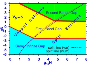
In Fig. 2, the entire family of the symmetric solitons is displayed in the parameter plane of the strength of the in-traspecies and interspecies interactions 共gN,g12N兲. The VA prediction for border between the unsplit and split solitons, given by Eq.共11兲, provides a remarkably accurate fit to the numerical findings.

DependencesN共␮兲for families of symmetric solitons are plotted in Fig.3. It is known that a necessary stability con-dition for solitons populating the semi-infinite gap is given by the Vakhitov-Kolokolov共VK兲criterion, dN/_{d␮⬍0 关16兴,}

0 0.2 0.4 0.6 0.8 1

-3 -2 -1 0 1 2 3

u1,2 2 (x)

x second bandgap

g = 0.003

g12= 0.005

varµ= 1.91

0 0.2 0.4 0.6 0.8 1

-3 -2 -1 0 1 2 3

u1,2 2 (x)

x second bandgap

g = 0.003

g12= 0.005

varµ= 1.91 µ₁= 1.90

0 0.2 0.4 0.6 0.8 1

-3 -2 -1 0 1 2 3

u1,2 2 (x)

x second bandgap

g = 0.003

g12= 0.005

varµ= 1.91 µ₁= 1.90 µ₂= 1.90

0 0.2 0.4 0.6 0.8 1

-3 -2 -1 0 1 2 3

u1,2 2 (x)

x second bandgap

g = 0.003

g12= 0.005

0 0.2 0.4 0.6 0.8 1

-3 -2 -1 0 1 2 3

u1,2 2 (x)

x second bandgap

g = 0.0025

g12= 0.006

µ1= 1.72

0 0.2 0.4 0.6 0.8 1

-3 -2 -1 0 1 2 3

u1,2 2 (x)

x second bandgap

g = 0.0025

g12= 0.006

µ1= 1.72

µ₂= 1.72

0 0.2 0.4 0.6 0.8 1

-3 -2 -1 0 1 2 3

u1,2 2 (x)

x second bandgap

g = 0.0025

g12= 0.006

(a)

(b)

FIG. 1.共Color online兲Examples of unsplit and split symmetric solitons, withN₁=N₂= 1000, trapped in potential −V₀cos共2x兲. Here and in all other figures,V0= 5. For the unsplit soliton, the variational profile is included too.

-6 -5 -4 -3 -2 -1 0 1 2 3 4 5

0 1 2 3 4 5 6 7 8

gN

g₁₂N V₀= 5

-6 -5 -4 -3 -2 -1 0 1 2 3 4 5

0 1 2 3 4 5 6 7 8

gN

g₁₂N V₀= 5

-6 -5 -4 -3 -2 -1 0 1 2 3 4 5

0 1 2 3 4 5 6 7 8

gN

g₁₂N V₀= 5

-6 -5 -4 -3 -2 -1 0 1 2 3 4 5

0 1 2 3 4 5 6 7 8

gN

g₁₂N V₀= 5

-6 -5 -4 -3 -2 -1 0 1 2 3 4 5

0 1 2 3 4 5 6 7 8

gN

g₁₂N V₀= 5

-6 -5 -4 -3 -2 -1 0 1 2 3 4 5

0 1 2 3 4 5 6 7 8

gN

g₁₂N V₀= 5

-6 -5 -4 -3 -2 -1 0 1 2 3 4 5

0 1 2 3 4 5 6 7 8

gN

g₁₂N V₀= 5

-6 -5 -4 -3 -2 -1 0 1 2 3 4 5

0 1 2 3 4 5 6 7 8

gN

g₁₂N V₀= 5

Sp l it

So l it o

ns

Un sp

l it So

l it o ns -6 -5 -4 -3 -2 -1 0 1 2 3 4 5

0 1 2 3 4 5 6 7 8

gN

g₁₂N V₀= 5

Sp l it

So l it o

ns

Un sp

l it So

l it o ns -6 -5 -4 -3 -2 -1 0 1 2 3 4 5

0 1 2 3 4 5 6 7 8

gN

g₁₂N V₀= 5

Sp l it

So l it o

ns

Un sp

l it So

l it o ns -6 -5 -4 -3 -2 -1 0 1 2 3 4 5

0 1 2 3 4 5 6 7 8

gN

g₁₂N V₀= 5

Sp l it

So l it o

ns

Un sp

l it So

l it o ns

split line (var)

-6 -5 -4 -3 -2 -1 0 1 2 3 4 5

0 1 2 3 4 5 6 7 8

gN

g₁₂N V₀= 5

Sp l it

So l it o

ns

Un sp

l it So

l it o ns

split line (var) split line (num)

-6 -5 -4 -3 -2 -1 0 1 2 3 4 5

0 1 2 3 4 5 6 7 8

gN

g₁₂N V₀= 5

Sp l it

So l it o

ns

Un sp

l it So

l it o ns

Second Band Gap

First Band Gap

Semi Infinite Gap

FIG. 2. 共Color online兲 The family of the two-component sym-metric solitons共N₁=N₂⬅N兲, mapped into the plane of the interac-tion strengthsg12NandgN. The plane is divided into regions cor-responding to the semi-infinite gap and the finite first and second band gaps. They are separated by narrow stripes representing the Bloch bands. The border between the unsplit and split solitons is shown as found from the numerical data, and as predicted by Eq. 共11兲.

0 1 2 3 4

-7 -6 -5 -4 -3 -2 -1 0 1 2 3 4

N

/1000

µ

G=10000g

V₀= 5

g₁₂=0.002 G=25 0 1 2 3 4

-7 -6 -5 -4 -3 -2 -1 0 1 2 3 4

N

/1000

µ

G=10000g

V₀= 5

g₁₂=0.002 G=25 G=10 0 1 2 3 4

-7 -6 -5 -4 -3 -2 -1 0 1 2 3 4

N

/1000

µ

G=10000g

V₀= 5

g₁₂=0.002 G=25 G=10 G=0 0 1 2 3 4

-7 -6 -5 -4 -3 -2 -1 0 1 2 3 4

N

/1000

µ

G=10000g

V₀= 5

g₁₂=0.002 G=25 G=10 G=0 G=-5 0 1 2 3 4

-7 -6 -5 -4 -3 -2 -1 0 1 2 3 4

N

/1000

µ

G=10000g

V₀= 5

g₁₂=0.002 G=25 G=10 G=0 G=-5 G=-10 0 1 2 3 4

-7 -6 -5 -4 -3 -2 -1 0 1 2 3 4

N

/1000

µ

G=10000g

V₀= 5

g₁₂=0.002 G=25 G=10 G=0 G=-5 G=-10 G=-25 0 1 2 3 4

-7 -6 -5 -4 -3 -2 -1 0 1 2 3 4

N

/1000

µ

G=10000g

V₀= 5

g₁₂=0.002

0 1 2 3 4

-7 -6 -5 -4 -3 -2 -1 0 1 2 3 4

N

/1000

µ

G=10000g

V₀= 5

g₁₂=0.002

0 1 2 3 4

-7 -6 -5 -4 -3 -2 -1 0 1 2 3 4

N

/1000

µ

G=10000g

V₀= 5

g₁₂=0.002

while stable solitons in finite band gaps have dN/d␮⬎0, disobeying this criterion 关3,15兴. In the present case, Fig. 3 shows the same generic feature共the semi-infinite gap con-tains solitons only for g⬍0, i.e., in the case of the self-attraction兲. A noteworthy feature, viz, a turning point in de-pendenceN共␮兲, is exhibited for g= −0.001 by the solution branch which passes from the semi-infinite gap into the first finite band gap, and also by the branch corresponding to g = −0.0005. Consequently, two differentstablesolitons can be found in the corresponding interval of ␮. The solitons be-longing to the branches withg= 0.0025, g= 0.001, andg= 0 in Fig.3are unsplit, and they are accurately predicted by the VA. Accordingly, the curves for these branches, as obtained from the VA and from the numerical data, are virtually iden-tical. On the other hand, all solitons belonging to the branch withg= −0.0025 exhibit splitting. As concerns the bending branches, their parts below the turning point are formed by unsplit solitons共which are accurately approximated by the VA兲, while above the turning point the family continues in the split form. Accordingly, the turning point on each bend-ing branch belongs to the splittbend-ing border for the symmetric solitons, cf. Fig.2.

Asymmetric solitons. Typical examples of solitons with N1⫽N2 are displayed in Fig. 4. Similar to their symmetric counterparts, cf. Fig. 1, they feature both unsplit and split shapes共the former ones are well approximated by the VA兲, which are again confined to a single cell of the OL potential.

0 1 2 3 4 5

0 1 2 3 4 5

N2

/1000

N₁/1000

g = 0.001 g₁₂ = 0.002

first gap second gap inter gap (1-2) inter gap (1-2) 0 1 2 3 4 5

0 1 2 3 4 5

N2

/1000

N₁/1000

g = 0.001 g₁₂ = 0.002

first gap second gap inter gap (1-2) inter gap (1-2) 0 1 2 3 4 5

0 1 2 3 4 5

N2

/1000

N₁/1000

g = 0.001 g₁₂ = 0.002

first gap second gap inter gap (1-2) inter gap (1-2) 0 1 2 3 4 5

0 1 2 3 4 5

N2

/1000

N₁/1000

g = 0.001 g₁₂ = 0.002

first gap second gap inter gap (1-2) inter gap (1-2) 0 1 2 3 4 5

0 1 2 3 4 5

N2

/1000

N₁/1000

g = 0.001 g₁₂ = 0.002

first gap second gap inter gap (1-2) inter gap (1-2) 0 1 2 3 4 5

0 1 2 3 4 5

N2

/1000

N₁/1000

g = 0.001 g₁₂ = 0.002

first gap second gap inter gap (1-2) inter gap (1-2) 0 1 2 3 4 5

0 1 2 3 4 5

N2

/1000

N₁/1000

g = 0.001 g₁₂ = 0.002

first gap second gap inter gap (1-2) inter gap (1-2) 0 1 2 3 4 5

0 1 2 3 4 5

N2

/1000

N₁/1000

g = 0.001 g₁₂ = 0.002

first gap second gap inter gap (1-2) inter gap (1-2) 0 1 2 3 4 5

0 1 2 3 4 5

N2

/1000

N₁/1000

g = 0.001 g₁₂ = 0.002

first gap second gap inter gap (1-2) inter gap (1-2) 0 1 2 3 4 5

0 1 2 3 4 5

N2

/1000

N₁/1000

g = 0.001 g₁₂ = 0.002

first gap second gap inter gap (1-2) inter gap (1-2) border (var) 0 1 2 3 4 5

0 1 2 3 4 5

N2

/1000

N₁/1000

g = 0.001 g₁₂ = 0.002

first gap second gap inter gap (1-2) inter gap (1-2) border (var) split line 0 1 2 3 4 5 6 7

0 1 2 3 4 5 6 7

N2

/1000

N₁/1000 g = -0.001 g₁₂ = 0.002

first gap semi infinite gap inter gap (0-1) inter gap (0-1) inter gap (0-2)

inter gap(0-2)

0 1 2 3 4 5 6 7

0 1 2 3 4 5 6 7

N2

/1000

N₁/1000 g = -0.001 g₁₂ = 0.002

first gap semi infinite gap inter gap (0-1) inter gap (0-1) inter gap (0-2)

inter gap(0-2)

0 1 2 3 4 5 6 7

0 1 2 3 4 5 6 7

N2

/1000

N₁/1000 g = -0.001 g₁₂ = 0.002

first gap semi infinite gap inter gap (0-1) inter gap (0-1) inter gap (0-2)

inter gap(0-2)

0 1 2 3 4 5 6 7

0 1 2 3 4 5 6 7

N2

/1000

N₁/1000 g = -0.001 g₁₂ = 0.002

first gap semi infinite gap inter gap (0-1) inter gap (0-1) inter gap (0-2)

inter gap(0-2)

0 1 2 3 4 5 6 7

0 1 2 3 4 5 6 7

N2

/1000

N₁/1000 g = -0.001 g₁₂ = 0.002

first gap semi infinite gap inter gap (0-1) inter gap (0-1) inter gap (0-2)

inter gap(0-2)

0 1 2 3 4 5 6 7

0 1 2 3 4 5 6 7

N2

/1000

N₁/1000 g = -0.001 g₁₂ = 0.002

first gap semi infinite gap inter gap (0-1) inter gap (0-1) inter gap (0-2)

inter gap(0-2)

0 1 2 3 4 5 6 7

0 1 2 3 4 5 6 7

N2

/1000

N₁/1000 g = -0.001 g₁₂ = 0.002

first gap semi infinite gap inter gap (0-1) inter gap (0-1) inter gap (0-2)

inter gap(0-2)

0 1 2 3 4 5 6 7

0 1 2 3 4 5 6 7

N2

/1000

N₁/1000 g = -0.001 g₁₂ = 0.002

first gap semi infinite gap inter gap (0-1) inter gap (0-1) inter gap (0-2)

inter gap(0-2)

split line 0 1 2 3 4 5 6 7

0 1 2 3 4 5 6 7

N2

/1000

N₁/1000 g = -0.001 g₁₂ = 0.002

first gap semi infinite gap inter gap (0-1) inter gap (0-1) inter gap (0-2)

inter gap(0-2)

split line border (var) 0 1 2 3 4 5 6 7

0 1 2 3 4 5 6 7

N2

/1000

N₁/1000 g = -0.001 g₁₂ = 0.002

first gap semi infinite gap inter gap (0-1) inter gap (0-1) inter gap (0-2)

inter gap(0-2)

0 1 2 3 4 5 6 7

0 1 2 3 4 5 6 7

N2

/1000

N₁/1000 g = -0.001 g₁₂ = 0.002

first gap semi infinite gap inter gap (0-1) inter gap (0-1) inter gap (0-2)

inter gap(0-2)

0 1 2 3 4 5 6 7

0 1 2 3 4 5 6 7

N2

/1000

N₁/1000 g = -0.001 g₁₂ = 0.002

first gap semi infinite gap inter gap (0-1) inter gap (0-1) inter gap (0-2)

inter gap(0-2)

0 1 2 3 4 5 6 7

0 1 2 3 4 5 6 7

N2

/1000

N₁/1000 g = -0.001 g₁₂ = 0.002

first gap semi infinite gap inter gap (0-1) inter gap (0-1) inter gap (0-2)

inter gap(0-2)

0 1 2 3 4 5 6 7

0 1 2 3 4 5 6 7

N2

/1000

N₁/1000 g = -0.001 g₁₂ = 0.002

first gap semi infinite gap inter gap (0-1) inter gap (0-1) inter gap (0-2)

inter gap(0-2)

0 1 2 3 4 5 6

0 1 2 3 4 5 6

N2

/1000

N₁/1000 g = 0

g₁₂ = 0.002

first gap inter gap(1-2) inter gap (1-2) 0 1 2 3 4 5 6

0 1 2 3 4 5 6

N2

/1000

N₁/1000 g = 0

g₁₂ = 0.002

first gap inter gap(1-2) inter gap (1-2) 0 1 2 3 4 5 6

0 1 2 3 4 5 6

N2

/1000

N₁/1000 g = 0

g₁₂ = 0.002

first gap inter gap(1-2) inter gap (1-2) 0 1 2 3 4 5 6

0 1 2 3 4 5 6

N2

/1000

N₁/1000 g = 0

g₁₂ = 0.002

first gap inter gap(1-2) inter gap (1-2) 0 1 2 3 4 5 6

0 1 2 3 4 5 6

N2

/1000

N₁/1000 g = 0

g₁₂ = 0.002

first gap inter gap(1-2) inter gap (1-2) 0 1 2 3 4 5 6

0 1 2 3 4 5 6

N2

/1000

N₁/1000 g = 0

g₁₂ = 0.002

first gap inter gap(1-2) inter gap (1-2) split line 0 1 2 3 4 5 6

0 1 2 3 4 5 6

N2

/1000

N₁/1000 g = 0

g₁₂ = 0.002

first gap inter gap(1-2) inter gap (1-2) split line border (var) (c) (b) (a)

FIG. 5. 共Color online兲Families of asymmetric and symmetric solitons mapped into the plane of atom numbers N1 and N2, for differentg12andg. The plane is divided into regions populated by solitons of six different types 共three intragap and three intergap varieties, symbols 0 and 1, 2 standing for the semi-infinite and two lowest finite band gaps, respectively兲. Each panel also shows the numerically found border between the unsplit and split solitons, and borders between different types of the unsplit ones, as predicted by the VA.

0 0.4 0.8 1.2

-3 -2 -1 0 1 2 3

u

2 1,2

(x)

x first-second

N₁= 500 N₂= 4000 g = 0.002 g₁₂= 0.0005

varµ₁= -0.93

0 0.4 0.8 1.2

-3 -2 -1 0 1 2 3

u

2 1,2

(x)

x first-second

N₁= 500 N₂= 4000 g = 0.002 g₁₂= 0.0005

varµ₁= -0.93

varµ₂= 2.03

0 0.4 0.8 1.2

-3 -2 -1 0 1 2 3

u

2 1,2

(x)

x first-second

N₁= 500 N₂= 4000 g = 0.002 g₁₂= 0.0005

varµ₁= -0.93

varµ₂= 2.03 µ₁= -0.93

0 0.4 0.8 1.2

-3 -2 -1 0 1 2 3

u

2 1,2

(x)

x first-second

N₁= 500 N₂= 4000 g = 0.002 g₁₂= 0.0005

varµ₁= -0.93

varµ₂= 2.03 µ₁= -0.93 µ₂= 2.04

0 0.4 0.8 1.2

-3 -2 -1 0 1 2 3

u

2 1,2

(x)

x first-second

N₁= 500 N₂= 4000 g = 0.002 g₁₂= 0.0005

0 0.6 1.2 1.8

-3 -2 -1 0 1 2 3

u

2 1,2

(x)

x second-semi-infinite N₁= 500

N₂= 2000 g = -0.002 g₁₂= 0.0065

µ₁= 1.70

0 0.6 1.2 1.8

-3 -2 -1 0 1 2 3

u

2 1,2

(x)

x second-semi-infinite N₁= 500

N₂= 2000 g = -0.002 g₁₂= 0.0065

µ₁= 1.70 µ₂= -6.60

0 0.6 1.2 1.8

-3 -2 -1 0 1 2 3

u

2 1,2

(x)

x second-semi-infinite N₁= 500

N₂= 2000 g = -0.002 g₁₂= 0.0065

(a)

(b)

The entire family of asymmetric and symmetric GSs is mapped in the共N1,N2兲plane, at fixed values of the interac-tion coefficients共g12andg兲in Fig.5. In these diagrams, the border between intragap solitons of different types shrink to a point belonging to the diagonal line共N1=N2兲, which cor-responds to symmetric solitons that account for direct tran-sitions between different types of intragap solitons. In Fig.5 the VA for the unsplit solitons accurately predicts borders between their different varieties.

If none of the nonlinearities is attractive 关Figs.5共a兲 and 5共b兲兴, no chemical potential may fall in the semi-infinite gap. Three types of GSs are possible if both nonlinearities are repulsive 关Fig. 5共a兲兴: intragap ones, in the two finite band gaps, and the intergap species, combining them. If the in-traspecies nonlinearity exactly vanishes关Fig.5共b兲兴, the inter-species repulsion cannot push both components into the sec-ond finite band gap, which leaves us with two species: intragap in the first band gap, and the one mixing the two finite band gaps. The interplay of the attractive intraspecies nonlinearity with the interspecies repulsion supports two in-tragap and two intergap types, as seen in Fig.5共c兲. Note that one of them skips the first band gap, binding together com-ponents sitting in the semi-infinite and in second finite gaps. A notable feature of the map in Fig.5共c兲is the smooth tran-sition from ordinary solitons, with both components in the semi-infinite gap, to ones of the semigap type.

IV. CONCLUSION

In this work, we have considered the interplay of the re-pulsion between two species of bosonic atoms with

intraspe-cies repulsion or attraction in a binary BEC mixture loaded into the OL potential. Families of stable solitons found in this setting are classified as symmetric or asymmetric, split or unsplit, and intragap or intergap. Three varieties of intragap solitons, and another three types of intergap ones are identi-fied, if the consideration is limited to the two lowest finite band gaps of the OL-induced spectrum. Varying the atom numbers in the two componentsN1,2, we have plotted maps of various states. Although different intragap and intergap species are separated by Bloch bands, transitions between them are continuous in the 共N₁,N₂兲 plane. In particular, a solution branch which connects the solitons 共of the split type兲, populating the semi-infinite gap, and unsplit solitons in the first finite band gap, features the turning point at the border between the two varieties. Other varieties revealed by the analysis represent semigap solitons, with one component belonging to the semi-infinite gap, and the other one falling into a finite band gap.

A considerable part of the numerical findings reported in this work was accurately predicted by variational approxima-tion. These include the shape of unsplit solitons共both sym-metric and asymsym-metric ones兲, borders between their variet-ies, and the splitting border for the symmetric solitons.

ACKNOWLEDGMENTS

We appreciate support from FAPESP and CNPq共Brazil兲, and Israel Science Foundation 共Center of Excellence Grant No. 8006/03兲.

关1兴V. M. Pérez-García, H. Michinel, and H. Herrero, Phys. Rev. A 57, 3837共1998兲; F. Kh. Abdullaevet al., Int. J. Mod. Phys. B 19, 3415共2005兲.

关2兴K. E. Streckeret al., Nature 共London兲 417, 150 共2002兲; L. Khaykovichet al., Science256, 1290共2002兲; S. L. Cornish, S. T. Thompson, and C. E. Wieman, Phys. Rev. Lett. 96, 170401 共2006兲.

关3兴O. Zobay, S. Potting, P. Meystre, and E. M. Wright, Phys. Rev. A 59, 643共1999兲; A. Trombettoni and A. Smerzi, Phys. Rev. Lett. 86, 2353共2001兲; B. B. Baizakov, V. V. Konotop, and M. Salerno, J. Phys. B 35, 51015 共2002兲; P. J. Y. Louis, E. A. Ostrovskaya, C. M. Savage, and Y. S. Kivshar, Phys. Rev. A

67, 013602共2003兲.

关4兴K. M. Hilligsøe, M. K. Oberthaler, and K.-P. Marzlin, Phys. Rev. A 66, 063605 共2002兲; D. E. Pelinovsky, A. A. Sukho-rukov, and Y. S. Kivshar, Phys. Rev. E 70, 036618共2004兲. 关5兴B. Eiermann, T. Anker, M. Albiez, M. Taglieber, P. Treutlein,

K. P. Marzlin, and M. K. Oberthaler, Phys. Rev. Lett. 92, 230401 共2004兲; O. Morsch and M. Oberthaler, Rev. Mod. Phys. 78, 179共2006兲.

关6兴V. Ahufinger, A. Sanpera, P. Pedri, L. Santos, and M. Lewen-stein, Phys. Rev. A 69, 053604共2004兲.

关7兴M. Matuszewski, W. Krolikowski, M. Trippenbach, and Y. S. Kivshar, Phys. Rev. A 73, 063621共2006兲.

关8兴C. J. Myatt, E. A. Burt, R. W. Ghrist, E. A. Cornell, and C. E. Wieman, Phys. Rev. Lett. 78, 586 共1997兲; D. M. Stamper-Kurn, M. R. Andrews, A. P. Chikkatur, S. Inouye, H. J. Miesner, J. Stenger, and W. Ketterle,ibid. 80, 2027共1998兲. 关9兴A. Simoni, F. Ferlaino, G. Roati, G. Modugno, and M.

Ingus-cio, Phys. Rev. Lett. 90, 163202共2003兲.

关10兴V. M. Pérez-García and J. B. Beitia, Phys. Rev. A 72, 033620 共2005兲; S. K. Adhikari, Phys. Lett. A 346, 179共2005兲; Phys. Rev. A 72, 053608共2005兲; J. Phys. A 40, 2673共2007兲. 关11兴A. Gubeskys, B. A. Malomed, and I. M. Merhasin, Phys. Rev.

A 73, 023607共2006兲.

关12兴M. Matuszewski, B. A. Malomed, and M. Trippenbach, Phys. Rev. A 76, 043826共2007兲.

关13兴V. M. Pérez-García, H. Michinel, J. I. Cirac, M. Lewenstein, and P. Zoller, Phys. Rev. A 56, 1424共1997兲.

关14兴L. Salasnich, A. Parola, and L. Reatto, Phys. Rev. A 65, 043614 共2002兲; L. Salasnich and B. A. Malomed, ibid. 74, 053610共2006兲.

关15兴S. K. Adhikari and B. A. Malomed, Europhys. Lett. 79, 50003 共2007兲; Phys. Rev. A 76, 043626共2007兲.