INSTITUTO DE INVESTIGAÇÃO E FORMAÇÃO AVANÇADA ÉVORA, 2015 ORIENTADORES:Prof.ª Dr.ª Maria Madalena Vitório Moreira Vasconcelos Prof. Dr. João Alexandre Medina Corte-Real
Tese apresentada à Universidade de Évora
para obtenção do Grau de Doutor em
Ciências da Engenharia do Território e Ambiente
Especialidade:
Engenharia Civil
Rong Zhang
INTEGRATED MODELLING FOR
EVALUATION OF CLIMATE CHANGE
IMPACTS ON AGRICULTURAL
DOMINATED BASIN
Tese de Doutoramento financiada pelo Ministério da Educação e Ciência Fundação para a Ciência e a Tecnologia
Bolsa de Doutoramento SFRH/BD/48820/2008
致我父亲和母亲:感谢您们让我的梦想变成了现实 致我叔叔和婶婶:感谢您们永无止境的支持和鼓励 To Professors Cui GuangBai and João Corte-Real: Thank you for having opened a door to a wonderful world Ao meu amor Sandro: Obrigada por fazer parte da minha vida
Acknowledgments
I would like to thank my supervisors, Prof. Madalena Moreira and Prof. João Corte-Real, for their invaluable guidance and support throughout the period of this research. This thesis was made possible by a PhD grant of Portuguese national funding agency for science, research and technology (SFRH/BD/48820/2008). I am very grateful to Prof. Francisco Sepúlveda Texeira, vice-president of FCT in 2008, and Mrs. Gertrudes Almeida for the opportunity of fellowship.
I wish to thank the support from the projects ERLAND (PTDC/AAC-AMB/100520/2008), CLIPE (PTDC/AAC-CLI/111733/2009) and KLIMHIST (PTDC/AAC-CLI/119078/2010), the observed data from SNIRH, SAGRA/COTR and IPMA and the climate model data provided by the EU-FP6 project ENSEMBLES.
I am deeply grateful to Prof. Cui Guangbai, my previous supervisor in Hohai University, China, for his great advice, encouragement and support to the opportunity of this research.
I very much appreciate the twice opportunities offered by Prof. Chris Kilsby for me to visit Newcastle University to have training courses on SHETRAN model and development of weather generator applications. I would like to thank him and his colleagues, Dr. James Bathurst, Prof. John Ewen, Dr. Stephen Birkinshaw, Dr. Isabella Bovolo, Prof. Hayley Fowler, Dr. Aidan Burton, Dr. Stephen Blenkinsop, Dr. Greg O’Donnell and Dr. Nathan Forsythe, for the observed data, great assistance and helpful discussions.
I would like to thank Prof. Celso Santos and Dr. Paula Freire for their valuable visit to University of Évora. The collaboration was very helpful and fruitful.
I would further like to thank Prof. Ricardo Serralheiro, Prof. Lúcio Santos, Prof. Elsa Sampaio, Prof. Shakib Shahidian, Dr. Qian Budong, Dr. Sandra Mourato, Dr. Célia Toureiro and Dr. Júlio Lima for help, comments and scientific discussions during the elaboration of this thesis.
I would like to thank my friends at University of Évora, Hohai University and Newcastle University for making my stay so enjoyable. Special Thanks go to Prof. José Peça, Regina Corte-Real, Isilda Menezes, Susana Mendes, Luiz Tadeu Silva, Cláudia Vicente, Clarisse Brígido, Guilhermina Pias, Maria João Vila Viçosa, Ana Canas, Lígia Justo, Elisete Macedo, Véronica Moreno, Cláudia Furtado, Marco Machado, Amaia Nogales, Daniel Malet and Lemos Djata.
I want to thank my family for all their love and support. I would like to thank Sandro Veiga and his family for all the encouragement and support.
i
Integrated Modelling for Evaluation of Climate
Change Impacts on Agricultural Dominated
Basin
Abstract
This study evaluated future climate change impacts on water resources, extreme discharges and sediment yields for the medium-sized (705-km2) agriculture dominated Cobres basin, Portugal, in the context of anti-desertification strategies. We applied the physically-based spatially-distributed hydrological model—SHETRAN, obtaining the optimized parameters and spatial resolution by using the Modified Shuffled Complex Evolution (MSCE) method and the Non-dominated Sorting Genetic Algorithm II (NSGA-II), to simulate the hydrological processes of runoff and sediment transport. We used the model RanSim V3, the rainfall conditioned weather generator—ICAAM-WG, developed in this study, based on the modified Climate Research Unit daily Weather Generator (CRU-WG), and SHETRAN, to downscale projections of change for 2041– 2070, from the RCM HadRM3Q0 with boundary conditions provided by the AOGCM HadCM3Q0, provided by the ENSEMBLES project, under SRES A1B emission scenario.
We found future climate with increased meteorological, agricultural and hydrological droughts. The future mean annual rainfall, actual evapotranspiration, runoff and sediment yield are projected to decrease by the orders of magnitude of respectively ~88 mm (19%), ~41 mm (11%), ~48 mm (50%) and ~1.06 t/ha/year (45%). We also found reductions in extreme runoff and sediment discharges, for return periods smaller than 20 years; however for return periods in the range of 20–50 years, future extremes are of the same order of magnitude of those in the reference climate.
iii
Modelação integrada para avaliação dos
impactos das alterações climáticas sobre
bacias
hidrográficas
com
uso
predominantemente agrícola
Resumo
Neste estudo são avaliados os impactos futuros das alterações climáticas nos recursos hídricos e em extremos do escoamento e transporte de sedimentos, na bacia hidrográfica do rio Cobres, Portugal, agrícola, de dimensão média (705 Km2), no contexto do combate à desertificação. Foi aplicado o modelo hidrológico fisicamente baseado e espacialmente distribuído SHETRAN, tendo sido obtidos os valores optimizados de parâmetros e da resolução espacial, utilizando o método “Modified Shuffled Complex Evolution” (MSCE) e o algoritmo “Non-dominated Sorting Genetic Algorithm II” (NSGA-II), para simular os processos hidrológicos de escoamento e transportes de sedimentos. Foram utilizados o modelo de RainSim V3, o gerador de tempo ICAAM-WG, desenvolvido neste estudo, baseado no CRU-WG, e o SHETRAN, para o “downscaling” das projecções climáticas para 2041 – 2070, geradas pelo MRC HadRM3Q0 com condições de fronteira fornecida pelo MCG HadCM3Q0, projecto ENSEMBLES, sob o cenário SRES A1B.
O clima futuro é caracterizado por um número crescente de secas meteorológicas, agrícolas e hidrológicas. Os valores médios anuais da precipitação, evapotranspiração real, escoamento superficial e transporte de sedimentos, revelam decréscimos com ordens de grandeza respectivamente de ~88 mm (19%), ~41 mm (11%), ~48 mm (50%) e ~1.06 t/há/ano (45%). Encontraram-se ainda reduções nos valores extremos do escoamento superficial e do transporte de sedimentos para períodos de retorno inferiores a 20 anos; contudo, para períodos de retorno no intervalo 20–50 anos, os valores extremos futuros apresentam a mesma ordem de grandeza que os relativos ao período de referência mas mantendo níveis equivalentes para os com 20–50 anos.
v
气候变化对农业为主流域的影响的综合模拟
摘要
水资源短缺和沙漠化是葡萄牙南部地区面临的主要问题。为了给沙漠化防治对策提供科 学依据,本文评估了气候变化对葡萄牙南部以农业为主的科布热斯流域(Cobres,面积约 705 km2 )的水资源、暴雨径流和泥沙流失的影响。采用基于物理机制的分布式水文模型 SHETRAN 模拟径流和泥沙迁移的水文过程,并运用 MSCE(Modified Shuffled Complex Evolution)方法和 NSGA-II(Non-dominated Sorting Genetic Algorithm II)算法优化 模型参数和空间步长.采用奈曼–斯科特时空矩形脉冲(STNSRP)模型 RainSimV3,本研 究开发的基于改进的英国气候研究所(Climate Research Unit)天气发生器(CRU-WG)的 雨控天气发生器 ICAAM-WG,对由 ENSEMBLES 项目提供的基于 SRES A1B 温室气体排放情 景下由全球气候模式 HadCM3Q0 提供边界条件的区域气候模式 HadRM3Q0 所模拟的 2041-2070 年间的气候变化情景做降尺度分析。结果表明,未来该地区的气象干旱、农业干旱 和水文干旱都有加重趋势。未来平均年降雨、蒸散发量、径流和产沙量预计将比现在分 别减少数量级约 88 毫米(19%)、41 毫米(11%)、48 毫米(50%)和 1.06 吨/公顷/年 (45%)。并且,我们预计重现期在 20 年以下的极端径流和输沙量都将减少,重现期在 20–50 年范围内极端径流和输沙量将保持与基准气候模式相同数量级。vii
Index
Abstract ... i Resumo ... iii 摘要 ... v List of Figures ... xiList of Tables... xix
List of Symbols and Abbreviations ... xxi
1. Introduction and Objectives ... 1
2. Scientific Background ... 3
2.1 Problems of Southern Portugal... 3
2.2 Hydrological Impacts Assessments ... 4
2.3 Problems Involved in the Use of Physically-Based Spatially-Distributed Hydrological Models ... 6
3. Cobres Basin ... 9
3.1 Geographical and Climatological Context ... 9
3.2 Hydrological Data ... 10
3.3 Sediment Data ... 12
4. SHETRAN Modelling System ... 15
4.1 Water Flow Component ... 15
4.1.1 Interception and Evapotranspiration Module ... 15
4.1.2 Overland and Channel Flow Module ... 16
4.1.3 Variably Saturated Subsurface Module... 17
4.2 Sediment Transport Component ... 18
4.2.1 Hillslope Sediment Transport Module ... 18
4.2.2 Channel Sediment Transport Module ... 20
5. Calibration of SHETRAN Model ... 23
viii
5.2 Calibration Parameters ... 25
5.3 SHETRAN Model Set-Up... 25
5.4 The Objective Function ... 29
5.5 Automatic Calibration of SHETRAN Model by MSCE ... 32
5.5.1 The MSCE Optimization Algorithm ... 32
5.5.2 MSCE Calibration of SHETRAN Hydrological Parameters ... 33
5.6 Multi-Objective Calibration of SHETRAN Model by NSGA-II ... 42
5.6.1 The NSGA-II Optimization Algorithm ... 42
5.6.2 Performance Metrics of NSGA-II Algorithm ... 44
5.6.3 NSGA-II Calibration of SHETRAN Hydrological Parameters ... 45
5.6.4 NSGA-II Calibration of SHETRAN Sediment Parameters... 53
5.7 Discussion ... 60
6. Impacts of Spatial Scale on the SHETRAN Model ... 63
6.1 Introduction ... 63
6.2 Methods and Data ... 64
6.3 Impacts of Spatial Scale on the SHETRAN Model Input ... 66
6.4 Impacts of Spatial Scale on the SHETRAN Model Performance ... 70
6.4.1 Introduction ... 70
6.4.2 Impacts of Spatial Scale on Long-Term Runoff Simulation ... 70
6.4.3 Impacts of Spatial Scale on Storm-Runoff Generation ... 84
6.5 Discussion ... 89
7. Downscaling of Climate Change Scenarios ... 91
7.1 Introduction ... 91
7.2 Methodology and Data ... 93
7.2.1 Data Preparation ... 93
7.2.2 Multi-Site Daily Precipitation Time Series: the RainSim V3 Model ... 98
7.2.3 Daily Temperature and Evapotranspiration Time Series: the Weather Generator (ICAAM-WG) Model ... 99
7.2.4 Change Factors Calculation for Future Time Slice 2041–2070 ... 101
7.2.5 Outline of the Climate Downscaling Method ... 104
7.3 Results of Control Climate Simulations ... 104
7.3.1 Validation of the RainSim V3 Model ... 104
ix
7.4 Results of Future Climate Simulations ... 111
7.4.1 Simulation of Future Precipitation ... 111
7.4.2 Simulation of Future PET ... 121
7.5 Discussion ... 122
8. Assessment of Future Climate Change Impacts ... 125
8.1 Introduction ... 125
8.2 Methodology ... 126
8.2.1 SHETRAN Model Simulation ... 126
8.2.2 Statistical Methods ... 127
8.3 Assessment of Future Climate Change Impacts... 129
8.3.1 Future Climate Change Impacts on Water Availability and Sediment Yield 130 8.3.2 Future Climate Change Impacts on Extreme Events ... 135
8.4 Discussion ... 141
9. Conclusions and Expectations ... 145
9.1 Summary ... 145
9.2 Main Achievements ... 146
9.3 Main Limitations of the Work ... 147
9.4 Further Research ... 147
10. References ... 149
Appendices ... 163
Appendix 1: Sensitivity Analysis for the SHETRAN Simulation at Cobres Basin with Spatial Resolution of 2.0 Km and Temporal Resolution of 1.0 Km ... 163
Appendix 2: The Proposed Autoregressive Processes in the ICAAM-WG Model ... 166
Appendix 3: Schematic Summary of the Procedure to Downscale the Climate Change Scenarios. ... 167
Appendix 4: Plots for Control and Future Rainfall Simulations ... 171
Appendix 5: Frequency Distribution of GEV, Gamma and Three-Parameter Lognormal Distributions ... 175
A5.1 GEV Distribution: ... 175
A5.2 Gamma Distribution: ... 175
xi
List of Figures
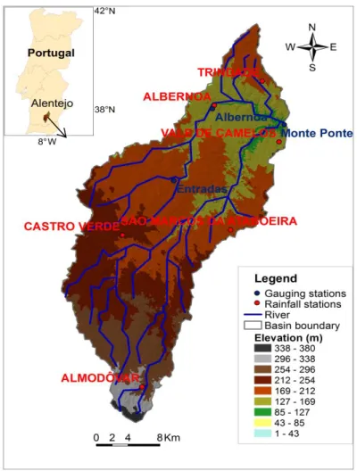
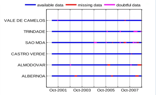
Fig. 3.1 Map showing elevations, gauging stations, rainfall stations and watercourses of the Cobres basin. ... 9 Fig. 3.2 Data availability analysis for hourly rainfall series at stations in the Cobres basin (SAO MDA denotes the São Marcos da Ataboeira station). ... 11 Fig. 3.3 Double mass curve for monthly rainfall of 6 stations from January 2001 to September 2009. ... 11 Fig. 3.4 Plot for comparison between linear and quadratic regressions. ... 14 Fig. 5.1 Location map, SHETRAN grid network (abscissa and ordinate indicate grid cell number) and channel system (the heavy blue lines, representing all channel links, and the light blue lines, representing the links used to extract simulated discharges at basin outlet and internal gauging stations) for the Cobres basin, showing the rain gauges (the
red circles) and gauging stations (the blue circles at outlet, northern and central parts of
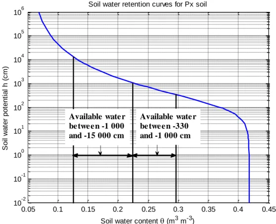
the basin, are respectively Monte da Ponte, Albernoa and Entradas gauging stations). The grid squares have dimensions 2 × 2.0 km2. ... 26 Fig. 5.2 Soil water retention curve for Px soil in Cobres basin (result from MSCE
calibration scenario IV). ... 35 Fig. 5.3 Comparison of observed and simulated discharges from MSCE calibration scenario IV for the Cobres basin with spatial resolution of 2.0 km grid and temporal resolution of 1.0 hour, for main periods of (a) calibration and (b) validation processes.38 Fig. 5.4 Water balance analysis of MSCE calibration scenario IV for calibration and validation periods; P –precipitation, AET – actual evapotranspiration, ΔS – change of subsurface water storage, R – total runoff. ... 39 Fig. 5.5 Comparison of observed and simulated discharges from MSCE calibration scenario IV for the Cobres basin with spatial resolution of 2.0 km grid and temporal resolution of 1.0 hour: (a) Storm No.1 at basin outlet; (b) Storm No.4 at basin outlet; (c) Storm No.4 at internal gauging station Albernoa; (d) Storm No.4 at internal gauging station Entradas. ... 40 Fig. 5.6 (a) The ensemble of approximation sets obtained from the last generation of the 90 trial runs of NSGA-II algorithm for SHETRAN calibration where RMSE, LOGE and NSE are respectively root mean square errors, log-transformed errors and Nash-Sutcliffe Efficiency. The asterisks in red, blue and light blue colors respectively represent (ηc, ηm) with values (0.5, 0.5), (2.0, 0.5) and (20., 20.). Two-dimensional
presentations of figure (a) are shown in (b), (c) and (d). ... 46 Fig. 5.7 (a) The best known approximation sets derived from 30 trial runs of NSGA-II algorithm with (ηc, ηm) of (0.5, 0.5), (2.0, 0.5) and (20., 20.) are respectively shown in
small black squares, filled blue circles and filled purplish red circles. The final one derived from all trial runs is shown in filled red circles. (b) The final best known approximation set is made up of solutions from trial runs of NSGA-II algorithm with (ηc,
ηm) of (0.5, 0.5) and (2.0, 0.5), respectively showing in filled red and blue circles. The
false front, in small black squares, is an example of the approximation set derived from a trapped trial run of the NSGA-II algorithm. ... 47
xii
Fig. 5.8 Plots of dynamic performance results of NSGA-II algorithm, namely hypervolume (a, b and c), Ԑ-indicator (d, e and f), generational distance (g, h and i) and opt-indicator (j, k and l), versus total number of SHETRAN model runs. Mean performance is indicated by a solid line, the standard deviation by a dashed line, and the range of performance by the shaded region. The left, middle and right columns of plots were respectively generated from 30 trial runs of NSGA-II with (ηc, ηm) of (0.5,
0.5), (2.0, 0.5) and (20., 20.). ... 48 Fig. 5.9 Plots of dynamic performance results of NSGA-II algorithm, namely hypervolume (a), Ԑ-indicator (b), generational distance (c) and opt-indicator (d), versus total number of SHETRAN evaluations. The 50th and 95th percentiles of performance are respectively indicated in dash and bold solid lines. The red, blue and light blue lines were respectively generated from 30 trial runs of NSGA-II with (ηc, ηm) of (0.5, 0.5), (2.0,
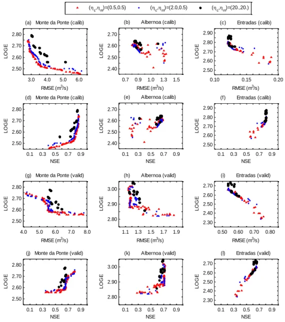
0.5) and (20., 20.). ... 49 Fig. 5.10 Plots of SHETRAN model performance indicators, namely RMSE, LOGE and NSE, at basin outlet Monte da Ponte (a, d, g and j) and internal gauging stations Albernoa (b, e, h and k) and Entradas (c, f, i and l). The results for the calibration period are denoted by “(calib)” and those for the validation period by “(valid)”. The filled red triangles, blue squares and black circles respectively represent the solutions of best known approximation sets derived from 30 trial runs of NSGA-II with (ηc, ηm) of
(0.5, 0.5), (2.0, 0.5) and (20., 20.). ... 50 Fig. 5.11 Comparison between observed and simulated discharges from solutions obtained from automatic calibration of SHETRAN model by NSGA-II algorithm: (a) Storm No.1 at basin outlet; (b) Storm No.4 at basin outlet; (c) Storm No.4 at internal gauging station Albernoa; (d) Storm No.4 at internal gauging station Entradas. “Qsim1”,
“Qsim2”, “Qsim3” and “Qsim4” are SHETRAN simulations, for the calibration period
(2004-2006), with objective functions (RMSE, LOGE, NSE) at basin outlet of respective values (2.81, 2.74, 0.87), (3.81, 2.53, 0.77), (4.85, 2.49, 0.63) and (5.85, 2.46, 0.46). 52 Fig. 5.12 Comparisons between observed and simulated hourly discharges and sediment discharges for the solution obtained from automatic calibration of sediment parameters by NSGA-II. “Qobs”, “Qsim”, “Qsedobs” and “Qsedsim” respectively represent
observed discharge, simulated discharge, observed sediment discharge and simulated sediment discharge. Time is shown in the “MM/DD/YY” format. ... 60 Fig. 6.1 Maps of land-use distribution for Cobres basin with respective spatial resolutions of 0.5, 1.0, 1.5 and 2.0 km. ... 67 Fig. 6.2 Maps of soil type distribution for Cobres basin with respective spatial resolutions of 0.5, 1.0, 1.5 and 2.0 km. ... 68 Fig. 6.3 Maps of river links distribution for Cobres basin with respective spatial resolutions of 0.5, 1.0, 1.5 and 2.0 km. The red lines represent river links, introduced by the non-standard set-up, developed in the thesis, in the SHETRAN simulations, and the purple ones indicate those provided by SNIRH. ... 69 Fig. 6.4 Plots showing the comparisons of SHETRAN performances resulting from different spatial discretizations. The black (and light blue), blue and red asterisks represent the ensembles of elite solutions derived from the processes of SHETRAN calibration for Cobres basin with respective spatial resolutions of 2.0, 1.0 and 0.5 km. The subscripts LHS1 and LHSall respectively represent the 1st and all the 30 initial parameter settings generated by the LHS technique. The NSGA-II algorithm with (ηc,
xiii
Fig. 6.5 The best known approximation sets shown in filled black squares (and filled purplish red circles), filled blue and red circles respectively for spatial discretization schemes of 2.0, 1.0 and 0.5 km. The subscripts LHS1 and LHSall respectively represent the 1st and all the 30 initial parameter settings generated by the LHS technique. The NSGA-II algorithm with (ηc, ηm) of (0.5, 0.5) was used for calibration. . 72
Fig. 6.6 Plots of dynamic performance results of NSGA-II algorithm, namely hypervolume (a), Ԑ-indicator (b), generational distance (c) and opt-indicator (d), versus total number of SHETRAN evaluations. The black (grey shadow area), blue and red solid lines refer to respective spatial discretization schemes of 2, 1.0 and 0.5 km. The subscripts LHS1 and LHSall respectively represent the 1st and all the 30 initial parameter settings generated by the LHS technique. ... 73 Fig. 6.7 Plots of SHETRAN model performance indicators, namely RMSE, LOGE and NSE, at basin outlet Monte da Ponte (a, d, g and j) and internal gauging stations Albernoa (b, e, h and k) and Entradas (c, f, i and l). The results for the calibration period (2004‒2006) are denoted by “(calib)” and those for the validation period (2006‒ 2008) by “(valid)”. The filled red triangles and blue squares represent the solutions with NSE values higher or equal to 0.85, for calibration, derived respectively from the spatial discretization schemes of 1.0 and 2.0 km. The subscript LHS1 represents the 1st initial parameter setting generated by the LHS technique. ... 79 Fig. 6.8 Plots of SHETRAN model performance indicators, namely RMSE, LOGE and NSE, at basin outlet Monte da Ponte gauging station. The results are for the validation period 1977‒1979. The filled red triangles and blue squares represent the solutions with NSE values higher or equal to 0.85, for calibration, derived respectively from the spatial discretization schemes of 1.0 and 2.0 km. The subscript LHS1 denotes the initial parameter setting used in model calibration. ... 80 Fig. 6.9 Plots of SHETRAN model performance indicators, namely RMSE, LOGE and NSE, at basin outlet Albernoa (a, c, e and g) and internal gauging station Entradas (b, d, f and h). The results for the validation period (2004‒2006) are denoted by “(valid2004to06)” and those for the validation period (2006‒2008) by “(valid2006to08)”. The filled red triangles and blue squares represent the solutions with NSE values higher or equal to 0.85, for SHETRAN calibration, at Cobres basin with respective spatial resolutions of 1.0 and 2.0 km. The subscript LHS1 denotes the initial parameter setting used in model calibration. ... 80 Fig. 6.10 Comparisons of observed and simulated hourly discharges from the SHETRAN calibrations for Cobres basin with respective spatial resolutions of 2.0 and 1.0 km during the main periods of simulations. ... 82 Fig. 6.11 Plots of monthly precipitation (P), potential evapotranspiration (PET) and runoff (R) for the calibration period 2004‒2006 (a), the validation periods 2006‒2008 (b) and 1977‒1979 (c). ... 83 Fig. 6.12 Comparisons of accumulated monthly runoff at Monte da Ponte gauging station between observations (OBS) and the simulations by SHETRAN model, with respective spatial resolutions of 2.0 km (2kmLHS1) and 1.0 km (1kmLHS1), shown in thick black and normal red and blue lines. For the spatial discretization schemes of 1.0 and 2.0 km, the 8 and 25 solutions with values of NSE higher or equal to 0.85, for calibration, are displayed; for SHETRAN calibration, the NSGA-II algorithm with (ηc, ηm)
xiv
Fig. 6.13 NSE indicators for the SHETRAN simulations of the storms No.1, 4, I, II, III, IV, V, VI, VII, VIII and IX at Cobres basin with spatial resolutions of 1.0 and 2.0 km respectively shown in red and blue filled circles. The abscissa tick marks of 4, 4a and 4e are for storm No.4, showing results respectively evaluated at basin outlet and internal gauging stations Albernoa and Entradas; the others are for the respective storms evaluated at basin outlet. For the spatial discretization schemes of 1.0 and 2.0 km, the 8 and 25 solutions with values of NSE higher or equal to 0.85, for calibration, are displayed; for SHETRAN calibration, the NSGA-II algorithm with (ηc, ηm) of (0.5, 0.5)
and initial parameter setting of LHS1 was used. ... 85 Fig. 6.14 MBE and PKE indicators for the SHETRAN simulations of the storms No.1, 4, I, II, III, IV, V, VI, VII, VIII and IX at Cobres basin with spatial resolutions of 1.0 and 2.0 km respectively shown in filled red and blue circles. ... 86 Fig. 6.15 Observed and simulated discharges from the SHETRAN calibrations by the NSGA-II algorithm with (ηc, ηm) of (0.5, 0.5) for the Cobres basin with spatial resolutions
of 2.0 and 1.0 km: (a) Storm No.1 at basin outlet; (b) Storm No.4 at basin outlet; (c) Storm No.4 at internal gauging station Albernoa; (d) Storm No.4 at internal gauging station Entradas. ... 87 Fig. 6.16 Observed and simulated discharges at basin outlet from the SHETRAN calibrations by the NSGA-II algorithm with (ηc, ηm) of (0.5, 0.5) for the Cobres basin
with spatial resolutions of 2.0 and 1.0 km: (a) Storm No.I; (b) Storm No.II; (c) Storm No.III and (d) Storm No.IV. ... 88 Fig. 6.17 Observed and simulated discharges at basin outlet from the SHETRAN calibrations by the NSGA-II algorithm with (ηc, ηm) of (0.5, 0.5) for the Cobres basin
with spatial resolutions of 2.0 and 1.0 km: (a) Storm No.V; (b) Storm No.VI; (c) Storm No.VII; (d) Storm No.VIII and (e) Storm No.IX. ... 89 Fig. 7.1 Location map of the Cobres basin with climatological station (black triangle), rain gauges (blue dots) and the selected regional climate model grid cells’ centers (red circles) ... 95 Fig. 7.2 Annual cycles of mean daily precipitation (Pbej), potential evapotranspiration
(PETbej), daily maximum (Tmaxbej) and daily minimum 2-m air temperature (Tminbej) for
Beja station, mean daily precipitation for each station (Pcobstatns), and basin average
precipitation (Pcobavg) at Cobres basin. All are derived from the observations over the
period from 1981–2010 except PETbej, which is from 1981–2004. ... 96
Fig. 7.3 Relationships between hourly and daily rainfall statistics, (a) variance, (b) skewness and (c) proportion dry, derived from pairs of the monthly statistics of the 62 stations located in the Guadiana basin (744 observed statistics). The 84 observed statistics, shown in red filled circles, are for the 7 stations of the Cobres basin located in the Guadiana basin ... 97 Fig. 7.4 Annual cycles of CFs for (a) mean MDP, (b) variance VarDP, (c) skewness
SkewDP, (d) transformed proportion of dry days X(PdryDP1.0) and (e) transformed lag-1
autocorrelation Y(L1ACDP) of daily rainfall, (f) mean MDT and (g) variance VarDT of daily
mean temperature and (h) mean M∆T and (i) variance Var∆T of daily temperature range,
for the 6 RCM grid cells overlying Cobres basin; the average CF, shown in red colour, is the average of CFs from the 6 RCM grid cells. ... 103 Fig. 7.5 Comparison of the annual cycles of observed (solid lines), fitted (circles) and simulated (crosses) daily (a1, a2 and a3) mean, (b1, b2 and b3) variance, (c1, c2 and c3)
xv
skewness, (d1, d2 and d3) proportion of dry days and (e1, e2 and e3) lag-1
autocorrelation and hourly (f1, f2 and f3) variance, (g1, g2 and g3) skewness and (h1, h2
and h3) proportion dry hours during the control period (1981−2010) for the 7 rain
gauges at the Cobres basin with each colour representing one site. The first (Figs. a1,
b1, c1, d1, e1, f1, g1 and h1), second (Figs. a2, b2, c2, d2, e2, f2, g2 and h2) and third (Figs.
a3, b3, c3, d3, e3, f3, g3 and h3) column of figures respectively represents results from the
1st, 2nd and 3rd 1000-year synthetic hourly rainfall. ... 107 Fig. 7.6 Observed (solid blue lines), fitted (red circles) and simulated (black crosses) cross-correlations against separation for January (a1, a2 and a3) and July (b1, b2 and b3).
The first (Figs. a1 and b1), second (Figs. a2 and b2) and third (Figs. a3 and b3) columns
respectively represent results from the 1st, 2nd and 3rd series of 1000-year synthetic hourly rainfall. ... 108 Fig. 7.7 Validation of weather generator (ICAAM-WG) for simulated daily (a) maximum temperature (Tmax), (b) minimum temperature (Tmin) ), (c) vapour pressure (VP), (d)
wind speed (WS), (e) sunshine duration and (f) potential evapotranspiration (PET) at Beja station during the control period (1981–2010); the circles indicate the observed weather statistics, the crosses represent the simulated means of corresponding values and the error bars represent variability denoted by two standard deviations of the simulated 100 annual means. ... 112 Fig. 7.8 Annual cycles of daily (a1, a2 and a3) mean, (b1, b2 and b3) variance, (c1, c2 and
c3) skewness, (d1, d2 and d3) proportion of dry days and (e1, e2 and e3) lag-1
autocorrelation and hourly (f1, f2 and f3) variance, (g1, g2 and g3) skewness and (h1, h2
and h3) proportion dry hours for precipitation at the Beja station from the three
1000-year simulations of the future period (2041–2070) compared to the control period (1981–2010). The observed (OBS) or projected (PRJ), fitted (EXP) and simulated (SIM) statistics are respectively shown in solid lines, circles and crosses and in respective colors of blue and red for the control (CTL) and future (FUT) periods. ... 114 Fig. 7.9 Annual cycles of daily (a1, a2 and a3) mean, (b1, b2 and b3) variance, (c1, c2 and
c3) skewness, (d1, d2 and d3) proportion of dry days and (e1, e2 and e3) lag-1
autocorrelation and hourly (f1, f2 and f3) variance, (g1, g2 and g3) skewness and (h1, h2
and h3) proportion dry hours for precipitation at the Castro verde station from the three
1000-year simulations of the future period (2041–2070) compared to the control period (1981–2010). The observed (OBS) or projected (PRJ), fitted (EXP) and simulated (SIM) statistics are respectively shown in solid lines, circles and crosses and in respective blue and red colors for the control (CTL) and future (FUT) periods. ... 116 Fig. 7.10 Gumbel plots comparing observed and simulated extreme daily rainfall for (a) Beja, (b) Castro verde, (c) Almodôvar and (d) Trindade. The observed rainfall, shown in black solid squares, is for 1961–2010 at Beja station provided by IPMA and for 1931−2011 at stations Castro Verde, Almodôvar and Trindade provided by SNIRH; the simulated rainfall was generated by the RainSim V3 model, shown in respective blue and red solid lines for the control (1981−2010) and future (2041−2070) periods. ... 119 Fig. 7.11 Comparison of the annual cycless of observed (1981–2010: blue circles) and future (1981–2010: red crosses, black circles) daily (a) maximum temperature (Tmax)
and (b) minimum temperature (Tmin), (c) vapour pressure (VP), (d) wind speed (WS), (e)
sunshine duration (SS) and (f) potential evapotranspiration (PET) at Beja station; the circles indicate the observed or expected future weather statistics, the crosses represent the simulated means of corresponding values and the error bars represent variability denoted by two standard deviations of the simulated 100 annual means. .. 122
xvi
Fig. 8.1 Boxplots showing the annual cycles of monthly rainfall (a), PET (b), change of subsurface storage (∆S) (c), AET (d), runoff (e) and sediment yield (f) under control (blue) and future (red) climate conditions. The small circles embedded with black dots represent the median value for each month, the lower (upper) limits of the compacted boxes represent the first quartile q0.25 (third quartile q0.75), the lower (upper) limits of
the whiskers represent the “q0.25 – 1.5 × (q0.75 – q0.25)” (“q0.75 + 1.5 × (q0.75 – q0.25)”) and
the circles below the lower whiskers (above the upper whiskers) represent outliers. . 131 Fig. 8.2 Flow duration curves derived from the three 1000-year SHETRAN hydrological simulations under the (a) control and (b) future conditions, which are shown in blue, green, black, purplish-red and red colors respectively for the whole year, autumn, winter, spring and summer. Comparisons are shown in (c), (d), (e) and (f), with blue representing control and red for future, respectively for the whole year, autumn, winter and spring. The abscissa shows the percentage of flow exceeded and the ordinate indicates flows at outlet of the Cobres basin in a natural log-scale. ... 134 Fig. 8.3 Gumbel plots comparing annual maximum daily (a) discharge and (b) sediment discharge for Monte da Ponte gauging station (basin outlet) in blue and red colors respectively under control (1981−2010) and future (2041−2070) conditions. 5%, 50% and 95% represent the 5th, 50th and 95th percentile of the extremes. ... 135 Fig. 8.4 Empirical cumulative frequency distribution functions for (a) the annual maximum daily discharge and (c) the annual maximum daily sediment discharge under control (CTL) and future (FUT) conditions. Empirical extreme plots for comparison of (b) annual maximum daily discharge and (d) annual maximum daily sediment discharge under control and future conditions. The 3000-year synthetic daily discharge and sediment discharge series were used to derive the plots. ... 137 Fig. 8.5 Probability distributions of annual maximum daily discharge under (a) control and (b) future conditions and annual maximum daily sediment discharge under (c) control and (d) future conditions. The red circles are derived from SHETRAN model simulations; the blue and black lines are fitted, by using the R functions of the lmom package (version 2.1), based on postulated distributions, namely generalized extreme value (GEV), Gumbel or extreme value (EV), gamma and three-parameter lognormal (ln3) distributions. The blue lines are corresponding best fits. ... 138 Fig. 8.6 L-moment diagram indicating relationships among L-skewness and L-Kurtosis for the generalized logistic (GLO), generalized extreme value (GEV), generalized Pareto (GPA), generalized normal (GNO), Pearson type III (PE3), exponential (E), Gumbel (G), logistic (L), normal (N) and uniform (U) and the distribution of the 3000-year annual maximum daily discharge under control (blue circle) and future (red circle) conditions and the 3000-year annual maximum daily sediment discharge under control (blue cross) and future (red cross) conditions. ... 139 Fig. 8.7 Histograms of fitted distributions for (a) annual maximum daily discharge and (b) annual maximum daily sediment discharge under control (CTL) and future (FUT) conditions. ... 140 Fig. A3.1 Schematic chart of validation of the RainSim V3 model with numbering corresponding to the steps directed in black arrows. ... 167 Fig. A3.2 Schematic chart of future rainfall simulation by using the RainSim V3 model with numbering corresponding to the steps directed in black arrows... 168
xvii
Fig. A3.3 Schematic chart of validation of the ICAAM-WG model with numbering corresponding to the steps directed in black arrows. ... 169 Fig. A3.4 Schematic chart of future PET simulation by using the ICAAM-WG model with numbering corresponding to the steps directed in black arrows. ... 170 Fig. A4.1 Annual cycles of daily (a1, a2 and a3) mean, (b1, b2 and b3) variance, (c1, c2
and c3) skewness, (d1, d2 and d3) proportion of dry days and (e1, e2 and e3) lag-1
autocorrelation and hourly (f1, f2 and f3) variance, (g1, g2 and g3) skewness and (h1, h2
and h3) proportion dry hours for precipitation at the Almodôvar station from the three
1000-year simulations of the future period (2041–2070) compared to the control period (1981–2010). The observed (OBS) or projected (PRJ), fitted (EXP) and simulated (SIM) statistics are respectively shown in solid lines, circles and crosses and in respective blue and red colors for the control (CTL) and future (FUT) periods. ... 172 Fig. A4.2 Annual cycles of daily (a1, a2 and a3) mean, (b1, b2 and b3) variance, (c1, c2
and c3) skewness, (d1, d2 and d3) proportion of dry days and (e1, e2 and e3) lag-1
autocorrelation and hourly (f1, f2 and f3) variance, (g1, g2 and g3) skewness and (h1, h2
and h3) proportion dry hours for precipitation at the Trindade station from the three
1000-year simulations of the future period (2041–2070) compared to the control period (1981–2010). The observed (OBS) or projected (PRJ), fitted (EXP) and simulated (SIM) statistics are respectively shown in solid lines, circles and crosses and in respective blue and red colors for the control (CTL) and future (FUT) periods. ... 174
xix
List of Tables
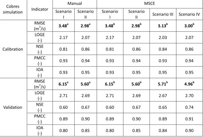
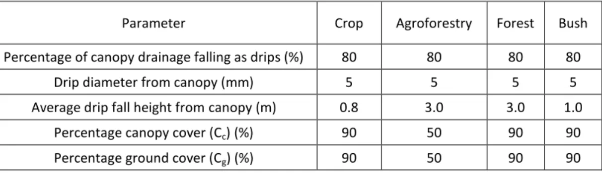
Table 3.1 Available TSS, turbidity and hourly discharge at Monte da Ponte gauging station ... 13 Table 3.2 Summary statistics for the data sets shown in Table 3.1 ... 14 Table 5.1 Comparison of model performances from manual and MSCE calibrations at basin outlet (Monte da Ponte gauging station) ... 29 Table 5.2 Description of SHETRAN key hydrological parameters, feasible ranges, baseline setting (in bracket) and values derived from manual and MSCE calibrations for different scenarios (I, II, III and IV) as explained in the Section 5.5.2 ... 31 Table 5.3 Comparison of model performances from manual and MSCE calibrations at basin outlet (Monte da Ponte gauging station) ... 36 Table 5.4 Statistics for the MSCE calibration scenario IV at Cobres basin ... 37 Table 5.5 Vegetation parameters for sediment transport simulations of Cobres basin . 54 Table 5.6 Soil textural data from Cardoso (1965) for soil types in Cobres basin ... 54 Table 5.7 Soil particle-size distribution for soil types in Cobres basin ... 55 Table 5.8 Mass fraction for sediment particle-size distribution of soil types in Cobres basin ... 55 Table 5.9 Preliminary sediment simulations of Cobres basin for the period from October, 2004 to November, 2006 ... 57 Table 5.10 Statistics of annual rainfall and runoff at Cobres basin ... 58 Table 6.1 Area, total river length and drainage density of the Cobres basin ... 69 Table 6.2 The SHETRAN key hydrological parameters derived from calibrations at Cobres basin with spatial resolution of 1.0 km and 2.0 km ... 75 Table 6.3 Comparison of the model performances for the SHETRAN simulations at Cobres basin with spatial resolutions of 1.0 km and 2.0 km ... 81 Table 6.4 Comparison of model performances for SHETRAN validation simulations at Albernoa basin with spatial resolutions of 1.0 km and 2.0 km ... 83 Table 6.5 Observed characteristics of the 11 selected “large storm events” at Cobres basin ... 85 Table 7.1 Characteristics of the stations located in the study area ... 94 Table 7.2 The Regional Climate Model (RCM) experiment used from the RT3 ENSEMBLES ... 98
xx
Table 7.3a Climate change impacts on moderate precipitation extreme indices (5th percentile) ... 119 Table 7.3b Climate change impacts on moderate precipitation extreme indices (50th percentile) ... 120 Table 7.3c Climate change impacts on moderate precipitation extreme indices (95th percentile) ... 120 Table 7.3d Climate change impacts on moderate precipitation extreme indices (98th percentile) ... 120 Table 8.1 Statistics for evaluation of climate change impacts on catchment: average changes in mean, standard deviation (STD), coefficient of variation (CV), 5th, 50th, 95th 98th and 99th percentiles (q0.05, q0.50, q0.95, q0.98 and q0.99) for annual rainfall (P), PET,
AET, subsurface storage (∆S), runoff (R) and sediment yield (SY) ... 130 Table 8.2a Lilliefors test for annual maximum daily discharge under CTL and FUT conditions ... 141 Table 8.2b Filliben test for annual maximum daily discharge under CTL and FUT conditions ... 141 Table 8.3a Lilliefors test for annual max daily sediment discharge under CTL and FUT conditions ... 141 Table 8.3b Filliben test for annual max daily sediment discharge under CTL and FUT conditions ... 141 Table A1.1 Description of SHETRAN key hydrological parameters for the simulations of the baseline and scenarios for sensitivity analysis ... 164 Table A1.2 Comparison of model performances from the SHETRAN simulations of the baseline and scenarios, with key parameters indicated in the Table A1.1 ... 165
xxi
List of Symbols and Abbreviations
List of Symbols
a Coefficient of the Yalin equation A Flow cross sectional area (m2)
AET Actual Evapotranspiration (mm) or (mm/s) AETPETFC1 The AET/PET ratio at field capacity for crop
AETPETFC2 The AET/PET ratio at field capacity for agroforestry
AII Average dry day precipitation (DP < 10 mm) (mm)
α van Genuchten α parameter (cm-1)
α1 van Genuchten α parameter of Vx soil (cm-1)
α2 van Genuchten α parameter of Px soil (cm-1)
α3 van Genuchten α parameter of Ex soil (cm-1)
αg,i Change factor for the statistic g and the calendar month i
αT,i Change factor for the temperature statistic T and the calendar
month i
b Drainage parameter
B Channel flow width (m) or active bed width for which there is sediment transport (m)
ci Sediment concentration in size group i (m3/m3)
cP Specific heat of air at constant pressure (J/kg/K)
C Depth of water on canopy (mm)
CDD Maximum number of consecutive dry days (DP < 1.0 mm) (day)
Cc Percentagecanopy cover (%)
Cg Proportion of ground shielded by near ground cover (decimal
fraction) or percentageground cover (%)
Cr Proportion of ground shielded by ground level cover (decimal
fraction)
CR Storm runoff coefficient (%)
D50 Sediment particle diameter greater than the diameter of 50% of
the particles (m);
Dn The largest absolute difference between empirical and fitted
cumulative probabilities
δ Coefficient of the Yalin equation δe Vapour pressure deficit of air (Pa)
xxii
Δ Rate of increase with temperature of the saturation vapour pressure of water at air temperature (Pa/K)
ΔS Change of subsurface water storage (mm)
Di Representative sediment particle diameter for the size group i
(m).
DP Daily precipitation (mm)
Dq Rate of detachment of soil per unit area (kg/m2/s)
Dr Rate of detachment of soil (kg/m2/s);
ei White noise on the day i for the equations 7.10─7.24 and
A2.1─A2.13
η Storage coefficient (m-1)
ηc Crossover distribution index
ηm Mutation distribution index
Eb Rate of detachment of material per unit area of river bank
(kg/m2/s)
Ex Lithosols from semi-arid and sub-humid climate of Schist or
Greywacke origin
FDD Number of dry spells (consecutive period with at least 8 dry days, DP < 1.0 mm) (freq.)
ηc Crossover distribution index
ηm Mutation distribution index
ϕ Bed sediment porosity (m3/m3)
Fw Effect of surface water layer in protecting the soil from raindrop
impact (dimensionless)
g Acceleration due to gravity (m/s2)
γ Psychrometric constant (~66 Pa/K)
𝑔𝑖𝐹𝑢𝑡, 𝑔
𝑖𝐶𝑜𝑛 The statistic g for the calender month i under the future (Fut) and
control (Con) conditions
𝑔𝑖𝑂𝑏𝑠, 𝑔𝑖𝐸𝑠𝑡 The observed (Obs) and estimated (Est) statistic g for the calender month i
Ggr,i Dimensionless sediment transport rate for sediment size group i
Gi Volumetric sediment transport rate for particles in size group i
(m3/s)
Gtot The capacity particulate transport rate for overland flow (including
all sediment size groups) (m3/s)
gx, gy Volumetric sediment transport rates per unit width in the x and y
xxiii
h Water depth (m) or top soil depth (m)
H Flow depth of channel flow (m)
HP Hourly precipitation (mm)
Imean Mean rainfall intensity (mm/h)
Imax Max rainfall intensity (mm/h)
k Drainage parameter
kb Bank erodibility coefficient (kg/m2/s)
kf Overland flow soil erodibility coefficient (kg/m2/s)
kr Raindrop impact soil erodibility coefficient (J-1) or relative
hydraulic conductivity (-)
K1 (m1/3/s) Strickler overland flow resistance coefficient for crops
K2 (m1/3/s) Strickler overland flow resistance coefficient for agroforestry
Ks Saturated hydraulic conductivity (m/day)
Ks1 Saturated hydraulic conductivity of Vx soil (m/day)
Ks2 Saturated hydraulic conductivity of Px soil (m/day)
Ks3 Saturated hydraulic conductivity of Ex soil (m/day)
Kx, Ky and Kl Strickler coefficients (m1/3/s), which are the inverse of the
Manning coefficient, in the x, y and l directions
Kx, Ky and Kz Saturated hydraulic conductivities in the x, y and z directions (m/s)
l Width of the flow (m)
L1ACDP Lag-1 autocorrelation (-)
λ Loose sediment porosity (decimal fraction) or latent heat of vaporization of water (J/g)
Md Momentum squared of leaf drips reaching the ground per unit
time per unit area (kg2/s3)
MDP Daily mean rainfall for a specified month (mm)
MDT Mean of daily mean 2-m air temperature for a specified month
(°C)
M∆DT Mean of daily 2-m air temperature range for a specified month
(°C)
Mr Momentum squared of raindrops reaching the ground per unit
time per unit area (kg2/s3)
n Porosity (m3/m3) or van Genuchten n parameter (-) n1 van Genuchten n parameter of Vx soil (-)
n2 van Genuchten n parameter of Px soil (-)
xxiv
ni The transition exponent for sediment size group i for the
Ackers-White equation for Channel flow sediment transport
Oi Observed watershed responses at time point i
𝑂̅ The mean values of observed watershed responses PET Potential Evapotranspiration (mm)
Ψ Soil moisture tension (m)
Ψw Soil moisture tension at wilting point (m)
ΨL Soil moisture tension at which soil water begins to limit plant
growth and water uptake is considered to take place at the potential rate (m)
P Precipitation (mm) or non-exceedance probabilities (-) PdryDP1.0 Proportion of dry days (less than 1.0 mm) (-)
PdryHP0.1 Proportion of dry hours (less than 0.1 mm) (-)
Pi Daily precipitation (mm) for the day i
Pobs Observed precipitation (mm)
Px Brown Mediterranean soil of Schist or Greywacke origin
q Specific volumetric flow rate out of the medium (s-1)
qsi Sediment input from bank erosion and overland flow supplies per
unit channel length for size fraction i (m3/s/m)
qw, qsp and qt Specific volumetric fluxes (s-1) out of abstraction well, spring
discharges and transpiration losses respectively
Q Net rate of rainfall supply to canopy (mm/hour) or water flow rate (m3/s)
Qb Baseflow ( at the start of the flood) (m3/s)
Qi Lateral influx (m3/s)
Qobs Observed discharge (m3/s)
Qp Peakflow (maximum peakflow for processes with multiple peaks)
(m3/s)
QR Net vertical input to the element (m3/s)
Qobs Observed discharge (m3/s)
Qsim Simulated discharge (m3/s)
𝑄𝑜𝑏𝑠𝑝𝑘 Observed peak discharges (m3/s) 𝑄𝑠𝑖𝑚𝑝𝑘 Simulated peak discharges (m3/s)
ra Aerodynamic resistence to water vapour transport (s/m)
rc Canopy resistance to water vapour transport (s/m).
xxv
ρs Density of sediment particles (kg/m3)
R Daily 2-m air temperature range (°C) or runoff (mm) or Pearson correlation coefficient (-)
R5D Highest consecutive 5-day precipitation total (mm)
R30 Number of days with daily precipitation totals above or equal to 30 mm (day)
Ri Daily 2-m air temperature range for the day i (°C)
Rn Net radiation (W/m2)
Robs Observed runoff (mm)
Rsim Simulated runoff (mm)
s Sediment specific gravity (decimal fraction)
S Water surface slope in the direction of flow (m/m) or canopy storage capacity (mm)
Si Simulated watershed responses at time point i
𝑆̅ The mean values of simulated watershed responses SDII Average wet day precipitation (DP >= 1.0 mm) (mm)
Sfx, Sfy and Sfl Friction slopes in the x, y and l directions respectively (m/m)
σe Standard deviation of the white noise on the day i for the
equations 7.10─7.24 and A2.1─A2.13
SkewDP Skewness of daily rainfall for a specified month (-)
SkewHP Skewness of hourly rainfall for a specified month (-)
Ss Specific storage (m-1)
SS Sunshine duration (hours)
SSi Sunshine duration for the day i (hours)
SY Sediment Yield (t ha-1 year-1)
t Time (hour or second)
T Daily mean 2-m air temperature (°C) or return period (year) θ Volumetric soil water content (m3/m3)
θs Saturated soil water content (m3/m3)
θs1 Saturated soil water content of Vx soil (m3/m3)
θs2 Saturated soil water content of Px soil (m3/m3)
θs3 Saturated soil water content of Ex soil (m3/m3)
θr Residual soil water content (m3/m3)
θr1 Residual soil water content of Vx soil (m3/m3)
θr2 Residual soil water content of Px soil (m3/m3)
θr3 Residual soil water content of Ex soil (m3/m3)
xxvi 𝑇𝑖𝐹𝑢𝑡, 𝑇
𝑖𝐶𝑜𝑛 The temperature statistic T for the calender month i under the
future (Fut) and control (Con) conditions
𝑇𝑖𝑂𝑏𝑠, 𝑇𝑖𝐸𝑠𝑡 The observed (Obs) and estimated (Est) temperature statistic T for the calender month i
Tmax Daily maximum 2-m air temperature (°C)
Tmin Daily minimum 2-m air temperature (°C)
τ Shear stress due to overland flow (N/m2) τb Shear stress acting on the bank (N/m2);
τbc Critical shear stress for initiation of motion of bank material (N/m2)
τec Critical shear stress for initiation of sediment motion (N/m2)
TSS Total suspended solid (mg/l)
Turb Turbidity (NTU)
ux, uy and ul Flow velocities in the x, y and l directions (m/s)
u* Shear velocity of channel flow (m/s)
U Water velocity of channel flow (m/s)
VarDP Variance of daily rainfall for a specified month (mm2)
VarDT Variance of daily mean 2-m air temperature for a specified month
(°C2)
Var∆DT Variance (Var∆DT) of daily 2-m air temperature range for a
specified month (°C2)
VarHP Variance of hourly rainfall for a specified month (mm2)
VP Vapour pressure (kPa)
VPi Vapour pressure for the day i (kPa)
Vx Yellow Mediterranean soil of Schist origin
WS Wind speed (m/s)
WSi Wind speed for the day i (m/s)
XCDP Spatial cross correlation between the rain gauges (-)
X(Pdry) The invertible transformation X that can be applied to the
proportional dry variable Pdry
Y(L1AC) The invertible transformation Y that can be applied to the lag-1
autocorrelation variable L1AC
z Depth of loose soil (m) or z = depth of bed sediment (m)
zg Ground or channel bed level (m)
List of Abbreviations
xxvii
Additive Ɛ-indicator The largest distance required to translate the approximation set solution to dominate its nearest neighbor in the best known approximation set
Alb Albernoa
Alm Almodôvar
AOGCM Atmposphere-ocean coupled general circulation model
Bej Beja
Cas Castro verde
CDF Cumulative distribution function
CF Change Factor
CLEMDES Clearing house mechanism on desertification for the Northern Mediterranean region, an European project with the aim of setting up an Internet based network devoted to the improvement of the diffusion of information among public.
CORDEX COordinated Regional climate Downscaling Experiment, a WCRP (World Climate Research Programme) sponsored program to produce regional climate change scenarios globally, contributing to the IPCC’s fifth Assessment Report (AR5) and to the climate community beyond the AR5.
CORINE Coordination of information on the environment Crit0.05 The critical value at a significance level of 5%
CRU-WG Climate Research Unit daily Weather Generator
CTL Control
CV Coefficient of Variation
DEM Digital Elevation Model
DesertWATCH An European Space Agency (ESA) project aiming at developing a user-oriented Information System based on EO technology to support national and local authorities in responding to the reporting obligations of the UNCCD and in monitoring land degradation trends over time.
DESERTLINKS An European, international and interdisciplinary research project funded by the European Commission under Framework Programme 5, with the aim of developing a desertification indicator system for Mediterranean Europe
DeSurvey A project funded by the European Commission under the Framework Programme 6 and contributing to the implementation of the actions 'Mechanisms of desertification' and 'Assessment of
xxviii
the vulnerability to desertification and early warning options' within the 'Global Change and Ecosystems priority'
DISMED Desertification Information System for the Mediterranean, an European project to improve the capacity of national administrations of Mediterranean countries to effectively program measures and policies to combat desertification and the effects of drought.
E Exponential distribution
EEA European Environment Agency, www.esa.int
ENSEMBLES An EU-FP6 financed project. The value, and core, of the ENSEMBLES project is in running multiple climate models (‘ensembles’); a method known to improve the accuracy and reliability of forecasts.
ERLAND A research project financed by FCT for estimating the impacts of climate change on soil erosion in representative Portuguese agroforestry watersheds, due to changes in rainfall, runoff generation and vegetation cover.
ESA European Space Agency
EU-FP6 European Union Sixth Framework Programme,
http://ec.europa.eu/research/fp6/index_en.cfm
EV Gumbel or Extreme Value distribution
EXP Expected
FAO Food and Agriculture Organization, www.fao.org
FCT Fundação para a Ciência e a Tecnologia, http://www.fct.pt/, (Portuguese national funding agency for science, research and technology)
FUT Future
G Gumbel distribution
GA Genetic Algorithm
GCM Global Climate Model
GDP Gross domestic product
Generational distance The average Euclidean distance of points in an approximation set to their nearest corresponding points in the best known approximation set.
GEV Generalized Extreme Value
GHGs Green House Gases
xxix
GNO The generalized normal distribution GPA The generalized Pareto distribution
GW Groundwater model
HydroGeoSphere A fully integrated, physically based hydrological model
Hypervolume The ratio of volume of objective space dominated by an approximation set to that dominated by the best known approximation set
HH:MM Hours:Minutes
ICAAM-WG The Institute of Mediterranean Agricultural and Environmental Sciences daily Weather Generator
IHERA Instituto de Hidráulica, Engenharia Rural e Ambiente (Institute of Hydraulics, Rural Engineering and Environment)
ln3 Three-parameter lognormal distribution
IOA Index of agreement
IP Iberian Peninsula
IPCC Intergovernmental Panel on Climate Change, http://www.ipcc.ch/ IPMA Instituto Português do Mar e da Atmosfera, www.ipma.pt,
(Portuguese Institute for the Ocean and Atmosphere)
IQRs Interquartile Ranges
ISD Indicator of Susceptibility to Desertification
L Logistic distribution
LADAMER Land Degradation Assessment in Mediterranean Europe, an European project with the aim of providing an assessment of the degradation status of Mediterranean lands on small scales, and the identification of Hot Spot areas subject to high desertification and land degradation risk
LAMs Limited-area models
LHS Latin hypercube sampling
LOG Logarithm
LOGE LOG transformed Error
LUCINDA Land care in desertification affected areas: from science towards application, an European project with aim of promoting and facilitating the dissemination, transfer, exploitation and broad take-up of past and present research programme results in the theme of combating desertification in Mediterranean Europe.
MBE Mass Balance Error
xxx
MEDACTION An European Commission funded 5th Framework Program research project that aims to address the main issues underlying the causes, effects and mitigation options for managing land degradation and desertification in the North Mediterranean region of Europe.
MEDALUS Mediterranean Desertification and Land Use, an international research project with the general aim to investigate the relationship between desertification and land use in Mediterranean Europe.
MCCE Modified Competitive Complex Evolution
METO-HC_HadRM3Q0 The Met Office Hadley Centre regional climate model HadRM3Q0 with normal sensibility
MIKE SHE An integrated hydrological modelling system for building and simulating surface water flow and groundwater flow
MOEA Multi-Objective Evolutionary Algorithms Monte Ponte Monte da Ponte gauging station
MOSCEM-UA Multi-Objective Shuffled Complex Evolution Metropolis global optimization algorithm
MRC Modelo Regional Climático
MSCE Modified Shuffled Complex Evolution
N Normal distribution
NAO North Atlantic Oscillation
NOPT The number of optimization parameters NSE Nash-Sutcliffe Efficiency
NSGA-II Non-dominated sorting genetic algorithm II
OBS Observation or observed
Opt-indicator The smallest distance required to translate the approximation set solution to dominate its nearest neighbor in the best known approximation set
PBSD Physically-based spatially-distributed PDF Probability density function
PE3 The Pearson type III distribution
PKE Peak Error
PM Polynomial mutation
PMCC Coefficient of determination
xxxi
PRUDENCE Prediction of Regional scenarios and Uncertainties for Defining EuropeaN Climate change risks and Effects, an European Union project with the aim of providing high resolution climate change scenarios for Europe at the end of the twenty-first century by means of dynamic downscaling (regional climate modelling) of global climate simulations.
q0.05, q0.25, q0.50, q0.75, q0.95 q0.98 and q0.99 5th, 25th, 50th, 75th, 95th, 98th and 99th
percentile
RainSim V3 Rainfall simulation version 3 model
RCM Regional Climate Model
RCPs Representative Concentration Pathways, which are four greenhouse gas concentration trajectories adopted by the IPCC for its fifth Assessment Report (AR5) in 2014
REACTION Restoration actions to combat desertification in the Northern Mediterranean, an European project with its general objective of facilitating access to high quality information for forest managers, scientists, policy-makers and other stakeholders, providing tools for the promotion of techniques and initiatives for sustainable mitigation actions
RMSE Root Mean Square Error
SAC-SMA Sacramento Soil Moisture Accounting model, a conceptual hydrological model that attempts to represent soil moisture characteristics to effectively simulate runoff that may become streamflow in a channel
SAGRA/COTR Sistema Agrometeorológico para a Gestão da Rega no Alentejo/ Centro Operativo e de Tecnologia de Regadio,
http://www.cotr.pt/cotr/sagra.asp, (the Portuguese
Agrometeorological System for the Management of Irrigation in the Alentejo/Irrigation Technology and Operative Center)
Sao São Marcos da Ataboeira
SAO MDA São Marcos da Ataboeira station
Sbp Santa Barbara de Padrões
SBX Simulated binary crossover
SCE Shuffled Complex Evolution
SCE-UA Shuffled Complex Evolution method developed at the University of Arizona
xxxii
SHETRAN Système Hydrologique Européen TRANsport, a physically-based spatially-distributed modelling system for water flow and sediment and contaminant transports in river catchments,
http://research.ncl.ac.uk/shetran/
SIM Simulation or simulated
SNIRH Sistema Nacional de Informação de Recursos Hídricos,
www.snirh.pt, (Portuguese national water resources information
system)
SPEA2 The Strength Pareto Evolutionary Algorithm 2 SRES Special Report on Emissions Scenarios
STD Standard deviation
STNSRP Spatial Temporal Neyman-Scott Rectangular Pulse
SWAT Soil and Water Assessment Tool, a river basin scale model developed to quantify the impact of land management practices in large, complex watersheds
Trindade Tri
U Uniform distribution
UNCCD United Nations Convention to Combat Desertification,
www.unccd.int
Vdc Vale de Camelos
WESP Watershed Erosion Simulation Program
WetSpa Water and Energy Transfer between Soil, Plants and Atmosphere, a distributed hydrological model for prediction of river discharges
WS Wind speed
1
1. Introduction and Objectives
Semi-arid (EEA 2012), large intra- and inter-annual variability in precipitation (Corte-Real et al., 1998; Mourato et al., 2010; Guerreiro et al., 2014), drought (Santos et al., 2010), land abandonment, land degradation (Pereira et al., 2006) and desertification (Rubio and Recatalà 2006) have been the highlights of southern Portugal since the early 1990s (Bathurst et al., 1996; Thornes 1998). Water shortage and desertification processes are the main problems the region is confronting. The persistence of temperature rise and precipitation decrease has exacerbated the situation (EEA 2012; IPCC 2013), which will continue to be at stake in the 21st century (Kilsby and Tellier
et al., 2007; Mourato 2010; EEA 2012; IPCC 2013). Mitigation strategies are urgently
required to make the region sustainable for the future climate change impacts (IPCC 2012); and a step of utmost importance is the accurate quantification of water availability and extreme events for both current and future climates. Recent studies from EEA 2012, Feyen et al. (2012), Rojas et al. (2012), Rojas et al. (2013), Rajczak
et al. (2013) and Schneider et al. (2013) have dealt with the issues at a spatial level of
European continent; however, their results cannot be extracted for a direct use at a catchment scale of southern Portugal due to the considered coarse spatial resolutions. Among investigations on climate change impacts of the region, some regarded only the changes in precipitation (Corte-Real et al. 1995b, 1998, 1999a and 1999b), and others have not included recent progresses in regional climate modelling, downscaling methods and hydrological models as well as observation data with temporal resolution higher than a day (Bathurst et al., 1996; Bathurst and Bovolo 2004; Kilsby and Tellier
et al., 2007; Mourato 2010). The present study attempts to fill the mentioned gaps.
The objective of this study is to investigate the climate change impacts on the agricultural dominated Cobres basin in southern Portugal in terms of water resources, extreme events as well as sediment transport, considering the importance of sediment yield in the risk of desertification which has been demonstrated by Vanmaercke et al. (2011). The selection of Cobres basin as the study area can be justified by the problems of southern Portugal described in Section 2.1 as well as by previous studies of MEDALUS and MEDACTION projects. The study, sets 1981–2010 as the control period, due to the data availability, and 2041–2070 as the future period for practical purpose. Considering the size and topography of the Cobres basin, hourly precipitation and daily potential evapotranspiration (PET) are enough for getting better representation of hydrological and sediment transport processes under both control
2
and future climates. The state-of-the-art climate projections derived from the RCM HadRM3Q0 output, provided by the ENSEMBLES project (van der Linden et al., 2009), together with the advanced version of the Spatial-Temporal Neyman-Scott Rectangular Pulses (STNSRP) model RainSim V3 (Burton et al., 2008) are used to downscale synthetic hourly precipitation series. Daily PET is calculated based on the FAO Penman-Monteith equation (Allen et al., 1998) and the variables, namely daily maximum and minimum 2-m air temperatures, sunshine duration hours, vapour pressure and wind speed, are generated by the rainfall conditioned weather generator—ICAAM-WG, developed in this study, based on the modified Climate Research Unit daily Weather Generator (CRU-WG) (Kilsby and Jones et al., 2007). Temperature variables are projected to change based on the RCM HadRM3Q0 output; other variables are assumed not to change for future, because maximum sunshine duration cannot increase, and vapour pressure and wind speed are projected with large uncertainties, differing largely from the different RCM integrations (van der Linden et al., 2009). Bias of RCMs statistics for precipitation and temperature are corrected based on the change factor approach described in Kilsby and Jones et al. (2007) and Jones et al. (2009). The physically-based spatially-distributed model SHETRAN (Ewen et al., 2000) is used for the simulations of hydrological and sediment transport processes. A global optimization method is used for automatically getting the best parameter setting in their physically constrained ranges; and the effects of spatial resolutions on SHETRAN performance are also investigated. Finally, three series of 1000-year hydrological and sediment transport processes are developed, respectively for control and future climates, to provide a robust conclusion.
The structure of the thesis is as follows: Chapter 2 shows the scientific background of the present study. Chapters 3 and 4 respectively introduce the study area and data preparation processes and the SHETRAN hydrological modelling system. Chapters 5 and 6 provide the bases of SHETRAN model set-up. To be specific, Chapter 5 demonstrates automatic calibrations of SHETRAN model by using two global optimization methods; and Chapter 6 investigates the effects of spatial resolution on SHETRAN model performance. Chapter 7 is dedicated to prepare the series of synthetic hourly precipitation and daily PET for both control and future climates. Chapter 8 assesses future climate change impacts on Cobres basin. Finally, Chapter 9 concludes the study and suggests recommendations for further research.