The implementation of the Basel III Countercyclical Capital Buffer in Portugal

(1)

The implementation of the Basel III Countercyclical Capital Buffer

in Portugal

Rui Fonseca

Advisor: Diana Bonfim

Dissertation submitted in partial fulfillment of requirements for the degree of Master in

Finance, at the Universidade Católica Portuguesa, November 2013

(2)

Rui Fonseca ii

Abstract

Basel II capital requirements are risk sensitive because they rely on the credit quality of borrowers, which means that in a downturn of the business cycle, when capital might be needed to absorb losses, capital requirements are also expected to be higher. This procyclicality may lead to excessive risk-taking during good times and to a credit crunch during bad times, amplifying the business cycle effects. Several approaches were proposed to address this problem.

The new Basel III framework directly addresses this issue, mainly through the implementation of the countercyclical capital buffer. This buffer aims to protect the banking system from periods of excessive credit growth, ensuring that the financial sector, as a whole, has enough capital to maintain the flow of credit into real economy in stress periods and that capital requirements do not constraint credit supply.

The objective of this thesis is to discuss the implementation in Portugal of the Basel III countercyclical capital buffer framework. The analysis was organized in two main parts, answering two different questions.

First, the historical performance of the common guide Credit-to-GDP gap, proposed by the Basel Committee on Banking Supervision (BCBS) to signal the built up of the countercyclical capital buffer, was tested. The results showed that the guide can signal the build up of the buffer complying with the objectives set. However, according to the results, some alterations to the methodology proposed may need to be considered, in order to improve the calibration for the Portuguese economy. For instance, a smoothing parameter of 1 600 instead of 400 000 to compute the trend using a recursive Hodrick-Prescott filter may provide better results, while changing the lower and upper thresholds might also be necessary.

The second objective was to assess if Portuguese banks would respond to an increase of capital requirements by constraining loan supply or by other means. To do so it was used an approach based on the previous work of Francis and Osborne (2012), which studied the effects of regulatory capital requirements on capital, lending and balance sheet management of UK banks. The results suggest that Portuguese banks tend to react to capital requirement increases by raising the levels of regulatory capital.

(3)

Rui Fonseca iii

Acknowledgements

This thesis represented a challenge, not only because of its own difficulties, but also because it was accomplished while I was father of my second child, which was demanding, and I also had to maintain my professional obligations. Obtain the data needed was the most defying task, being responsible for a delay in the completion of the work.

The support of my family, especially my wife which was restless during this endeavor, was essentially.

I also would like to sincerely thank my advisor, Diana Bonfim, for her support and total availability during this process.

(4)

Rui Fonseca iv

1 Introduction

Banking system regulators impose minimum capital ratios to banks, which depend on the coverage of risk weighted assets (RWA) by the level of own funds held by the institution. Basel II capital requirements, in place today, are risk sensitive because RWA depend on the credit quality of borrowers. This means that in a downturn of the business cycle, when overall credit quality decreases, RWA tend to be higher and in good times tend to be lower for the exact opposite reasons. This procyclicality gives a wrong incentive to banks that may lead to excessive risk-taking during good times and to a credit crunch during bad times, amplifying the business cycle effects.

This problem led to the necessity of presenting solutions to smooth the effects of procyclicality and, in consequence, several approaches were proposed. The new Basel III framework directly addresses this problem, mainly through the implementation of the countercyclical capital buffer, which aims to protect the banking system from periods of excessive credit growth, ensuring that the financial sector, as a whole, has enough capital to maintain the flow of credit into real economy in stress periods and that capital requirements do not constraint credit supply. To do so, this buffer should be imposed by national authorities if they believe to be in the presence of excessive credit growth that is contributing to the build up of system-wide risk (constraining it) and should be released in the presence of a crisis or when the risks identified subside. Although national authorities should apply proper judgment in buffer decisions, the variable Credit-to-GDP gap, explained afterwards, was proposed by the Basel Committee on Banking Supervision (BCBS) to be a common guide in signaling the build up of the countercyclical capital buffer.

The objective of this thesis is to discuss the implementation in Portugal of the Basel III countercyclical capital buffer framework. The analysis was organized in two main parts, answering two different questions.

First, the historical performance of the common guide Credit-to-GDP gap, proposed by the Basel Committee on Banking Supervision (BCBS) to signal the built up of the countercyclical capital buffer, was tested.

The second objective was to assess if Portuguese banks would respond to an increase of capital requirements by constraining loan supply or by other means. To do so it was used an

(6)

Rui Fonseca 6 approach based on the previous work of Francis and Osborne (2012), which studied the effects of regulatory capital requirements on capital, lending and balance sheet management of UK banks.

The rest of the document is organized as follows:

1. The second chapter will address the importance of capital and the evolution of international capital regulation. It will also address procyclicality in capital regulation and the role of the Basel III countercyclical capital buffer in mitigating it, while also reviewing some of the related literature;

2. The third chapter will explain how the common guide Credit-to-GDP will be implemented and assess its historical performance in Portugal;

3. The fourth chapter will analyze how Portuguese banks adjust their balance sheets to comply with changes in capital requirements;

4. Finally, conclusions are presented in the fifth chapter.

2 International capital regulation

2.1 Capital

It is common for financial institutions to incur in losses due to their activity and they must be prepared to absorb these losses in order to maintain themselves operating in the long run. The losses can be of different magnitude and probability, as shown in Figure 1, and should be dealt with in different ways. The expected loss, due to its high probability of occurring, should be covered by the regular activity with an adequate pricing of the products and provisioning, while the unexpected loss, which is not expected to be exceeded with some degree of confidence (usually 99% or 99.9%), should be absorbed by capital. This means that an adequate capital level prevents financial institutions from failure when extreme losses occur. The stress loss is the unexpected loss level which it is judged to be too expensive to hold capital against, meaning that this level of losses leads to insolvency.

(7)

Rui Fonseca 7

Figure 1 – The loss probability function

The failure of a financial institution may cause serious damage in the financial system where it is integrated and also in the real economy, due to the propagation of losses across banks, which in turn may lead to the default of other financial institutions (systemic risk) and to a reduction of the credit supplied to households and corporations, deteriorating the economy. In order to prevent these negative impacts on the financial system and economy, regulators must ensure that banks hold adequate levels of capital, preventing them from defaulting.

Before 1988, many regulators of different countries imposed minimum levels of capital coverage over total assets. However, the definitions of capital and minimum levels required were not homogeneous across jurisdictions, which lead to unequal conditions to banks competing worldwide, giving an edge to the ones with slack regulation. Additionally, due to the existence of new transactions accounted as off-balance sheet items (e.g. over-the-counter derivatives), the amount of capital required should not be based only on total assets, being required a better measure of the risks taken by banks.

2.2 Basel I

These constrains were behind the creation of the Basel Committee on Banking Supervision in 1974 and to the subsequent first approach to set international risk-based standards for capital adequacy (“The 1988 BIS Accord”). Despite of maintaining a minimum standard based on the ratio of capital to total assets, where banks were required to have a minimum multiple of 20, a

(8)

Rui Fonseca 8 new standard, based on the bank’s total credit exposure, was introduced and became known as the Cooke ratio.

The Cooke ratio consisted on the coverage of risk-weighted assets (RWA), which include off-balance sheet items, by total capital and a minimum of 8% was set. Total capital was composed by Tier 1 Capital, with a better loss-absorbing quality and a minimum requirement of 4%, and by Tier 2 Capital, also known as Supplementary Capital.

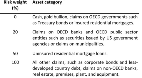
To compute the risk-weighted assets, a risk-weight was applied to each exposure based on the asset category, as shown in Table 1 (example for on-balance sheet items). The exposure of off-balance sheets items consisted in a credit equivalent amount, which for non-derivatives derived from applying a credit conversion factor (CCF) to the principal amount and for derivatives resulted from adding to the exposure an add-on factor, to reflect the possibility of increasing the exposure in the future (the add-on factor is a percentage of the principal and depends on the residual maturity of the position and the type of underlying).

Risk weight (%)

Asset category

0 Cash, gold bullion, claims on OECD governments such as Treasury bonds or insured residential mortgages. 20 Claims on OECD banks and OECD public sector

entities such as securities issued by US government agencies or claims on municipalities.

50 Uninsured residential mortgage loans.

100 All other claims, such as corporate bonds and less-developed country debt, claims on non-OECD banks, real estate, premises, plant, and equipment.

Table 1 – Risk weights for on-balance sheet items

In 1998, it was implemented the “1996 Amendment” to the original accord. This amendment introduced a capital requirement to cover exposures to market risks in addition to the existing capital requirement to cover exposures to credit risks. To calculate the market risk capital requirements, banks were allowed to use a standardized approach or an “internal model-based approach” (model-based on internal value-at-risk measurements), depending on the abilities of different banks in risk management. Most large banks preferred to use the latter model, because it led to lower capital requirements, due to diversification effects (Hull, 2010).

(9)

Rui Fonseca 9 Despite the advantages brought by the 1988 BIS Accord in the improvement of the level of capital held by banks and consequently in the stability of the banking system, its simplicity did not allow to capture well credit risk, because the risk weight to be applied to a position only depended on the asset class, ignoring the creditworthiness of the counterparty. In 1999 a new set of rules was proposed by the BCBS and the final set of what has become known as Basel II was published in 2004 and implemented in 2007.

2.3 Basel II

Basel II is based on three “pillars”, namely, (1) minimum capital requirements, (2) supervisory review and (3) market discipline. Concerning minimum capital requirements, two innovations relatively to the 1996 Amendment took place. First, the minimum capital requirement for credit risk reflects the credit rating of counterparties set by authorized External Credit Assessment Institutions (ECAI). Second, a new capital requirement for operational risk was established. This means that the total capital requirement under Basel II is

( )

Equation 1 – Capital requirements under Basel II

For credit risk measurement, institutions are allowed to choose from one of three available options:

1. The standardized approach;

2. The foundation internal ratings based (IRB) approach;

3. The advanced IRB approach.

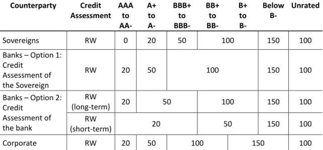
The standardized approach differs from Basel I in the additional risk sensitivity through the use of a wider range of risk weights linked to external ratings. As can be observed in Table 2, the risk weights depend not only on the counterparty class, but also on its rating.

(10)

Rui Fonseca 10 Counterparty Credit Assessment AAA to AA- A+ to A- BBB+ to BBB- BB+ to BB- B+ to B- Below B- Unrated Sovereigns RW 0 20 50 100 150 100 Banks – Option 1: Credit Assessment of the Sovereign RW 20 50 100 150 100 Banks – Option 2: Credit Assessment of the bank RW (long-term) 20 50 100 150 100 RW (short-term) 20 50 150 100 Corporate RW 20 50 100 150 100

Table 2 – Risk weights (as percentage of principal) under Basel II’s standardized approach

Under the IRB approach, capital requirements depend on the Probability of default (PD), Loss given default (LGD), Exposure at default (EAD) and Maturity adjustment (MA). For corporate, sovereign and bank exposures, under the foundation IRB approach, banks compute PD and the remaining risk parameters are set by the regulator, while under the advanced IRB approach, banks compute their own estimates of PD, LGD, EAD and MA. Under both IRB approaches, for the calculation of capital requirements for retail exposures, banks provide their own estimates of PD, LGD and EAD (in this case there is no maturity adjustment).

2.4 Basel III

On June 2011, it was published the final version of the original December 2010 Basel III document entitled “Basel III: A global regulatory framework for more resilient banks and banking systems”. This framework was designed to strengthen capital and liquidity rules in order to promote a more resilient banking sector, able to absorb shocks arising from financial and economic stress, and by doing so, reducing the risk of damaging the real economy.

These new rules also intend to reflect the lessons learned from the recent financial crisis, which began in 2007/2008. The main drivers of this crisis, according to the BCBS1, were the build up of excessive on- and off-balance sheet leverage, a gradual erosion of the level and quality of the capital base and also the insufficient liquidity buffers held by some banks. The

(11)

Rui Fonseca 11 crisis was also amplified by the procyclical deleveraging process and the linkage between systemic institutions, through complex transactions.

In order to address these problems, the framework’s main objectives are:

1. Raising the quality, consistency and transparency of the capital base; 2. Enhancing risk coverage;

3. Supplementing the risk-based capital requirement with a leverage ratio; 4. Reducing procyclicality and promoting countercyclical buffers;

5. Addressing systemic risk and interconnectedness; 6. Introducing a global liquidity standard.

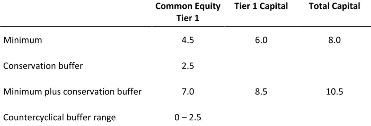
The new minimum capital requirements, as can be observed in Table 3, are imposed not only to Tier 1 Capital and Total Capital as in Basel II, but introduce the concept of Common Equity Tier 1 and two additional Capital buffers (the Conservation buffer and the Countercyclical buffer).

Common Equity Tier 1

Tier 1 Capital Total Capital

Minimum 4.5 6.0 8.0

Conservation buffer 2.5

Minimum plus conservation buffer 7.0 8.5 10.5

Countercyclical buffer range 0 – 2.5

Table 3 - Capital requirements and buffers (all numbers in percent)

The introduction of the capital requirements for Common Equity Tier 1 serves the objective of raising the quality of the capital base as it is basically composed by common shares and retained earnings. The capital conservation buffer, comprised of Common Equity Tier 1, intends to ensure that banks build up and maintain an excess of high quality capital outside of periods of stress, through the retaining of earnings, which can be used to absorb future losses. The countercyclical buffer is designed with the purpose of reducing procyclicality. This will be discussed in more detail on the next sections (section 2.5 discusses procyclicality and section 2.6 addresses the Basel III countercyclical capital buffer).

(12)

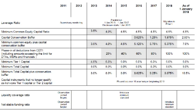
Rui Fonseca 12 The Basel III framework, which should be fully implemented in 1 January 2019, started its phase-in arrangements in 2013 as shown in Table 4.

Table 4 – Basel III phase-in arrangements

The CRD IV package transposes Basel III into the European Union legal framework and entered into force on 17 July 2013. Institutions are required to apply the new rules from the 1 January 2014, with full implementation on 1 January 2019 (European Commission).

2.5 Procyclicality

Basel II capital requirements are risk sensitive because they rely on the credit quality of borrowers, as mentioned before. Under the standard approach, the credit quality is reflected by the borrower’s external rating, when available, and under the IRB approach on the borrower’s probability of default. This means that in a downturn of the business cycle, when capital might be needed to absorb losses, capital requirements are also expected to be higher and, as shown in the work of Kashyap and Stein (2004), under the IRB approach this increase of the capital requirements might be substantial. This procyclicality may lead to excessive risk-taking during good times and to a credit crunch during bad times, amplifying the business cycle effects.

(13)

Rui Fonseca 13 According to the BCBS2, “one of the most destabilizing elements of the crisis has been the

procyclical amplification of financial shocks throughout the banking system, financial markets and the broader economy”. The BSBC also claims that “losses incurred in the banking sector can be extremely large when a downturn is preceded by a period of excess credit growth. These losses can destabilise the banking sector and spark a vicious circle, whereby problems in the financial system can contribute to a downturn in the real economy that then feeds back on to the banking sector.”

Although there is some agreement that the effect of procyclicality of the Basel II capital requirements should be mitigated and that it should be done without throwing out the risk-sensitiveness of capital regulation regime, different solutions were proposed by several authors.

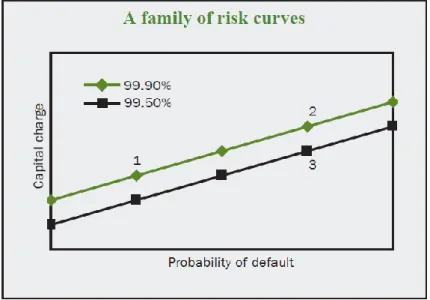
Kashyap and Stein (2004) argue that having a single time-invariant “risk curve”—that maps credit-risk measures (such as the PD) into capital charges—is, in general, suboptimal. These authors propose the use of several point-in-time risk curves (several confidence levels), as displayed in Figure 2, with each curve corresponding to different macroeconomic conditions (for the same probability of default, the capital charge should be lower in bad times of the business cycle). The authors suggest two equivalent ways of accomplishing the shift between curves, either by reducing the minimum capital ratio required in a recession or by a reduction of the risk weights assigned to loans of varying risk profiles.

Figure 2 – Kashyap and Stein (2004) Family of risk curves

(14)

Rui Fonseca 14 Repullo, Saurina, & Trucharte (2010) also show that Basel II capital requirements move significantly along the business cycle (more than 50% from peak to trough). Using the Basel II formula to calculate capital requirements, their analysis was based on an estimation of

point-in-time (PIT) PDs resulting from a logistic model of the one-year-ahead probabilities of default

of Spanish firms during the period 1987-2008. They also tested two different solutions to mitigate the cyclicality of these requirements over the business cycle. The first procedure consisted in smoothing the input of the Basel II formula by using some through-the-cycle (TTC) adjustment of the PDs and the second in smoothing the output of the formula computed from the PIT PDs. For the latter they tested different adjustments based on aggregate information (the rate of growth of the Gross Domestic Product (GDP), the rate of growth of bank credit, and the return of the stock market) and on individual bank information (the rate of growth of banks’ portfolios of commercial and industrial loans). The results showed that the best procedures are either to smooth the input of the Basel II formula by using TTC PDs or to smooth the output with a multiplier based on GDP growth. They also concluded that the latter solution is better in terms of simplicity, transparency, and consistency with banks’ risk pricing and risk management systems.

Another approach to deal with the problem is through countercyclical bank capital buffers that mitigate bank procyclicality in credit supply. In Spain the build up of these buffers is accomplished by the use of dynamic provisions, which are not related to bank specific losses and are forward-looking provisions, allowing the build up of a buffer from retained profits in good times that can then be used to cover the realized losses in bad times (Jiménez, Ongena, Peydró, & Saurina, 2013). Dynamic provisions are formula based, being the total loan loss provisions for a period (flow) the sum of the Specific plus General Provisions. General

Provisions are computed by the following formula:

(

)

Equation 2 – General provisions simplification formula in Spain (Jiménez, Ongena, Peydró, & Saurina, 2013)

where is the stock of loans at the end of period and its variation from the end of period to the end of period (positive in a lending expansion, negative in a credit decline). and are parameters set by the Banco de España ( is an estimate of the percent latent loss in the loan portfolio, while is the average along the cycle of specific provisions in relative terms.

(15)

Rui Fonseca 15 Jiménez, Ongena, Peydró, & Saurina (2013) studied the effects of dynamic provisioning in Spain in the period between 1999 and 2010 and concluded that the buffering stemming from it reduces credit supply in good times (when more risk creeps into bank balance sheets) and supports bank lending in bad times, with less need for costly governmental bail-outs and/or expansive monetary policy.

2.6 Basel III Countercyclical Capital Buffer

The Basel III framework also addresses this problem by the implementation of the countercyclical buffer, which aims to protect the banking system from periods of excessive credit growth, ensuring that the financial sector, as a whole, has enough capital to maintain the flow of credit into real economy in stress periods and that capital requirements do not constraint credit supply.

The buffer, to be filled with Common Equity Tier3, should be imposed by national authorities if they believe to be in the presence of excessive credit growth that is contributing to the build up of system-wide risk. It will assume values within the range of zero to 2.5% of risk weighted assets4 and extends the magnitude of the conservation buffer, as presented in Table 5.

Common Equity Tier 1 Ratio

(including other fully loss absorbing capital)

Minimum Capital Conservation Ratios (expressed as a percentage of earnings)

4.5% - 5.75%

(within 1st quartile of buffer) 100%

>5.75% - 7.0%

(within 2nd quartile of buffer) 80%

>7.0% - 8.25%

(within 3th quartile of buffer) 60%

>8.25% - 9.5%

(within 4th quartile of buffer) 40%

> 9.5%

(Above top of buffer) 0%

Table 5 - Individual bank minimum capital conservation standards, when a bank is subject to a 2.5% countercyclical requirement

3

For the moment only Common Equity Tier 1 should be used to meet the buffer. However, the Committee is reviewing the possibility of allowing other forms of capital.

4

National authorities can implement a range of additional macroprudential tools, including a buffer in excess of 2.5% for banks in their jurisdiction, if this is deemed appropriate in their national context. However, the international reciprocity provisions set out in this regime treat the maximum countercyclical buffer as 2.5%.

(16)

Rui Fonseca 16 The specific buffer requirement for each bank is based on a weighted average of the capital buffers determined by each jurisdiction where the bank has credit exposure (Basel Committee on Banking Supervision, 2010).

Increases in the countercyclical buffer will have to be announced at least a year earlier, in order to assure that banks have enough time to comply with the new capital requirements. On the contrary, decreases in the buffer may take effect immediately to mitigate the risk of credit crunches due to higher capital requirements imposed by regulators (Basel Committee on Banking Supervision, 2010).

It is expected for authorities to define an internationally common guide for the buffer that can be a starting point for decisions concerning the buffer. The Bank for International Settlements presents an extensive analysis of the properties of a broad range of indicator variables and the credit-to-GDP gap had the best performance. Another advantage of this indicator is being based on credit, as constraining excessive credit growth is also an objective of the countercyclical capital buffer. This guide does not always work well in every jurisdiction, and that is why judgment has an important role in this regime. In order to guide authorities in their judgment, the BCBS defined a set of principles included in the document Guidance for national

authorities operating the countercyclical capital buffer (Basel Committee on Banking

Supervision, 2010), as follows:

1. Objectives: “Buffer decisions should be guided by the objectives to be achieved by the

buffer, namely to protect the banking system against potential future losses when excess credit growth is associated with an increase in system-wide risk.”

2. Common reference guide: “The credit/GDP guide is a useful common reference point in

taking buffer decisions. It does not need to play a dominant role in the information used by authorities to take and explain buffer decisions. Authorities should explain the information used, and how it is taken into account in formulating buffer decisions.”

3. Risk of misleading signals: “Assessments of the information contained in the credit/GDP

guide and any other guides should be mindful of the behaviour of the factors that can lead them to give misleading signals.”

(17)

Rui Fonseca 17 4. Prompt release: “Promptly releasing the buffer in times of stress can help to reduce the

risk of the supply of credit being constrained by regulatory capital requirements.”

5. Other macroprudential tools: “The buffer is an important instrument in a suite of

macroprudential tools at the disposal of the authorities.”

With the objective of giving credibility to the buffer decisions, authorities should disclose the information used in the process. It is also important that capital buffer decisions should be updated frequently to mitigate the risk of the buffer not being in line with the credit cycle (the BCBS suggests reviews on a quarterly or more frequent basis (Basel Committee on Banking Supervision, 2010)).

3 Credit-to-GDP

In the document Guidance for national authorities operating the countercyclical capital buffer is presented a series of graphics for several countries which allows observing the past performance of the credit-to-GDP gap as a signaling variable for the buffer decisions and for most of the countries this indicator performed well. In this chapter will be presented some conclusions presented by several authors regarding the performance of the credit-to-GDP gap and its historical performance in Portugal will be assessed.

Repullo and Saurina (2011) argue that the Credit-to-GDP gap (deviation of Credit-to-GDP to its trend) is negatively correlated with GDP growth and an automatic application of the buffer regulation based on this variable would have an effect oposite to the intended, that is, the capital requirements woud increase in bad times and decrease in good times. The authors identify two reasons as the potencial sources of these problems, being the first the fact that credit usually lags business cycles and the second is that the use of credit-to-GDP ratio deviations from its trend intensifies the problem because time will pass before the ratio crosses the trend. They conclude that the credit-to-GDP should be abandoned as a common guide and propose to correct the procyclicality of risk-sensitive capital requirements with a business cycle multiplier, as proposed by Repullo, Saurina and Trucharte (2010), combined by a variety of the Spanish forward looking loan loss provisions, to assure that capital buffers and provisions increase in good times and can be used in bad times.

(18)

Rui Fonseca 18 Drehmann, Borio and Tsatsaronis (2011) studied the performance of different variables in signaling the level of the countercyclical capital buffer (36 countries and about 40 crisis were analysed) and concluded that the credit-to-GDP gap had the best performance signaling the build up of the buffer and that other variables, as credit spreads, perform better in signaling the release phase (however, the performance of these variables for the release phase is not as good as the performance of the credit-to-GDP gap for the build up). This conclusion is in line with the previous work of Drehmann, Borio, Gambacorta, Jiménez and Trucharte (2010). They also denote the valuable side-benefit of this variable in restraining credit booms. Another conclusion obtained as a result of their work is that all indicators provide false signals and for that, there is no perfect mechanism based only in rules, being necessary some judgment in setting the buffer levels.

3.1 Historical performance in Portugal: methodology

To analyze the historical performance of the credit-to-GDP in Portugal it is used the methodology prescribed in the BCBS document “Basel Committee (2010), Guidance for

national authorities operating the countercyclical capital buffer”.

This methodology consists in three main steps:

1. Compute the credit-to-GDP ratio; 2. Compute the credit-to-GDP gap;

3. Transform the credit-to-GDP gap into the buffer add-on.

1. Compute the credit-to-GDP ratio

The credit-to-GDP ratio for the period is calculated by the following formula:

Equation 3 – credit-to-GDP ratio

where is domestic GDP in period and is the credit to the private sector in period (both in nominal terms and on quarterly frequency).

(19)

Rui Fonseca 19 2. Compute the credit-to-GDP gap

The credit-to-GDP gap is the deviation of the credit-to-GDP ratio from its long term trend. For period the gap is given by the formula:

Equation 4 – credit-to-GDP gap

where is calculated by the use of a one sided Hodrick-Prescott filter with a smoothing parameter (λ) set to 400 0005.

3. Transform the credit-to-GDP gap into the buffer add-on

The size of the buffer add-on will depend on the credit-to-GDP gap compared to an upper and a lower threshold (BCBS suggests the values of 10 and 2 respectively). Specifically, the buffer add-on will be zero if the credit-to-GDP gap is below the lower threshold (2), will have its maximum value when the credit-to-GDP gap is higher than the upper threshold (10) and will vary linearly in between.

After obtaining the periods for the build up and maximum value of the buffer using the previous methodology, these will be compared to the crisis period that began in the third quarter of 2008 and find if the build up of the buffer would occur as expected (according to BCBS (2010), the build up phase should occur at least 2-3 years prior to a crisis and the buffer maximum value should be reached prior to a crisis).

3.2 Historical performance in Portugal: data

To perform the calculations, quarterly data of nominal broad credit to the private, non-financial sector and nominal GDP was used from the fourth quarter of 1979 to the fourth quarter of 2011. In both cases, the source of the information was the Bank of Portugal (the full series are presented in annex 6.1). The credit-to-GDP ratio considers the volume of credit of the period and the sum of the last four quarters of the quarterly GDP. Given that according to the document “Guidance for national authorities operating the countercyclical capital buffer”, “the indicator should breach the minimum at least 2-3 years prior to a crisis” and that the crisis

5

A smoothing parameter (λ) of 1 600 was also used. Literature suggests that lambda is set according to the expected duration of the average cycle and the frequency of observation and for the business cycle and quarterly observations a value of 1600 is suggested (Hodrick & Prescott, 1997). For cycles with longer durations, such as the credit cycle, a higher value is considered appropriate. The empirical analysis by Drehmann, Borio, Gambacorta, Jimenez and Trucharte (2010) reveals that trends calculated using a lambda of 400 000 perform well in picking up the long-term trend in private-sector indebtedness.

(20)

Rui Fonseca 20 in Portugal began in 2008Q3, the period in analysis will be from 2002Q1 to 2011Q4. Following Drehmann, Borio and Tsatsaronis (2011), the one-sided Hodrick-Prescott filter was computed for 2002q1 only considering the credit-to-GDP ratio up to this quarter and then for the following quarters, one record of data was added, assuring that for each period only available information at that period is considered in computing the trend.

3.3 Historical performance in Portugal: results

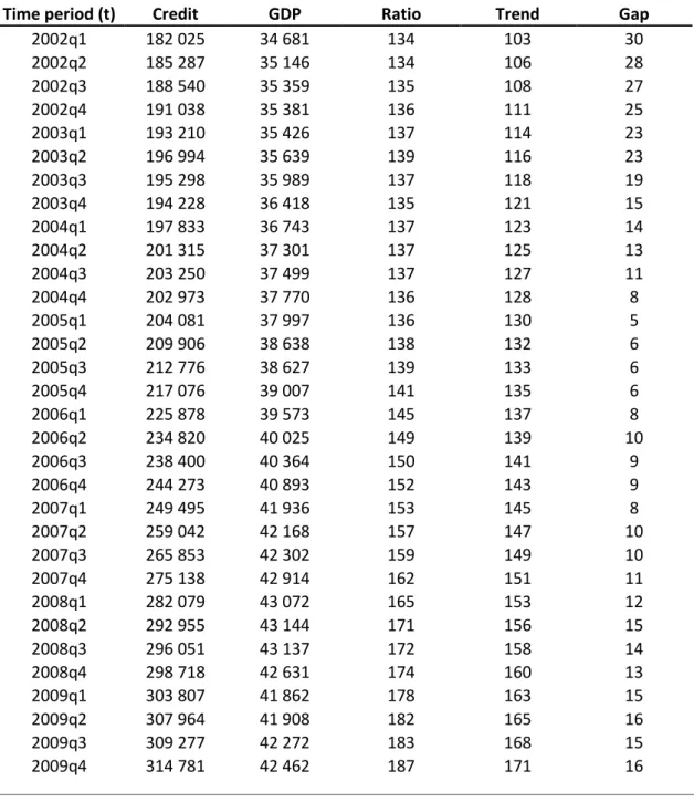
Table 6 below, presents the results of the credit-to-GDP gap in the period of 2002q1 to 2011q3, using a one sided Hodrick-Prescott filter with a smoothing parameter (λ) set to 400.000 to compute the trend.

Time period (t) Credit GDP Ratio Trend Gap

2002q1 182 025 34 681 134 103 30 2002q2 185 287 35 146 134 106 28 2002q3 188 540 35 359 135 108 27 2002q4 191 038 35 381 136 111 25 2003q1 193 210 35 426 137 114 23 2003q2 196 994 35 639 139 116 23 2003q3 195 298 35 989 137 118 19 2003q4 194 228 36 418 135 121 15 2004q1 197 833 36 743 137 123 14 2004q2 201 315 37 301 137 125 13 2004q3 203 250 37 499 137 127 11 2004q4 202 973 37 770 136 128 8 2005q1 204 081 37 997 136 130 5 2005q2 209 906 38 638 138 132 6 2005q3 212 776 38 627 139 133 6 2005q4 217 076 39 007 141 135 6 2006q1 225 878 39 573 145 137 8 2006q2 234 820 40 025 149 139 10 2006q3 238 400 40 364 150 141 9 2006q4 244 273 40 893 152 143 9 2007q1 249 495 41 936 153 145 8 2007q2 259 042 42 168 157 147 10 2007q3 265 853 42 302 159 149 10 2007q4 275 138 42 914 162 151 11 2008q1 282 079 43 072 165 153 12 2008q2 292 955 43 144 171 156 15 2008q3 296 051 43 137 172 158 14 2008q4 298 718 42 631 174 160 13 2009q1 303 807 41 862 178 163 15 2009q2 307 964 41 908 182 165 16 2009q3 309 277 42 272 183 168 15 2009q4 314 781 42 462 187 171 16

(21)

Rui Fonseca 21 2010q1 314 107 43 030 185 173 12 2010q2 319 077 42 874 187 175 12 2010q3 323 988 43 494 189 178 11 2010q4 329 618 43 273 191 180 11 2011q1 336 548 43 220 195 183 12 2011q2 335 303 42 761 194 185 9 2011q3 332 996 42 799 194 187 7

Table 6 – Credit-to-GDP gap (one-sided HP; Lambda 400 000)

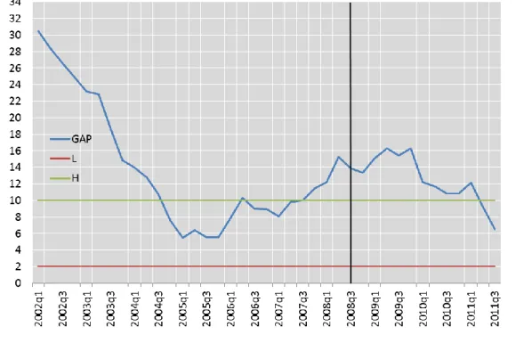
Observing the results, we can see that the gap was above the lower threshold of 2 for all periods and also that the maximum value did not occur in the 2 to 3 years’ time period preceding the crisis (see Figure 3). For these reasons, the conclusion should be that the credit-to-GDP gap using a one sided Hodrick-Prescott filter with a smoothing parameter set to 400.000 to compute the trend, did not performed as expected. One possible explanation may be the important vulnerabilities built up in the Portuguese economy in the late 90s/early 00s (e.g. strong credit growth, house prices growth, current account imbalances). Very likely, the gap was always above 2 because these vulnerabilities were never corrected, until recently.

Figure 3 – Credit-to-GDP gap (one-sided HP; Lambda 400 000)

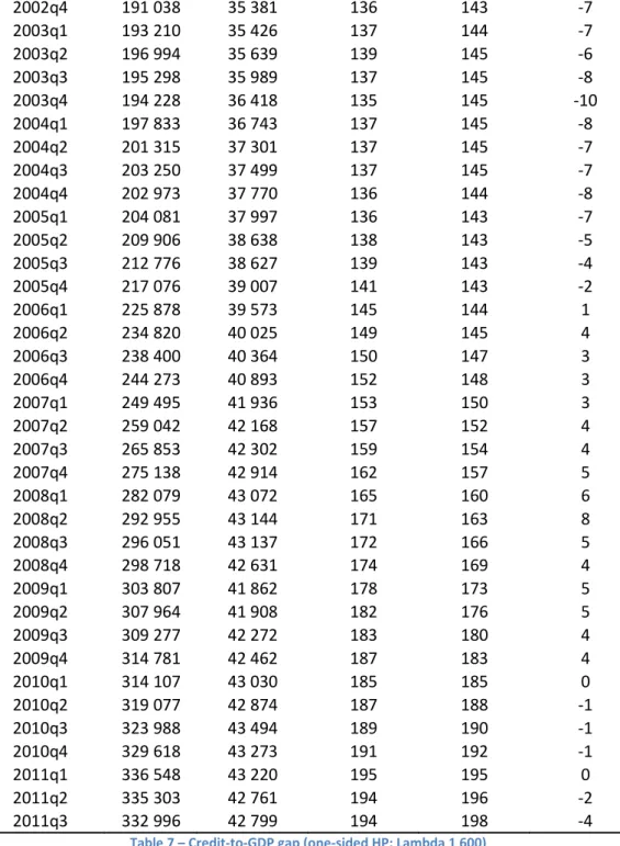
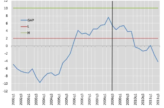
As mentioned before, the same methodology was applied using a one sided Hodrick-Prescott filter with a smoothing parameter set to 1 600 to compute the trend, as suggested by Hodrick and Prescott (1997) for quarterly data. The results are shown in the following table and figure.

Time period (t) Credit GDP Ratio Trend Gap

2002q1 182 025 34 681 134 138 -5

2002q2 185 287 35 146 134 140 -6

(22)

Rui Fonseca 22 2002q4 191 038 35 381 136 143 -7 2003q1 193 210 35 426 137 144 -7 2003q2 196 994 35 639 139 145 -6 2003q3 195 298 35 989 137 145 -8 2003q4 194 228 36 418 135 145 -10 2004q1 197 833 36 743 137 145 -8 2004q2 201 315 37 301 137 145 -7 2004q3 203 250 37 499 137 145 -7 2004q4 202 973 37 770 136 144 -8 2005q1 204 081 37 997 136 143 -7 2005q2 209 906 38 638 138 143 -5 2005q3 212 776 38 627 139 143 -4 2005q4 217 076 39 007 141 143 -2 2006q1 225 878 39 573 145 144 1 2006q2 234 820 40 025 149 145 4 2006q3 238 400 40 364 150 147 3 2006q4 244 273 40 893 152 148 3 2007q1 249 495 41 936 153 150 3 2007q2 259 042 42 168 157 152 4 2007q3 265 853 42 302 159 154 4 2007q4 275 138 42 914 162 157 5 2008q1 282 079 43 072 165 160 6 2008q2 292 955 43 144 171 163 8 2008q3 296 051 43 137 172 166 5 2008q4 298 718 42 631 174 169 4 2009q1 303 807 41 862 178 173 5 2009q2 307 964 41 908 182 176 5 2009q3 309 277 42 272 183 180 4 2009q4 314 781 42 462 187 183 4 2010q1 314 107 43 030 185 185 0 2010q2 319 077 42 874 187 188 -1 2010q3 323 988 43 494 189 190 -1 2010q4 329 618 43 273 191 192 -1 2011q1 336 548 43 220 195 195 0 2011q2 335 303 42 761 194 196 -2 2011q3 332 996 42 799 194 198 -4

(23)

Rui Fonseca 23

Figure 4 – Credit-to-GDP gap (one-sided HP; Lambda 1 600)

These results suggest that with a smoothing parameter set to 1 600 to compute the trend, the lower threshold is reached in 2006q2, which is on the period of 2 to 3 years prior to the crisis (Basel Committee on Banking Supervision, 2010). However the maximum buffer would not be reached prior to the crisis, suggesting that other thresholds should be used. Figure 5 shows an example for the lower and higher thresholds of 1 and 7, respectively.

(24)

Rui Fonseca 24 In conclusion, the gap based on the trend computed with a Hodrick-Prescott filter with a smoothing parameter set to 400 000 did not perform as expected and so it does not prove to be a perfect guide for Portugal. On the other side, the gap based on the trend computed with a Hodrick-Prescott filter with a smoothing parameter set to 1 600 delivered good results, although new thresholds may be required. For example, setting these parameters to 1 and 7 would allow the buffer to start the build up in 2006q1 and reach its maximum in 2008q2, complying with both the objectives of reaching the lower threshold at least 2 to 3 prior to the crisis and also reach the maximum buffer prior to a crisis.

4 Capital requirements: How do banks adjust?

After verifying the historical performance of the common guide credit-to-GDP, another question has to be answered in order to judge the effectiveness of the countercyclical capital buffer in Portugal: will higher capital requirements constrain credit growth?

In this chapter the aim is to address this question, using a methodology based on the previous work of Francis and Osborne (2012), which studied the effects of regulatory capital requirements on capital, lending and balance sheet management of UK banks. They concluded that raising capital requirements may be less effective in the objective of constraining credit growth if banks can comply with them by using capital of lower quality and cost.

Francis and Osborne (2012) use on the analysis capital requirements available at the UK supervisor, which include bank-specific and time-varying add-ons set in an approach similar to the one adopted by many countries under Pillar 2 of Basel II. Pillar 2, concerned with the supervisory review process, goes beyond the minimum capital requirements (Pillar 1) and allow regulators in different countries some discretion in how rules are applied, taking into account local conditions and identified deficiencies. In Portugal this data is not available and there is no evidence, based on banks' annual reports, that Pillar 2 is actively used. To replicate, to some extent, Francis and Osborne (2012) the recent changes in capital requirements for the Portuguese banking system were explored.

(25)

Rui Fonseca 25

4.1 Capital requirements: How do banks adjust? – Methodology

As mentioned before, the methodology used to find the impact of capital requirements in the balance sheet management of Portuguese banks is based on the previous work of Francis and Osborne (2012), which relies on three main steps:

1) Establish the target capital ratios of each bank;

2) Measure surplus or deficit of capital ratio to target capital ratio (capitalization index); 3) Use the capitalization index as an explanatory variable in regressions of bank balance sheet

components.

Below, are the details of each step:

1) Establish the target capital ratios of each bank

These target capital ratios depend on characteristics of each bank for the observed periods and idiosyncratic factors affecting the bank choices, and is modeled by the following formula:

∑

Equation 5 – Target capital ratio

where, is the target capital ratio of bank in period , are the characteristics of bank

in period and is a fixed effect representing the idiosyncratic factors affecting bank .

The choice of the variables representing the characteristics of banks was also based on the work of Francis and Osborne (2012). The chosen variables were:

a) (CR) Capital requirements

As mentioned before, unlike the UK where capital requirements are bank-specific and time-varying, the minimum solvency ratio in Portugal remains unchanged and equal for all banks during the observation period. However, the minimum core tier 1 ratio was set to a minimum of 9% in 2011 and 10% from 2012 and beyond (Notice 3/2011 of Bank of Portugal). In practice, setting the minimum core tier 1 ratio above the minimum solvency ratio implies that banks must have higher solvency ratios and so, this variable assumes the value of 8% for all periods except for 2011 and 2012, where it assumes the values of 9% and 10%, respectively.

(26)

Rui Fonseca 26 b) (RISK) RWA/Total Assets

This variable intends to represent the regulatory risk profile of the bank. As mentioned before, risk weighted assets are the bank’s assets and off-balance sheet exposures, weighted according to risk. The risk weight applied to each exposure must comply with the regulation set by national authorities.

c) (PROVISIONS) Provisions/Total Assets

This variable intends to represent the risk profile of the bank according to its own estimate. The economic value of each asset is its gross amount corrected by provisions that should represent the expected loss associated to the asset. Bank’s use their own models to determine this expected loss, which can be seen as proxy for risk incurred (higher levels of provision reflect a higher perception of risk).

d) (SIZE) Demeaned value of the log of total assets

This variable measures the relative size of each bank on the sample, because according to Francis and Osborne (2012), “larger banks may be better able to diversify risks,

access funding and adjust capital compared with smaller institutions.”

Francis and Osborne (2012) also included another two variables, not included in my analysis. The first was the tier 1 ratio over total capital, representing the weight of high quality capital on total capital. Because, in Portugal, the minimum core tier 1 ratio is higher than the total capital ratio this variable is not meaningful in the context.

The second variable was the ratio of trading book to total balance sheet assets, to control for several business models in institutions with great trading activity. In the case of Portuguese banks, the trading book does not have materiality compared to the banking book, so this variable was excluded.

Assuming that banks take time to adjust their capital towards the target, and again following Francis and Osborne (2012), it was considered a partial adjustment model, where the variation of the capital ratio in each period depends on the target capital ratio ( ) and the real capital

ratio of the previous period ( ). The equation is as follows:

( )

(27)

Rui Fonseca 27 where, and are the actual capital ratios of bank in the periods and ,

respectively, is the target capital ratio of bank in period , and is the error term.

Substituting Equation 5 into Equation 6 and rearranging gives the first equation of estimation:

( ) ( ∑

)

Equation 7 – Equation of estimation of capital ratio

Because Equation 7 was in fact estimated using one lag of the dependent variable and one lag of the explanatory variables, the equation is actually:

∑

Equation 8 – Equation of estimation of capital ratio using one lag of dependent and explanatory variables

where = in Equation 7, = ( ) in Equation 7 and = in Equation 7.

2) Measure surplus or deficit of capital ratio to target capital ratio (capitalization index)

After estimating the coefficients in Equation 8, the target capital ratio is computed according to Equation 5, being the long run effect of each explanatory variable given by:

Equation 9 – Long run effect of each explanatory variable

The computed target capital ratio is then used to calculate a measure of surplus or deficit of capital ratio to target capital ratio (capitalization index), according to the formula:

( )

Equation 10 – Capitalization index

where, is the capitalization index of bank in period , is the actual capital ratio of bank

(28)

Rui Fonseca 28 3) Use the capitalization index as an explanatory variable in regressions of bank balance sheet

components.

In order to pursue its target capital ratios, banks may take measures that affect the numerator of the ratio, as raising or lowering the own funds levels or they can take measures that affect the denominator of the ratio, as changing the volume of loans, leveraging or de-leveraging and by changing the risk profile of the assets.

To assess how banks in Portugal manage their balance sheets to move towards the desired capital ratio, the capitalization index (which depends on capital requirements) is used as an explanatory variable in regressions of some balance sheet and regulatory items. Following Francis and Osborne (2012), the dependent variables analyzed are the annual growth rate of loans, total assets, RWA and regulatory capital. Other explanatory variables also used in the regressions to control for other factors that may affect the dependent variables are:

a. (DProvision) Change in the ratio of provisions to assets at period

This variable is intended to control for general credit conditions (e.g. an increase of provisions represent a deterioration of the credit quality of borrowers).

b. (NPL) Ratio of non-performing loans to assets at period

This variable is intended to control for general credit conditions (e.g. an increase of non-performing loans represent a deterioration of the credit quality of borrowers).

c. (VarGDP) Annual growth of GDP

This variable is intended to control for general macroeconomic conditions.

d. (VarECBR) Annual growth of European Central Bank (ECB) refi rate This variable is intended to control for general monetary conditions.

e. (VarCPI) Annual growth of Portuguese Consumer Price Index (CPI) This variable is intended to control for general price conditions.

The next four equations reflect some of the options available to banks for responding to capital regulation and achieving their internal capital targets. Three focus on how banks adjust through altering the denominator of their capital ratios, through changing total assets (TA),

(29)

Rui Fonseca 29 risk-weighted assets (RWA), or loans (LOANS). One assesses how banks revise capital ratios by altering the numerator directly through regulatory capital (REGK).

Equation 11 – Loans regression

Equation 12 – Total assets regression

Equation 13 – RWA regression

Equation 14 – Regulatory capital regression

where, is the annual growth rate of Loans of bank in period , calculated as

( ( ) ( )), is the annual growth rate of Total assets of

bank in period , calculated as ( ( ) ( )), is the annual

growth rate of RWA of bank in period , calculated as ( ( ) ( )),

is the annual growth rate of Regulatory capital of bank in period , calculated as ( ( ) ( )), is the capitalization index of bank in period ,

is annual growth of GDP in period , is annual growth of ECB refi rate

in period , is annual growth of CPI in period , is the change in

the ratio of provisions to assets of bank in period , is the ratio of non-performing

(30)

Rui Fonseca 30

4.2 Capital requirements: How do banks adjust? – Data

On this analysis, it was used yearly data from 2000 to 2012. A long dataset is necessary given the dynamic structure of the model and the nature of the issue analyzed (balance sheet adjustments). The macroeconomic variables were obtained from Bloomberg (CPI and ECB refi rate) and Bank of Portugal (GDP). The banking data was significantly harder to obtain and constituted the biggest challenge of the entire work and was also responsible for a considerable delay on its conclusion. The objective at the beginning was to obtain quarterly data from a single source for the majority of Portuguese banks and for that objective many sources were attempted, such as SNL (could not get access), Bloomberg (does not have sufficiently long series), Bankscope (does not have sufficiently long series), Banks Almanac (only has data starting in 2007), Bank of Portugal (the publicly and available data consists only on banks annual reports since 2006), Coface (does not have banking data), InformaD&B (does not have banking data), banks’ web sites (do not contain annual reports for all periods and some of the required variables are not always available). Given the constraints, the only feasible solution was to collect annual data (consolidated level) from three different sources for the six biggest banks in the Portuguese banking system, excluding Caixa Geral de Depósitos (being a public bank, capital management does not necessarily pursue the same objectives of the remaining banking sector), which gives a sample size of 78 observations.

The three sources sorted by the priority given for collecting data were Bankscope, Bloomberg and bank’s annual reports.

Table 8 presents descriptive statistics of the variables used in Equation 8 of the first step (to establish the target capital ratios of each bank). As can be observed, banks have always held capital ratios above the minimum required, although the average gap is not considerable (about 2.7%).

Variable Observations Mean Standard deviation

Min Max Unit

CR 78 8.2308 0.5794 8.0000 10.0000 Percentage

K 78 10.9554 1.3795 8.0200 15.0000 Percentage

RISK 78 0.6856 0.0943 0.4700 0.8500 Ratio

PROVISIONS 78 0.0061 0.0048 0.0005 0.0294 Ratio

SIZE 78 0.0000 0.3260 -0.6078 0.5225 Ratio

(31)

Rui Fonseca 31 Table 9 presents the correlation matrix of the variables used in Equation 8 of the first step and the results are as expected. Being a function of RWA, RISK has a negative correlation with K, and for higher capital requirements (CR) the risk taken decreases, possibly reflecting the cost of capital. RISK has a positive correlation with PROVISIONS and SIZE, meaning that more risk is associated with higher levels of provisions and that bigger banks take more risks. CR is positively correlated with K, as it should be, and banks’ own perception of the risk taken (PROVISIONS) is correlated with higher capital ratios. The results also suggest that bigger banks tend to have higher capital ratios and lower levels of provisions.

K RISK CR PROVISIONS SIZE

K 1.0000

RISK -0.1588 1.0000

CR 0.2453 -0.2309 1.0000

PROVISIONS 0.0706 0.0081 0.5553 1.0000

SIZE 0.1757 0.0257 0.0000 -0.2472 1.0000

Table 9 – Correlation matrix of step 1 variables

Table 10, below, shows some descriptive statistics of the variables used in the regressions of the step three. The capitalization index (Z) is on average negative, which means that banks held, on average, less capital compared to the target. Z has also a disperse distribution, ranging from a minimum of -50.82% to a maximum of 38.04% and with a standard deviation of 19.94. Apart from the ECB refi rate, that on average decreased along the observation period, the rest of the variables presented a positive variation on average.

Variable Observations Mean Standard deviation

Min Max Unit

Z 72 -8.1161 19.9428 -50.8200 38.0400 Percentage VarGDP 72 0.0233 0.0280 -0.0300 0.0600 Percentage VarECBR 72 -0.3333 0.8307 -1.5000 1.2500 Percentage VarCPI 72 0.0258 0.0120 0.0000 0.0400 Percentage Dprovision 72 0.0005 0.0034 -0.0121 0.0148 Ratio NPL 72 0.0182 0.0124 0.0023 0.0569 Ratio VarlnLOANS 72 6.3022 8.0768 -13.9700 24.9800 Percentage VarlnTA 72 6.3494 7.8773 -13.8600 24.1600 Percentage VarlnRWA 72 5.2468 9.6547 -13.6700 35.3600 Percentage VarlnREGK 72 7.0186 15.3359 -30.1400 48.6300 Percentage

Table 10 – Descriptive statistics of step 3 variables

The complete series used in the regressions of step one and two are presented in Annexes 6.2 and 6.3.

(32)

Rui Fonseca 32

4.3 Capital requirements: How do banks adjust? – Results

The results of the regression using Equation 8 are shown in Table 11, below. As can be observed, not all variables are statistically significant at the 10% level. RISK has a p-value of 0.19 and PROVISIONS has a p-value of 0.12, slightly above the threshold of 0.10. The most statistically significant variables were K with a p-value of 0.01 and CR with 0.03. It is important for the analysis the significance of CR and the coefficient estimated, which means that capital requirements are an important driver for capital ratios.

Variable Coefficient Kt-1 0.335** (0.127) CRt-1 1.735** (0.760) RISKt-1 3.679 (2.805) PROVISIONSt-1 72.75 (46.38) SIZEt-1 -8.447* (5.041) -0.024 (0.446) 2.792 (1.744) 1.650* (0.963) 0.0244 (0.446) -6.229** (3.088) -3.188 (2.064) Constant -8.741 (6.445) Observations 72 R-squared 0.411

Robust standard errors in parentheses *** p<0.01, ** p<0.05, * p<0.1

Table 11 – Results of the regression using Equation 8 (dependent variable: kt)

As explained before, in the second step Z is computed using Equation 5, Equation 9 and Equation 10. Because some of the bank variables did not present statistically significance at

(33)

Rui Fonseca 33 the 10% level (Table 11),they were excluded from the calculation of the target capital ratio (e.g. RISK and PROVISIONS).

The results presented in Table 12 were obtained using the computed Z as an input for the regressions using Equations 11 to 14 and also the rest of the explanatory variables already mentioned (VarGDP, VarECBR, VarCPI, DProvision and NPL). Although there is a positive association between the capitalization index (Z) and the variation of Loans, Total assets and RWA, the results do not present the necessary significance to take liable conclusions. On the other side there is a significantly negative association between the level of capitalization (Z) and regulatory capital, which seems to suggest that Portuguese banks tend to react to the raising of capital requirements by changing the numerator of the ratio. These finding are consistent with the capital increases that most banks did on the recent past (some of them with funds stemming from the Portuguese government). However, it is important to remember that capital requirements increased in Portugal during a crisis period, and further, the objective was not to act countercyclically, as clearly there was not a credit boom building up.

Another negative and statistically significant association is observed between the variation of provisions and the variation of Loans, Total assets and RWA, suggesting that an increase in provisions (risk taken assessed by the bank) is associated with de-leveraging and the lowering of the risk profile. In fact, de-leveraging in the Portuguese economy is being driven by the increase in credit risk in the economy, which is forcing the banks to record more provisions and is thereby exerting strong pressure on profitability.

In sum, tighter capital requirements seem to be addressed by banks through increases in capital rather than through de-leveraging. Although these results might imply that imposing an additional capital buffer will lead to additional capital increases, the fact that in Portugal capital requirements were increased pro-cyclically indicates that these results cannot be generalized and does not allow to conclude that increases of capital requirements during a credit boom due to the build up of the countercyclical buffer will necessarily lead to the same adjustment by banks. Nevertheless, given the lack of empirical evidence on this very important issue, I hope that these results help to shed some light on the possible adjustments made by banks following an increase in capital requirements.

(34)

Rui Fonseca 34

Variable VarLnLoans VarLnTA VarLnRWA VarLnRegK

Z 0.0232 0.0618 0.0649 -0.666** (0.0386) (0.0615) (0.116) (0.249) VarGDP 48.73 27.81 107.6 138.3 (37.16) (23.82) (59.22) (77.68) VarEcbR 1.707*** 1.767** 2.250 -2.248 (0.416) (0.574) (1.474) (1.267) DProvision -1,032*** -715.6*** -1,085*** -1,828** (140.3) (138.1) (268.2) (540.3) NPL -157.0 -101.4 -66.55 -310.2 (82.86) (99.31) (130.0) (339.8) Constant 8.723*** 8.323** 5.018 4.627 (2.163) (2.233) (3.197) (7.277) Observations 66 66 66 66 R-squared 0.454 0.315 0.447 0.299 Number of ID 6 6 6 6

Robust standard errors in parentheses *** p<0.01, ** p<0.05, * p<0.1

Table 12 – Results of the regressions using Equations 11 to 14

5 Conclusions

The main objective of this thesis is to assess if the implementation in Portugal of the countercyclical capital buffer present on the Basel III framework will have the desired effect of constraining excessive credit growth in good periods of the business cycle and allow to build the necessary capital buffers to be released in crisis, thus mitigating the possibility of credit crunches.

The main objective was in practice divided in two smaller ones. The first one was to verify the historical performance of the common guide Credit-to-GDP gap proposed by the BCBS to signal the build up of the countercyclical capital buffer. The results showed that the guide can signal the build up of the buffer complying with the objectives of reaching the lower threshold at least 2 to 3 years prior to a crisis and also reach the maximum buffer prior to a crisis. However, some alterations to the methodology proposed may allow to improve the results. For instance, using a smoothing parameter set to 1 600 instead of 400 000 to compute the trend using a Hodrick-Prescott filter and changing the lower and upper thresholds to 1 and 7 may provide more useful signals to policy makers.

(35)

Rui Fonseca 35 The second objective was to assess if Portuguese banks would respond to an increase of capital requirements by contracting loan supply or by other means. To do so, it was used an approach based on the previous work of Francis and Osborne (2012), which studied the effects of regulatory capital requirements on capital, lending and balance sheet management of UK banks. The results suggest that Portuguese banks tend to react to capital requirement increases by raising the levels of regulatory capital. However, it should be borne in mind that capital requirements were increased during a crisis period (i.e. not with countercyclical objectives). As such, though this analysis hopefully provides unique evidence on how banks adjust capital, the results could only be fully generalized if more changes in capital requirements were observed. Nevertheless, given the lack of international evidence on the effects of macroprudential measures (and of the countercyclical capital buffer in particular), with this thesis I hope to provide important insights to bankers and policy-makers.

(36)

Rui Fonseca 36

6 Annexes

6.1 Quarterly data of nominal credit and nominal GDP (values in m€)

Time period (t) Credit GDP Ratio

1979q4 4 240 1 780 - 1980q1 4 520 1 867 - 1980q2 4 722 1 996 - 1980q3 4 929 2 076 64 1980q4 5 386 2 149 67 1981q1 5 749 2 298 67 1981q2 6 125 2 324 69 1981q3 6 408 2 520 69 1981q4 6 792 2 644 69 1982q1 7 128 2 749 70 1982q2 7 513 2 855 70 1982q3 7 937 3 022 70 1982q4 8 535 3 195 72 1983q1 8 891 3 454 71 1983q2 9 369 3 667 70 1983q3 9 835 3 906 69 1983q4 10 743 4 115 71 1984q1 11 058 4 264 69 1984q2 11 634 4 550 69 1984q3 12 316 4 791 70 1984q4 13 045 5 032 70 1985q1 13 277 5 320 67 1985q2 13 727 5 591 66 1985q3 13 906 5 810 64 1985q4 14 406 6 057 63 1986q1 14 607 6 329 61 1986q2 14 959 6 789 60 1986q3 15 383 7 078 59 1986q4 16 206 7 336 59 1987q1 16 627 7 574 58 1987q2 16 863 7 976 56 1987q3 17 135 8 203 55 1987q4 17 687 8 522 55 1988q1 18 347 9 111 54 1988q2 18 857 9 430 53 1988q3 19 452 9 831 53 1988q4 20 294 10 444 52 1989q1 20 191 10 680 50 1989q2 20 691 11 158 49 1989q3 21 330 11 678 49 1989q4 22 758 12287 50 1990q1 23 183 12 737 48

(37)

Rui Fonseca 37 1990q2 24 580 13 611 49 1990q3 24 420 13 947 46 1990q4 26 119 14 400 48 1991q1 27 738 14856 49 1991q2 29 476 15 523 50 1991q3 30 694 16 030 50 1991q4 33 189 16 520 53 1992q1 33 477 17 224 51 1992q2 35 326 17 814 52 1992q3 36 954 18 047 53 1992q4 39 516 18 283 55 1993q1 40 223 18 063 56 1993q2 42 114 18 415 58 1993q3 42 563 18 809 58 1993q4 44 433 19 126 60 1994q1 44 814 19 592 59 1994q2 45 982 20 141 59 1994q3 46 261 20 361 58 1994q4 49 356 20 842 61 1995q1 52 473 21 545 63 1995q2 54 833 21 899 65 1995q3 55 702 22 071 65 1995q4 58 088 22 326 66 1996q1 58 479 22 634 66 1996q2 61 561 23 100 68 1996q3 63 545 23 704 69 1996q4 67 996 23 778 73 1997q1 70 210 24 473 74 1997q2 74 056 25 114 76 1997q3 77 652 25 626 78 1997q4 82 168 25 934 81 1998q1 84 678 26 590 82 1998q2 90 923 27 395 86 1998q3 95 373 27 978 88 1998q4 102 736 28 414 93 1999q1 108 309 28 969 96 1999q2 115 140 29 403 100 1999q3 122 117 29 931 105 1999q4 129 577 30 358 109 2000q1 136 601 31 069 113 2000q2 147 115 31 369 120 2000q3 155 686 32 295 124 2000q4 160783 32 584 126 2001q1 167 915 32 815 130 2001q2 173 421 33 393 132 2001q3 177 305 33 768 134 2001q4 179 401 34 496 133 2002q1 182 025 34 681 134

(38)

Rui Fonseca 38 2002q2 185 287 35 146 134 2002q3 188 540 35 359 135 2002q4 191 038 35 381 136 2003q1 193 210 35 426 137 2003q2 196 994 35 639 139 2003q3 195 298 35 989 137 2003q4 194 228 36 418 135 2004q1 197 833 36 743 137 2004q2 201 315 37 301 137 2004q3 203 250 37 499 137 2004q4 202 973 37 770 136 2005q1 204 081 37 997 136 2005q2 209 906 38 638 138 2005q3 212 776 38 627 139 2005q4 217 076 39 007 141 2006q1 225 878 39 573 145 2006q2 234 820 40 025 149 2006q3 238 400 40 364 150 2006q4 244 273 40 893 152 2007q1 249 495 41 936 153 2007q2 259 042 42 168 157 2007q3 265 853 42 302 159 2007q4 275 138 42 914 162 2008q1 282 079 43 072 165 2008q2 292 955 43 144 171 2008q3 296 051 43 137 172 2008q4 298 718 42 631 174 2009q1 303 807 41 862 178 2009q2 307 964 41 908 182 2009q3 309 277 42 272 183 2009q4 314 781 42 462 187 2010q1 314 107 43 030 185 2010q2 319 077 42 874 187 2010q3 323 988 43 494 189 2010q4 329 618 43 273 191 2011q1 336 548 43 220 195 2011q2 335 303 42 761 194 2011q3 332 996 42 799 194