RESIST: an intelligent system to predict antibiotic resistance

UNIVERSIDADE DE LISBOA

Faculdade de Ciências

Departamento de Informática

RESIST: AN INTELLIGENT SYSTEM TO

PREDICT ANTIBIOTIC RESISTANCE

João Miguel Campos do Nascimento

DISSERTAÇÃO

MESTRADO EM ENGENHARIA INFORMÁTICA

Especialização em Sistemas de Informação

Trabalho orientado pela Prof. Doutora Cátia Luísa Santana Calisto Pesquita

UNIVERSIDADE DE LISBOA

Faculdade de Ciências

Departamento de Informática

RESIST: AN INTELLIGENT SYSTEM TO

PREDICT ANTIBIOTIC RESISTANCE

João Miguel Campos do Nascimento

DISSERTAÇÃO

MESTRADO EM ENGENHARIA INFORMÁTICA

Especialização em Sistemas de Informação

Trabalho orientado pela Prof. Doutora Cátia Luísa Santana Calisto Pesquita

Acknowledgements

First, I would like to thank my advisor, Prof. Cátia Pesquita, for her guidance, patience and all the valuable advice she constantly gave me throughout the project. It was a real pleasure to work with such a talented and supportive advisor. I am also grateful to the BIOFIG Lab at FCUL for sharing the dataset that supported this project.

The rest of the acknowledgments will be written in my mother tongue, Portuguese, so that everyone I want to thank can fully understand my gratitude.

Tenho que agradecer a toda a minha família, por todo o seu apoio constante, em especial aos meus pais, João e Hermínia, por tudo o que me deram e fizeram por mim. Pela educação que me deram, pela exigência saudável a que me habituaram e pelo financiamento de todo o meu percurso académico, estar-lhes-ei eternamente grato.

Quero ainda agradecer a todos aqueles que de alguma forma me apoiaram ao longo desta caminhada, fosse dando auxílio, fazendo trabalhos em grupo, ou simplesmente fazendo companhia e distraindo-me. Não irei discriminar nomes, pois sei que, felizmente, o tamanho da lista rivalizaria com o do resto da dissertação, e mesmo assim tenho a certeza que me faltaria sempre alguém, algo pelo qual não me perdoaria.

Quer seja alguém do Infantado, de Loures, da FCUL ou de outro sítio qualquer, qualquer pessoa com quem eu tenha tido o prazer de falar, pessoalmente ou mesmo apenas virtualmente, e me tenha apoiado, mesmo que não o saiba, tem a minha gratidão. Tenho ainda que agradecer a duas das maiores paixões da minha vida, o Infantado Futebol Clube e o Sporting Clube de Portugal, que, ainda que não sejam pessoas, me servem de escapatória para o mundo real e me permitem temporariamente limpar a cabeça de todos os problemas.

Finalmente, quero deixar uma palavra de agradecimento àqueles que já partiram. Aos meus avós, José, Constantino e Odete, que sei o quão orgulhosos estariam de mim se ainda cá estivessem, e aos meus companheiros de quatro patas, King e Batata, os irmãos que nunca tive, que comigo partilharam e alegraram os meus dias de infância e adolescência, respectivamente. A todos eles o meu obrigado, carregado de saudades.

i

Resumo

Os recentes avanços na tecnologia e poder computacional e o cada vez mais frequente uso de registos de saúde eletrónicos abriram as portas a novas pesquisas que exploram a informação destes registos para melhorar os cuidados médicos, nomeadamente nos diagnósticos e nas prescrições terapêuticas.

Uma das maiores preocupações em termos de saúdes pública é a resistência a antibióticos. Este fenómeno ocorre quando algumas das subpopulações de um microrganismo sobrevivem após serem expostas a antibióticos, tornando-se mais difíceis de controlar. É, portanto, essencial utilizar antibióticos de uma forma mais eficaz. A Organização Mundial de Saúde já declarou publicamente que, a não ser que se consiga reduzir o rápido crescimento da resistência a antibióticos a que tem assistido, estamos a caminhar para uma era pós-antibióticos, onde a taxa de mortalidade por infeções comuns vai disparar devido à falha expectável de tratamentos médicos habituais.

Hoje em dia, o antibiótico mais adequado apenas pode ser descoberto após os resultados dos testes dos laboratórios de análise serem conhecidos, então a maioria dos médicos fazem prescrições com base na sua experiência. No entanto, ao analisar um grande volume de dados clínicos, é possível que o pessoal clínico descubra informações mais relevantes que podem ajudá-los nas suas decisões. A equipe médica deve ter mais informações aquando da tomada de decisões.

A análise computacional dos registos de saúde electrónicos representa uma oportunidade para combater a tendência crescente de resistência aos antibióticos, pois a nova informação descoberta pode auxiliar os médicos na tomada de melhores diagnósticos e prescrições. Isso poderia aumentar a qualidade da assistência médica, reduzindo não só a mortalidade e morbidade, mas também os custos.

O objetivo deste projeto foi investigar se era possível desenvolver modelos de aprendizagem supervisionadas que fossem capazes de classificar os pacientes consoante

ii

o risco de resistência a antibióticos utilizando as informações que são geralmente recolhidas a nível clínico e laboratorial em termos de resistência aos antibióticos. O conjunto de dados que apoiaram este projecto foi gentilmente partilhado através de uma colaboração com o Laboratório de BIOFIG na FCUL, e representa dados reportados por vários hospitais portugueses em matéria de resistência aos antibióticos durante um período de 11 anos.

Duas tarefas foram realizadas para cumprir os objectivos: pré-processamento dos dados e aprendizagem supervisionada. No pré-processamento dos dados foram usadas técnicas de limpeza, de estandardização e de transformação de dados, de modo a tornar os dados o mais consistente possível para que pudessem depois seguir para a aprendizagem supervisionada. Aqui foram aplicados métodos de aprendizagem automática sobre os dados para treinar um modelo capaz de prever a resistência aos antibióticos ao nível do paciente, com base em parâmetros demográficos, clínicos e laboratoriais.

Numa primeira fase, a classificação de cada paciente como resistente ou não resistente a cada antibiótico foi realizada individualmente. Nela foram testados diversos algoritmos, como Decision Tables (DT), Random Forests (RF), Multilayer Perceptron (MP) e Support Vector Machines (SVM), sempre com validação cruzada com 10 subconjuntos. Foram ainda feitos testes com os filtros SMOTE a 200% e 500% e Spread Subsample com um rácio 1:1.

Os resultados não foram satisfatórios, portanto os testes foram repetidos após se fazer uma avaliação sobre ganho de informação dos atributos, de modo se testar apenas sobre os atributos mais relevantes. No entanto, os resultados pouco melhoraram.

Foi então compreendido que a formulação inicial do problema (uma classe para cada antibiótico) era provavelmente inadequada. Assim sendo, problema de classificação foi reformulado, desta feita seguindo para uma abordagem de classificação por perfil de resistência dos pacientes. Técnicas de agrupamento foram aplicadas sobre os dados para identificar perfis de resistência, ou seja, pacientes que apresentaram resistência ao mesmo conjunto de antibióticos.

Após isso, uma estratégia de classificação de dois níveis foi concebida de forma a classificar os pacientes de acordo com o seu perfil de resistência.

Para o primeira nível, a classificação filtrada, uma estratégia de classificação duas classes foi utilizada, em que todas as instâncias pertencentes a grupos de perfis

iii

resistentes foram agrupados numa única classe, enquanto que os restantes doentes sem qualquer resistência foram agrupados noutra classe distinta. A classificação filtrada foi sempre realizada com um filtro SMOTE com a percentagem a 500% e os algoritmos de classificação foram testados Decision Tables e Random Forests, com uma validação cruzada com 10 subconjuntos.

Seguidamente, no segundo nível, as instâncias que foram classificadas como resistentes foram novamente separadas consoante os resultados da técnica de agrupamento anteriormente utilizada, classificadas via classificação multi-classe, para que o conjunto de dados multi-classe pudesse ser tratado por classificadores de 2 classes. Os algoritmos de classificação utilizados foram os mesmos que para o primeiro nível, apenas sem filtro, e os métodos utilizados para transformar o problema multi-classe em vários de 2 multi-classes foram 1-contra-todos e 1-contra-1.

Notou-se uma melhoria geral nos resultados, mas ainda com um desempenho bastante reduzido na maioria dos perfis. Outras duas abordagens foram feitas usando esta estratégia de classificação de dois níveis. Uma baseada numa classificação direta de instâncias em perfis de resistência, corrigindo algumas das atribuições erradas dos agrupamentos feitas pelo algoritmo de agrupamento, tendo as instâncias que foram erradamente colocadas num agrupamento sido realocadas. A outra, para além do reajustamento que acabou de ser explicado, continha ainda o número de instâncias pertencentes a cada agrupamento por mês. Novamente, apesar de terem sido notadas melhoras gerais, não eram suficientemente satisfatórias. Foram ainda realizadas previsões futuras sobre a evolução futura do número de pacientes resistentes por perfil de resistência recorrendo a séries temporais.

Apesar dos resultados da classificação por perfil de resistência terem um baixo desempenho no geral, tiveram algum sucesso com o perfil onde os pacientes eram resistentes a Tetramicina e Cloranfenicol. Dadas as várias falhas detectadas a nível da qualidade dos dados (dados em falta, heterogeneidade de nomeações e categorias, número reduzido de pacientes resistentes para alguns antibióticos) é expectável que o desempenho para outros perfis possa aumentar, utilizando um conjunto de dados com maior qualidade e representatividade.

Este projecto realçou dois aspectos importantes: a qualidade e representatividade dos dados recolhidos, pois após terem sido testadas várias abordagens diferentes e os resultados correspondentes analisados, foi determinado que a informação reportada não

iv

tinha a capacidade preditiva apropriada, pelo que não foi possível desenvolver o modelo anteriormente descrito; e a compreensão dos dados e do seu domínio, verificado quando se demonstrou que a classificação por perfil de resistência obteve melhores resultados que a classificação por antibiótico.

Uma vez que os dados recolhidos cobrem um período de até há 10 anos, é expectável que com as recentes evoluções nos sistemas de informação de saúde empregues por hospitais portugueses, uma recolha de dados mais recentes iria fornecer dados de melhor qualidade. Seria assim interessante aplicar a estratégia proposta sobre dados mais recentes, e testar estes iriam de facto melhorar o desempenho da classificação.

Palavras-chave: Aprendizagem supervisionada, aprendizagem automática sobre dados

clínicos, previsão de resistência a antibióticos, prospeção de dados, registos de saúde eletrónicos

v

Abstract

The recent advances in technology and computation power and the expanding use of electronic health records have opened new avenues of research that explore the information in these records to improve healthcare, namely in diagnosis and therapeutic prescriptions. One increasingly relevant public health concern is antibiotic resistance. The World Health Organization has already stated that unless the antibiotic resistance's growing trend is reduced, we are heading towards a post-antibiotic era, where the death rate of common infection will rise due to the expected failure of standard medical treatments.

The ability to successfully predict antibiotic resistance risk can have a significant impact worldwide, because it can help clinicians in selecting appropriate antibiotics. This can help reduce antibiotic resistance levels, improve patient treatment, and ultimately decrease healthcare costs.

This project's goal is to investigate if it is possible to develop supervised learning models that are able to classify patients regarding their antibiotic resistance risk using the information that has been usually collected at a clinical and laboratorial level and reported by Portuguese hospitals. This was accomplished by taking electronic health records data, pre-processing it using data cleaning, standardization and transformation techniques, and then applying machine learning methods to it to train a model capable of predicting antibiotic resistance at the patient level.

The most successful classification strategy was based on a two-stage multi-class approach, where patients were classified into resistance profiles previously obtained using clustering techniques. Nevertheless, performance was still very low for most resistance profiles, no doubt influenced by the several issues in data quality detected. An improved collection of data, with fewer errors and other variables reported would likely have a great impact in performance.

vi

Keywords: Supervised learning, machine learning on clinical data, antibiotic resistance

vii

Contents

Chapter 2 State of the Art ... 5

2.1 Basic concepts ... 5

2.2 Related work ... 7

Chapter 3 Methods ... 11

3.1 Data Characterization ... 11

3.2 Data Cleaning and Normalization ... 13

3.3 Data Transformation ... 13

3.4 Classification by Antibiotic ... 14

3.5 Antibiotic Resistance Profiling ... 16

3.6 Classification by Resistance Profile ... 16

3.7 Time Series ... 19

Chapter 4 Results ... 21

4.1 Data Normalization and Transformation ... 21

4.2 Statistical Analysis ... 23

4.3 Classification by Antibiotic ... 24

4.4 Antibiotic Resistance Profiling ... 30

4.5 Classification by Profile Resistance ... 31

4.6 Time Series ... 35

Chapter 5 Discussion ... 39

Chapter 6 Conclusions ... 43

Bibliography ... 45

Appendices ... 49

Appendix I: Parameters used for each classification algorithm ... 49

Appendix II: Classification by profile resistance results for patients whose test fluid was cerebrospinal fluid ... 51

ix

List of Figures

Figure 3.3.1: NUTS II Regions of Portugal ... 14

Figure 3.6.1: Two-stage classification strategy architecture ... 17

Figure 4.2.1: Resistant patients by antibiotic ... 24

Figure 4.4.1: Clustered instances by cluster... 31

Figure 4.5.1: Clustered instances by cluster after cluster adjustment ... 33

Figure 4.6.1: One-step-ahead predictions for cluster 7 ... 36

Figure 4.6.2: Future forecast for cluster 7 ... 36

Figure 4.6.3: One-step-ahead predictions for cluster 9 ... 37

xi

List of Tables

Table 3.1.1: Main features of the dataset ... 12

Table 4.1.1: Data normalization examples ... 21

Table 4.1.2: Data transformation examples ... 22

Table 4.2.1: Number of blank entries in each relevant feature ... 23

Table 4.3.1: Classification by antibiotic results using Decision Tables ... 25

Table 4.3.2: Classification results for Tetramycin using other algorithms ... 25

Table 4.3.3: Classification by antibiotic results using Decision Tables with a SMOTE filter (200%) ... 26

Table 4.3.4: Classification results for Tetramycin using other algorithms with a SMOTE filter (200%) ... 26

Table 4.3.5: Classification by antibiotic results using Decision Tables with a Spread Subsample filter ... 27

Table 4.3.6: Classification results for Tetramycin using other algorithms with a Spread Subsample filter ... 27

Table 4.3.7: Classification by antibiotic results using Decision Tables with a SMOTE filter (500%) ... 28

Table 4.3.8: Classification results for Tetramycin using other algorithms with a SMOTE filter (500%) ... 28

Table 4.3.9: Classification results for Tetramycin using feature selection ... 29

Table 4.3.10: Classification results for antibiotic families using Decision Tables 29 Table 4.4.1: Relation between clusters and resistance profiles ... 30

Table 4.5.1: Classification results for the first step of the two-stage classification strategy without cluster adjustment ... 31

Table 4.5.2: Classification results for the second step of the two-stage classification strategy without cluster adjustment ... 32

Table 4.5.3: Classification results for the first step of the two-stage classification strategy with cluster adjustment ... 33

Table 4.5.4: Classification results for the second step of the two-stage classification strategy with cluster adjustment ... 34

xii

Table 4.5.5: Classification results for the first step of the two-stage classification strategy with month values ... 34

Table 4.5.6: Classification results for the second step of the two-stage classification strategy with month values ... 35

Table 4.6.1: mean absolute error values for one-step-ahead predictions ... 38

1

Chapter 1

Introduction

This dissertation is focused on predicting antibiotic resistance risk for patients using supervised learning approaches over demographic, clinical and laboratory data. The first chapter will present my motivation, objectives and contributions, as well as the document structure.

1.1 Motivation

Antibiotic resistance is one of the public healthcare’s main concerns, mainly for driving up healthcare costs, increasing the severity of disease, and increasing the death rates of some infections [1-3]. The WHO’s (World Health Organization) 2014 report on global surveillance of antimicrobial resistance [4] shows that antibiotic resistance is an actual problem at a global scale, putting at risk the ability to treat common infections in the community and hospitals.

Nowadays, the most appropriate antibiotic can only be found after the lab analysis test results are known, so most of the doctors make prescriptions based on their experience alone. It is vital to use antibiotics in a more effective way and to reduce the antibiotics resistance growing trend, or else we are headed towards a post-antibiotic era, in which common infections and minor injuries can once again kill.

The recent advances in technology and computation power, combined with the expanding use of electronic health records, represent an opportunity to fight the rising antibiotic resistance trend by aiding clinicians in making better diagnostics and therapeutic prescriptions [5]. By analyzing a large volume of clinical data, it is possible to give clinical staff more relevant information that can help them on their decisions.

2

This could potentially increase the quality of healthcare, reducing mortality and morbidity, while also reducing costs.

1.2 Objectives

This dissertation's goal was to investigate if it was possible to develop supervised learning models that were able to classify patients regarding their antibiotic resistance risk using the information that is usually collected at a clinical and laboratorial level in terms of antibiotic resistance by Portuguese hospitals. The dataset that supported this project has been kindly shared through a collaboration with the BIOFIG Lab at FCUL, and represents data reported by several Portuguese hospitals concerning antibiotic resistance over an 11 year period.

Two tasks were planned to accomplish the goal:

1. Data pre-processing: (1) Data cleaning for handling missing and corrupted values; (2) Data transformation for improved grouping of some data, such as age and antibiotic type; (3) Data standardization for solving the heterogeneities in names and scales.

2. Supervised learning: Application of machine learning methods to the data to train a model capable of predicting antibiotic resistance at the patient level, based on demographical, clinical and laboratory parameters.

1.3 Contributions

The contributions of this project include:

 The identification and solution of the data quality issues: Several problems were detected including a large portion of missing values, lack of standardized nomenclature and the usage of different scales or categories. The magnitude of these issues demonstrates that there is a need to revise

3

the EHR data collection procedure that was employed to generate the dataset.

 The creation of patient resistance profiles by clustering of individual antibiotic resistance status for each patient: These profiles allow for a better understanding of the domain, and highlight the complexity of the antibiotic resistance phenomenon.

 The development of a two-stage multi-class classification strategy to classify patients according to their antibiotic resistance profile: Although performance was very low for most of the profiles, the promising values achieved in predicting one of the profiles support further investment in this strategy using datasets with improved quality and representativity.

 This project was featured on the 4th Bioinformatics Open Days 2015 held in the Faculty of Sciences of the University of Lisbon on April 2015 in the form of a poster presentation [6].

1.4 Document structure

The document is organized in the following way:

 Chapter 2 - State of the Art: Describes some basic concepts useful for a good understanding of the project and presents some of the most of the most relevant work in the area.

 Chapter 3 - Methods: Presents the dataset and describes the methods and strategies employed along the project.

 Chapter 4 - Results: Presents a statistical analysis of the dataset, as well as the results of the classification tests described in the previous section.

 Chapter 5 - Discussion: Presents a critical discussion of the developed work, debating the fulfilment of the objective and the additional contributions.

4

 Chapter 6 - Conclusions: This section summarizes the main conclusions of this work and discusses possible avenues for future work.

5

Chapter 2

State of the Art

In this chapter some basic concepts that are crucial for a good understanding of this dissertation will be presented, including electronic health records, data mining, machine learning and time series analysis. This section is followed by relevant related work. Although supervised learning over electronic health records has been used in several clinical domains, such as oncology diagnosis [7], this review will only focus on antibiotic resistance prediction.

2.1 Basic concepts

Electronic health records (EHR) store and integrate important data, including demographic patient information, drug prescription data or medical notes describing medical reasoning behind the prescription, over time. Thanks to its administrative data, EHR is widely used in population-based health research [8]. When dealing with a certain case, doctors can study what were their peers' opinions at the time and how they affected their patients' health just by looking at data stored from previous similar cases. Furthermore, it gives doctors the ability to predict how the patient's condition will evolve, allowing them to intervene earlier [5, 9].

Data cleaning (also called data cleansing) consists of exploring the data for possible problems and making an effort to correct errors, by detecting and deleting/correcting erroneous or irrelevant records from a dataset. The quality of data used for data mining or machine learning can have a considerable impact on the performance of these strategies. There are several problems that can be found in electronic health records data, from missing, ambiguous or incorrect values to

6

misspelling errors. Therefore, data cleaning frequently involves human judgment to decide which points are valid and which are not [10].

The term dataset usually refers to data selected and arranged in rows and columns, all related but separate elements, ready to be processed and manipulated as a whole by a computer. The values in a dataset may be of any of the kinds described as a level of measurement, usually numbers or nominal data.

Data Mining techniques can be applied to EHR to discover novel insights about diseases, such as co-morbidities, patient susceptibilities, etc. Data Mining deals with large amounts of data in order to discover useful patterns or relationships unknown until the time, and is more successful if there is much data available. By making use of these large clinical data collections, it is possible to make a retrospective analysis, which brings forth an opportunity to deepen our knowledge regarding clinical processes [11, 12]. One data mining technique employed to support future predictions is time series analysis. Time series are a set of repeated observations of the same variable for statistical analysis, pattern recognition or forecasting, among other areas [13].

Machine learning algorithms provide computers with the ability to learn from data automatically without human intervention. It plays a vital role in bioinformatics and medical diagnosis nowadays [14, 15]. It is a class of algorithms that are data-driven, i.e. it is the data that dictates the best answer. Machine learning focuses on the development of computer programs that can teach themselves to grow and change when exposed to new data and deals with the construction and study of algorithms that can learn from that same data. The machine learning task inferring a function from labelled data is called supervised learning.

Machine learning is often confused with data mining, due to their significant overlap. But while machine learning acts based on the known properties from the training data, data mining is more focused on knowledge discovery (the discovery of previously unknown properties in the data). By applying machine learning techniques to the data stored in electronic medical records and electronic health records it is possible to aid diagnosis and improve therapeutic choice [5].

One kind of machine learning algorithms called supervised learning, rely on using example inputs and their desired outputs, so that the algorithm can generate a model that maps inputs to outputs. This usually means that a set of instances is classified into one of two classes according to a model learned from a number of labelled examples.

7

When datasets have more than two classes, multiclass classification is applied, which is the problem of constructing a function which, knowing that each training point belongs to one of several different classes, given a new data point, will correctly predict the class to which the new point belongs [16].

When examples are not labelled, we have unsupervised learning instead. A commonly used unsupervised learning technique is clustering. Jain et al. [17] define clustering as the unsupervised classification of patterns into groups of similar objects. Those groups are named clusters. Clustering is useful in several situations, such as pattern classification, like classifying pathologies by their features.

To improve the quality of machine learning strategies it is common to employ feature selection, the process of selecting a subset of relevant features from the data for application of a learning algorithm. When using a feature selection technique, it is assumed that the data contains irrelevant facts. The best subset contains the least number of dimensions that most contribute to accuracy, discarding those that are irrelevant. There are several feature selection techniques. One of them, related to the so-called filter approach, assumes evaluation of individual features or feature subsets independently from the learning algorithm. The wrapper approach is another technique, which assumes evaluation of feature subsets according to the accuracy of predictive model built on these feature subsets [2].

2.2 Related work

The key to controlling the spread of antibiotic resistance is using antibiotics in a smart, thoughtful way. And to do so, being able to predict a bacteria’s resistance to a given antibiotic is fundamental. Hence the extreme importance of applying data mining techniques and machine learning methods to clinical data. Several approaches have been used so far to tackle this issue. One is to take clinical data with record of ill patients and their medication, analyze their evolution, and, by crossing data to find similar cases, define what would be the best course of treatment and predict what should happen.

Pechenizkiy et al. [2] followed this approach when in 2005 they applied various data mining techniques to hospital data from patients who had meningitis for the sake of predicting antibiotic resistance for nosocomial infections. Naive Bayes, Bayesian Network, C4.5 decision trees, k-nearest (1, 3 and 15) neighbours and JRip were applied

8

as basic classifiers. The nearest neighbour-based (especially 1NN and 15NN) and the decision tree classifiers achieved the best accuracy results, all of them over 78%. On the other hand, the Bayesian features performed poorly. This may be due to the redundancy and high correlation of the features, seeing as they were all used.

However, when feature selection was applied the results differed and more relevant conclusions could be made. The filter approach usage taught them that most information was concentrated in the features related to antibiotics themselves, while the wrapper approach showed that the multidimensionality of the original space had a negative effect. Furthermore, by applying a regular manual feature selection they discovered that groupings of antibiotics and pathogens into categories were appropriate and the grouping features contained relevant information and that their data contained some interesting patterns independent from antibiotics and pathogens related to the demographics and hospital stay information only. It was safe to make these assumptions because, although the accuracy results were lower than when they had tested without feature selection, they were still much higher than 50%.

When natural clustering (strategy of grouping objects into groups of similar objects) was applied and the base classifiers were applied on the antibiotic group, who had three subgroups, it was not only observed that for two of them the cluster classifiers outperformed the global classifiers for every type of base classifiers, but also that their average accuracy is higher when they are applied locally within each cluster comparing to the global classifiers' accuracy.

Also in 2005, Tsymbal et al. [18] proposed the use of an ensemble integration technique that would help to better handle concept drift at an instance level. Three data sets were used, two of which were synthetically generated, the other being a real-world data set from the domain of antibiotic resistance in nosocomial infections. This real-world data set had already been used in paper [2]. In machine learning, concept drift is the name given to the problem caused by the unforeseen changes over time of the data distributions. This complicates the task of learning a model from data because the predictions become less accurate as time passes. These changes may cause a change in the data distribution as well, which may lead to the necessity of revising the current model, as the model’s error may no longer be acceptable with the new data distribution [1]. Several learning algorithms were tried, such as Naive Bayes, decision trees (C4.5) or k-nearest neighbours, and five integration techniques were considered: voting (V),

9

weighted voting (WV), dynamic selection (DS), dynamic voting (DV) and dynamic voting with selection (DVS). While DS simply selects a classifier with the best local predictive performance, in DV, each base classifier receives a weight that is proportional to its estimated local performance, and the final classification is produced using weighted voting. In DVS, the base classifiers with the worst local performances are discarded and locally weighted voting (DV) is applied to the remaining classifiers.

Their experiments showed that, in k-NN, dynamic integration was not very sensitive to the size of the neighbourhood. Besides, they proved that dynamic selection (DS) often had the best performance in the present context, although only when the validation set was representative enough in order to reliably predict local performance. It was concluded that dynamic integration often results in better accuracy with the considered datasets that the more commonly used weighted voting, which proves that it can be an appropriated integration technique for handling concept drift.

Another possible approach is to work with clinical data that doesn't contemplate patient data at all. Instead of analyzing similar past cases to know what to expect and how to act, it focus solely on applying antibiotics to pathogens and study their resistance over time.

Teodoro et al. [3] chose to follow this approach on their recent work where a machine learning method that can forecast antibiotic resistance trends based on the k-nearest embedding vectors was developed. Their dataset contained several time series of four pathogens tested against a set of antibiotics over a decade and their approach combined robust trend extraction and prediction methods that did not make any a priori assumptions of the underlying bacterial and antibiotic resistance dynamics.

They concluded that the models that employed decomposition of the time series and filtered out noisy components improved significantly the forecasting accuracy over the other models, and that as the time horizon increases, the power of the models that use decomposition becomes more evident.

Both Pechenizkiy et al. [2] and Tsymbal et al. [18] use WEKA, a workbench for machine learning that aids in the application of machine learning techniques to a variety of real-world problems [19]. It contains tools for data pre-processing, classification, regression, clustering, association rules and visualization. WEKA is widely used in many diverse areas of bioinformatics, such as predicting breast cancer survivability or forecasting antibiotic resistance trends. It is mainly used for data classification, event

10

prediction and developing new machine learning skills. WEKA is developed by the University of Waikato [20].

11

Chapter 3

Methods

This chapter presents the dataset used in this work, and all the methods and strategies employed.

3.1 Data Characterization

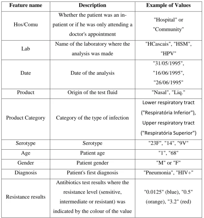
The dataset used in this project was collected from electronic health records for the purpose of reporting antibiotic resistance. It does not represent the full EHR for each patient, but the data thought necessary to report. It was collected from 33 different Portuguese hospitals between 1993 and 2005, yielding a total of 5118 entries. The data was made available in spreadsheet files. These are its main features, including a description and examples of values in Table 3.1.1:

 Whether the patient was an in-patient or if he was only attending a doctor's appointment

 Name of the laboratory where the analysis was made

 Date of the analysis

 Origin of the test fluid

 Category of the type of infection

 Serotype

 Patient age

 Patient gender

 Patient's first diagnosis

12

Feature name Description Example of Values

Hos/Comu

Whether the patient was an in-patient or if he was only attending a

doctor's appointment

"Hospital" or "Community"

Lab Name of the laboratory where the analysis was made

"HCascais", "HSM", "HPV"

Date Date of the analysis

"31/05/1995", "16/06/1995", "26/06/1995" Product Origin of the test fluid "Nasal", "Liq."

Product Category Category of the type of infection

Lower respiratory tract ("Respiratória Inferior"),

Upper respiratory tract ("Respiratória Superior") Serotype Serotype "23F", "14", "9V"

Age Patient age "1", "68"

Gender Patient gender "M" or "F" Diagnosis Patient's first diagnosis "Pneumonia", "HIV+"

Resistance results

Antibiotics test results where the resistance level (sensitive, intermediate or resistant) was indicated by the colour of the value

"0.0125" (blue), "0.5" (orange), "3.2" (red)

Table 3.1.1: Main features of the dataset

Each patient was tested for 10 different antibiotics: Penicillin, Tetramycin, Erythromycin, Clindamycin, Chloramphenicol, Ofloxacin, Cefotaxime, Ceftriaxone, SXT and OXA.

13

3.2 Data Cleaning and Normalization

Several entries did not have resistance values for any of the antibiotics, and were therefore removed. From the original 5118 entries, 3813 remained after this step. Although several of the remaining entries had missing values, such as the patient's age or gender, or the origin of the test fluid, they were kept because the loss of vital information was minimal.

Some data features were also normalized. It was noticed that the data contained heterogeneous labels due to lack of coherence since it was collected by different staff (i.e., different ways to write the patient's age or the hospital name). Consequently, there was a need to check every different notation that referred to the same thing and change these entries so that they matched.

Furthermore, since the frontier values for the antibiotic resistance categories (resistant, intermediate or sensitive) vary from each antibiotic and the only way to know in which category a patient fit in was by checking the color that was given to its antibiotic resistance value, there was a need to create a new feature for each antibiotic that indicated if a patient showed resistance.

3.3 Data Transformation

All hospitals were labelled according to their NUTS II region (see Figure 3.3.1). Test fluids were grouped into probable infection types, according to expert validation. The patient's age were transformed into different age categories, e.g. 5 year slots, children vs. adults.

These transformed entries were added to the dataset as new features due to their probable relevance for the classification.

Besides these transformations, the antibiotics were also grouped by similarity in antibiotic families. These were the aggregations made:

 OXA and Penicillin

 Erythromycin and Clindamycin

14

Figure 3.3.1: NUTS II Regions of Portugal

It was established that if a patient showed resistance to any of the antibiotics of the family then the patient would be resistant to the family. By having the antibiotics grouped by families, new possibilities of finding interesting patterns may arouse.

3.4 Classification by Antibiotic

In a first step, classification of each patient as resistant or susceptible to each antibiotic individually was performed. Each patient was taken as an instance, described with the following attributes:

 Whether the patient was an in-patient or if he was only attending a doctor's appointment

 Region of the laboratory where the analysis was made

 Date of the analysis

 Origin of the test fluid

 Category of the type of infection

15

 Patient age

 Patient gender

 Antibiotics test results

WEKA 3.7.12 [20] was employed, due to its widespread use and its simplicity. In a first approach, it was decided to apply the Decision Tables (DT), Random Forests (RF), Multilayer Perceptron (MP) and Support Vector Machines (SVM) [21] algorithms, in a 10-fold cross validation. These algorithms represent a selection based on simplicity and readability of results (DT, RF) and performance reported in other biomedical informatics tasks (SVM, MP).

A Decision Table is a tabular form for displaying decision logic [22]. Random Forest is an ensemble of unpruned classification or regression trees created by using bootstrap samples of the training data and random feature selection in tree induction where prediction is made by aggregating the predictions of the ensemble [23]. The Multilayer Perceptron consists of a system of simple interconnected neurons, or nodes, which is a model representing a nonlinear mapping between an input vector and an output vector [24]. A Support Vector Machine is an algorithm that learns by example to assign labels to objects [25]. The parameters used in each algorithm can be consulted in Appendix I.

Since class imbalance was detected, the SMOTE [26] and Spread Subsample [27] filters were also tested. The SMOTE filter consists on over-sampling the minority class by creating similar (not equal) instances. Using a SMOTE filter with a percentage of 200% means that the amount of new SMOTE instances to be created is twice the number of instances of the minority class. On the other hand, the Spread Subsample filter produces a random subsample of the dataset, where the ratio between the frequency of classes can be defined.

Afterwards, an Information Gain Attribute Evaluation was performed, in order to test classification using only the most relevant features. The algorithms and filters used for this test were the same as before.

Finally, similar tests were made for the antibiotic families mentioned in section 3.3, using all relevant features and Decision Tables without any filter applied and with the same filters previously used (SMOTE and Spread Subsample, both with the same settings as before).

16

3.5 Antibiotic Resistance Profiling

The next approach was to test classification by resistance profile. Clustering techniques were applied to identify resistance profiles, i.e. patients that showed resistance to the same set of antibiotics.

By making use of WEKA once again, an expectation-maximization algorithm was used over the patient instances whose features consisted only on antibiotic resistance values in order to assign a probability distribution to each instance which indicates the probability of it belonging to each of the clusters. The number of clusters was selected automatically by cross-validation. Each resulting cluster represented a different resistance profile.

3.6 Classification by Resistance Profile

The classes for each instance were then altered to one of the identified resistance profiles. An ID was also added for instance identification purposes, but it was disregarded in every classification test.

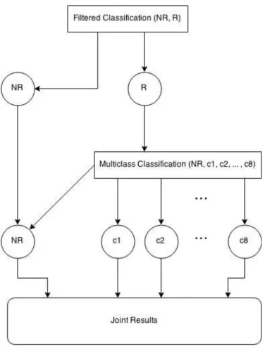
After that, a two-stage classification strategy was devised in order to classify patients according to their resistance profile. Figure 3.6.1 is an illustration of how it works.

For the first step, the filtered classification, a two class classification strategy was employed, where all the instances belonging to clusters of resistant profiles were grouped into a single class (R), whereas patients without any resistance were grouped into another class (NR). The filtered classification was always done with a SMOTE filter with a percentage of SMOTE instances to create of 500% and the classification algorithms tested were Decision Tables and Random Forests with a 10-fold cross-validation.

17

Figure 3.6.1: Two-stage classification strategy architecture

Next, the instances that were classified as Resistant, had their "original" profile classifications reassigned, meaning, the ones that were predicted by the expectation-maximization algorithm. Hence the importance of having an ID, so that the predicted instances can be traced back to the original input file so that their cluster can be retrieved. Instances classified as Non-resistant, were removed from the dataset.

Afterwards, those same instances were classified via Multiclass Classification, so that the multi-class dataset could be handled with 2-class classifiers. The classification algorithms used were again Decision Tables and Random Forests, always with 10-fold cross-validation, and the methods used for transforming the multi-class problem into several 2-class ones were 1-against-all and 1-against-1.

The difference between these two methods is that, while 1-against-all takes one class and tests it against all the remaining ones, 1-against-1 does the same, but only against one at a time, repeating the procedure until all the possibilities have been covered.

18

Finally, the precision, recall and F-measure were compiled so that the different algorithm tests could be compared. The following formulas illustrate how each of these metrics is calculated:

The tp refers to true positives, whereas the fp refers to false positives and fn to false negatives. Establishing a connection between these terms and our problem we would have:

 True positive - number of correct classifications from positive examples

 True negative - number of correct classifications from negative examples

 False positive - number of incorrect classifications from positive examples

 False negative - number of incorrect classifications from negative examples

Another approach tested was based on a direct classification of instances into resistance profiles, correcting some of the erroneous cluster assignments made by the clustering algorithm. Instances wrongly assigned to a cluster were reassigned. A new cluster named "cluster 9" was created for the cases in which an instance did not fit in any of the already existing clusters (for instance, if the patient only showed resistance to SXT). Then, the entire process described in Figure 3.2 was repeated using this new data set.

Finally, yet another approach was tested, one that, besides the information used in the previous ones, included a newly created compound feature: the number of instances belonging to each cluster in the current month. The same tests as before were performed using this dataset with the month values information.

19

3.7 Time Series

After all the classification tests were done, both by antibiotic and resistance profile, a new dataset was devised, where each instance represented a month and whose features relate to the number of patients that belonged to cluster on the corresponding month, so that time series analysis and forecasting could be performed over it. This would allow to make predictions of the evolution of the number of patients belonging to a certain antibiotic resistance profile.

The algorithms used for the base learner were Decision Tables and Random Forests, due to their previous usage in the project and time constraints. The tests were evaluated on training, the periodicity was left unknown, and the predictions were made one-step-ahead.

21

Chapter 4

Results

In this section, the results of the cleaning and normalization tasks, as well as the classification tests will be presented.

4.1 Data Normalization and Transformation

As it was previously mentioned in sections 3.2 and 3.3, after receiving the data set that would support the work, I proceeded to analyze it and perform data cleaning and normalization. After the deletion of the entries that had vital information missing, some data features were normalized to cope with their heterogeneous labels.

Table 4.1.1 shows a few examples of entries that were normalized, and the changes that resulted from it.

Feature

Original entries

Normalized entries

Hospital name "HVFXira" "HVFXira" "HFXira" "HCUF" "CUF" "CUF"

Origin of the test fluid

"LIQ. ?" "Liq." "Liq?" "Liq." "NAS" "Nasal" "Nasal"

22

Afterwards, some features were transformed in order to group them by expert categories. Some examples that illustrate the changes that derived from the data transformation can be seen in Table 4.1.2.

Feature Description Original entries Transformed entries

Location The hospitals were grouped by their NUTS II region

INSA Lisbon ("Lisboa") HSM INSP North ("Norte") HVNG

Date The entries' season was derived from their date

31/05/1995 Spring ("Primavera") 16/06/1995 26/06/1995 Summer ("Verão") 28/06/1995 Origin of the test fluid

Grouped into categories by probable infection type

Bronchial secretion ("Secreção Brônquica") Lower respiratory tract ("Respiratória Inferior") Bronchial lavage ("Lavado Brônquico")

Nasal ("Nasal") Upper respiratory tract ("Respiratória

Superior") Nasopharyngeal

("Nasofaringeal")

Patient age

Grouped into several age categories (children vs. adults

and year slots)

1

"C" and "1-2A" 2

18

"A" and "18-50A" 33

Antibiotic test results

The entries were split into Resistant or Non-Resistant according to the colours their

numeric values showed

Blue values Resistant ("Resistente") Yellow values

Red values Non-Resistant ("Não Resistente")

23

4.2 Statistical Analysis

To have a better perception of the dataset that supported this project, a thorough statistical analysis was made.

First of all, it was important to know how many blank entries were found in each of the relevant features of the dataset (see Table 4.2.1).

Number of blank entries in each relevant feature

Feature

Number of blank entries

Inpatient or ambulatory patient 1997 (52.57%)

Laboratory name 0 (0%)

Analysis date 28 (0.73%)

Origin of the test fluid 110 (2.88%)

Category of the type of infection 110 (2.88%)

Serotype 2025 (53.11%)

Patient age 582 (15.26%)

Patient gender 1282 (33.62%)

Patient's first diagnosis 3582 (93.94%)

Antibiotics test results 0 (0%)

Table 4.2.1: Number of blank entries in each relevant feature

A first analysis clearly showed that the patient's first diagnosis, having over 90% of its entries blank, is not a suitable feature to work with and was consequently discarded. Other features, such as whether the patient was an in-patient or if he was only attending a doctor's appointment or the serotype showed about half blank entries. Although a significant number, they could still be proven useful and were therefore kept for the classification.

Although the dataset has patients from 6 different regions, over 90% of these are from either Lisbon or the North. This means that it will be hard to draw any conclusions regarding any of the remaining 4 regions (Alentejo, Algarve, Madeira and Center).

24

The entries are evenly distributed throughout all the years from 1994 to 2004. There are less entries from 1993 and 2005, since these are the border years of the dataset. The same goes for months and seasons, which is very good, as it shows that the dataset is continuous and may allow to examine if there are interesting patterns by season, or if there were any antibiotic resistance peaks and try to infer why, for example.

Around two thirds of the patients were adults and around the same percentage were male. Figure 4.2.1 illustrates how many patients showed resistance to each antibiotic, out of all the 3813 entries:

Figure 4.2.1: Resistant patients by antibiotic

At a first glance, there data seems to have a class imbalance problem for all antibiotics, since the number of patients that show resistance to any of them is a lot smaller that the number of patients that do not.

4.3 Classification by Antibiotic

In the individual antibiotic classification task, Decision Tables, Random Forests, Support Vector Machines and Multilayer Perceptron were applied without any filters.

3.20% 14.98% 12.96% 9.36% 6.61% 0.37% 1.70% 0.60% 1.26% 1.63% 0 100 200 300 400 500 600

Resistant Patients by Antibiotic

25

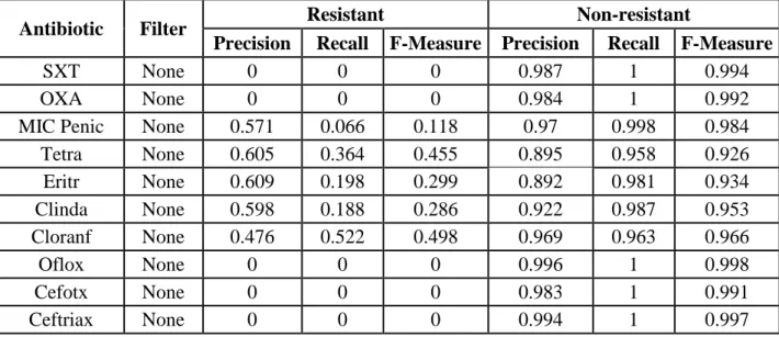
Table 4.3.1 shows the precision, recall and F-measure results for the tests using Decision Tables with a 10-fold cross-validation for every antibiotic.

Antibiotic Filter Resistant Non-resistant

Precision Recall F-Measure Precision Recall F-Measure

SXT None 0 0 0 0.987 1 0.994

OXA None 0 0 0 0.984 1 0.992

MIC Penic None 0.571 0.066 0.118 0.97 0.998 0.984

Tetra None 0.605 0.364 0.455 0.895 0.958 0.926 Eritr None 0.609 0.198 0.299 0.892 0.981 0.934 Clinda None 0.598 0.188 0.286 0.922 0.987 0.953 Cloranf None 0.476 0.522 0.498 0.969 0.963 0.966 Oflox None 0 0 0 0.996 1 0.998 Cefotx None 0 0 0 0.983 1 0.991 Ceftriax None 0 0 0 0.994 1 0.997

Table 4.3.1: Classification by antibiotic results using Decision Tables

The results using Random Forests, Support Vector Machines and Multilayer Perceptron with a 10-fold cross-validation for Tetramycin, seeing as it was one antibiotics with best results in the table above, can be seen on Table 4.3.2.

Antibiotic Algorithm Resistant Non-resistant

Precision Recall F-Measure Precision Recall F-Measure

Tetra Random

Forests 0.800 0.056 0.105 0.857 0.998 0.992

Tetra SVM 0 0 0 0.850 1 0.919

Tetra Multilayer

Perceptron 0.492 0.382 0.430 0.895 0.931 0.913

Table 4.3.2: Classification results for Tetramycin using other algorithms

From these results it was obvious the there was a class imbalance problem, due to the number of non-resistant patients being much higher than the number of resistant ones. This lead to most of the already few resistant patients being classified as

non-26

resistant. Hence the very high accuracy regarding the non-resistant patients, and the opposite regarding those that showed resistance.

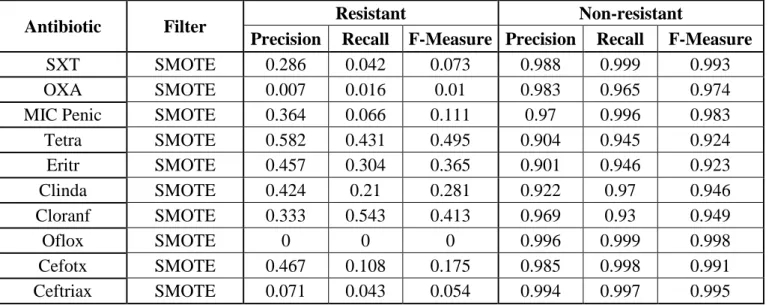
In order to counter this class imbalance problem, two different filters were used with filtered classifying: SMOTE at 200% (see Tables 4.3.3 and 4.3.4) and Spread Subsample with a uniform distribution (see Tables 4.3.5 and 4.3.6).

SMOTE (with a percentage of 200)

Antibiotic Filter Resistant Non-resistant

Precision Recall F-Measure Precision Recall F-Measure

SXT SMOTE 0.286 0.042 0.073 0.988 0.999 0.993

OXA SMOTE 0.007 0.016 0.01 0.983 0.965 0.974

MIC Penic SMOTE 0.364 0.066 0.111 0.97 0.996 0.983

Tetra SMOTE 0.582 0.431 0.495 0.904 0.945 0.924 Eritr SMOTE 0.457 0.304 0.365 0.901 0.946 0.923 Clinda SMOTE 0.424 0.21 0.281 0.922 0.97 0.946 Cloranf SMOTE 0.333 0.543 0.413 0.969 0.93 0.949 Oflox SMOTE 0 0 0 0.996 0.999 0.998 Cefotx SMOTE 0.467 0.108 0.175 0.985 0.998 0.991 Ceftriax SMOTE 0.071 0.043 0.054 0.994 0.997 0.995

Table 4.3.3: Classification by antibiotic results using Decision Tables with a SMOTE filter (200%)

Antibiotic Algorithm Resistant Non-resistant

Precision Recall F-Measure Precision Recall F-Measure

Tetra Random Forests 0.650 0.068 0.124 0.858 0.994 0.921

Tetra SVM 0.366 0.112 0.172 0.861 0.966 0.919

Tetra Multilayer

Perceptron 0.504 0.419 0.457 0.901 0.928 0.914

Table 4.3.4: Classification results for Tetramycin using other algorithms with a SMOTE filter (200%)

27

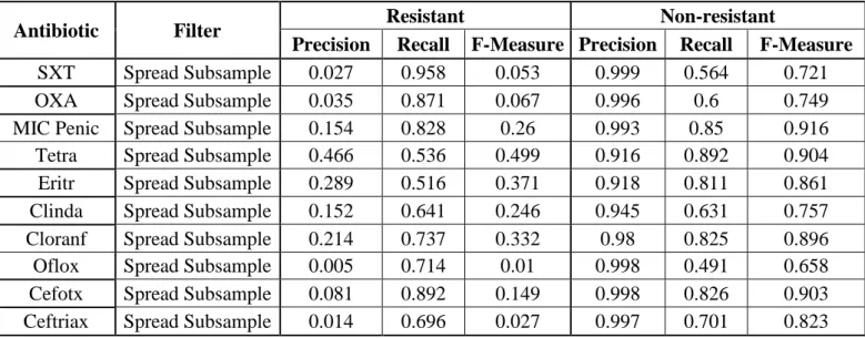
Spread Subsample (with a distribution spread of 1)

Antibiotic Filter Resistant Non-resistant

Precision Recall F-Measure Precision Recall F-Measure

SXT Spread Subsample 0.027 0.958 0.053 0.999 0.564 0.721

OXA Spread Subsample 0.035 0.871 0.067 0.996 0.6 0.749

MIC Penic Spread Subsample 0.154 0.828 0.26 0.993 0.85 0.916

Tetra Spread Subsample 0.466 0.536 0.499 0.916 0.892 0.904

Eritr Spread Subsample 0.289 0.516 0.371 0.918 0.811 0.861

Clinda Spread Subsample 0.152 0.641 0.246 0.945 0.631 0.757

Cloranf Spread Subsample 0.214 0.737 0.332 0.98 0.825 0.896

Oflox Spread Subsample 0.005 0.714 0.01 0.998 0.491 0.658

Cefotx Spread Subsample 0.081 0.892 0.149 0.998 0.826 0.903 Ceftriax Spread Subsample 0.014 0.696 0.027 0.997 0.701 0.823

Table 4.3.5: Classification by antibiotic results using Decision Tables with a Spread Subsample filter

Antibiotic Algorithm Resistant Non-resistant

Precision Recall F-Measure Precision Recall F-Measure

Tetra Random Forests 0.235 0.445 0.307 0.884 0.744 0.808

Tetra SVM 0.223 0.518 0.312 0.889 0.682 0.772

Tetra Multilayer

Perceptron 0.265 0.660 0.378 0.919 0.677 0.780

Table 4.3.6: Classification results for Tetramycin using other algorithms with a Spread Subsample filter

The results show that the SMOTE filter brought some improvements, but not enough to be considered a valid option. As for the Spread Subsample filter, the recall raised significantly, but at the expense of a great reduction on the precision in most cases.

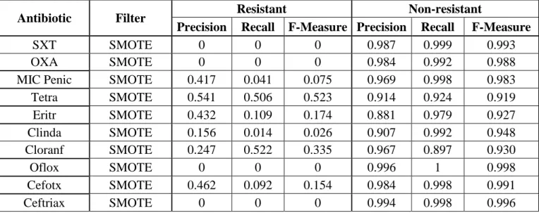
Since some improvements were verified when testing with a SMOTE filter with a percentage of SMOTE instances of 200, another test was made with a higher percentage (500%). On average this improved the F-measure but overall performance was still very low (see Tables 4.3.7 and 4.3.8).

28 SMOTE (with a percentage of 500)

Antibiotic Filter Resistant Non-resistant

Precision Recall F-Measure Precision Recall F-Measure

SXT SMOTE 0 0 0 0.987 0.999 0.993

OXA SMOTE 0 0 0 0.984 0.992 0.988

MIC Penic SMOTE 0.417 0.041 0.075 0.969 0.998 0.983

Tetra SMOTE 0.541 0.506 0.523 0.914 0.924 0.919 Eritr SMOTE 0.432 0.109 0.174 0.881 0.979 0.927 Clinda SMOTE 0.156 0.014 0.026 0.907 0.992 0.948 Cloranf SMOTE 0.247 0.522 0.335 0.967 0.897 0.930 Oflox SMOTE 0 0 0 0.996 1 0.998 Cefotx SMOTE 0.462 0.092 0.154 0.984 0.998 0.991 Ceftriax SMOTE 0 0 0 0.994 0.998 0.996

Table 4.3.7: Classification by antibiotic results using Decision Tables with a SMOTE filter (500%)

Antibiotic Algorithm Resistant Non-resistant

Precision Recall F-Measure Precision Recall F-Measure

Tetra Random Forests 0.505 0.082 0.142 0.859 0.986 0.918

Tetra SVM 0.262 0.356 0.302 0.879 0.824 0.851

Tetra Multilayer

Perceptron 0.484 0.420 0.450 0.900 0.921 0.911

Table 4.3.8: Classification results for Tetramycin using other algorithms with a SMOTE filter (500%)

Due to the low performance of the tests made until then, an Information Gain Attribute Evaluation was performed to find the most relevant features. These were the 6 most relevant ones:

 Region where the analysis was made

 Month

 Category of the type of infection

 Serotype

 Patient age

29

The same four algorithms and filters as before were tested over this new dataset with less features. The SMOTE filter was performed with a percentage of 500%, due to the slightly better results compared with the ones with a percentage of 200% on the previous tests. The results obtained for Tetramycin are shown in Table 4.3.9.

Algorithm Filter Resistant Non-resistant

Precision Recall F-Measure Precision Recall F-Measure

Decision Tables None 0.611 0.361 0.454 0.895 0.960 0.926 SMOTE 0.512 0.506 0.509 0.913 0.915 0.914 Spread Subsample 0.466 0.536 0.499 0.916 0.892 0.904 Random Forests None 0.694 0.075 0.136 0.859 0.994 0.922 SMOTE 0.305 0.159 0.209 0.863 0.936 0.898 Spread Subsample 0.228 0.455 0.304 0.884 0.728 0.798 SVM None 0 0 0 0.850 1 0.919 SMOTE 0.330 0.306 0.318 0.879 0.890 0.885 Spread Subsample 0.226 0.494 0.310 0.887 0.702 0.784 Multilayer Perceptron None 0.501 0.320 0.391 0.887 0.944 0.915 SMOTE 0.471 0.401 0.433 0.897 0.921 0.909 Spread Subsample 0.233 0.646 0.342 0.909 0.625 0.741

Table 4.3.9: Classification results for Tetramycin using feature selection

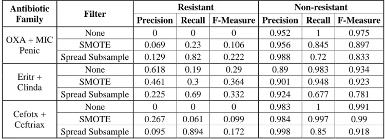
As it was mentioned in the previous section, some antibiotics were also grouped by similarity in antibiotic families. These families were also tested the same way the antibiotics were. Table 4.3.10 shows the results for each antibiotic tested with Decision Tables without any filter applied and with the same filters as before.

Antibiotic

Family Filter

Resistant Non-resistant

Precision Recall F-Measure Precision Recall F-Measure

OXA + MIC Penic None 0 0 0 0.952 1 0.975 SMOTE 0.069 0.23 0.106 0.956 0.845 0.897 Spread Subsample 0.129 0.82 0.222 0.988 0.72 0.833 Eritr + Clinda None 0.618 0.19 0.29 0.89 0.983 0.934 SMOTE 0.461 0.3 0.364 0.901 0.948 0.923 Spread Subsample 0.225 0.69 0.332 0.924 0.677 0.781 Cefotx + Ceftriax None 0 0 0 0.983 1 0.991 SMOTE 0.267 0.061 0.099 0.984 0.997 0.99 Spread Subsample 0.095 0.894 0.172 0.998 0.85 0.918

30

The results were very similar to the ones when the antibiotics were tested separately.

4.4 Antibiotic Resistance Profiling

In an attempt to overcome the low performance observed in classification by individual antibiotic resistance or family, a new strategy was devised based on a three step approach:

1. Instances were clustered into resistance profiles;

2. Instances were classified as resistant (resistant to at least one antibiotic) and non-resistant (to all);

3. Resistant classified instances were re-classified in a multiclass approach to the resistance profiles.

The instances were divided in 9 different clusters. Their profiles and how many instances were clustered into each one of them can be consulted in Table 4.4.1 and Figure 4.4.1, respectively.

Cluster Resistant to

Cluster 0 None

Cluster 1 Tetramycin, Erythromycin, Clindamycin and Chloramphenicol

Cluster 2 Erythromycin

Cluster 3 Erythromycin and Clindamycin

Cluster 4 Penicillin, Tetramycin, Clindamycin and Cefotaxime

Cluster 5 OXA

Cluster 6 Tetramycin, Erythromycin and Clindamycin

Cluster 7 Tetramycin and Chloramphenicol

Cluster 8 Penicillin and Cefotaxime

31

Figure 4.4.1: Clustered instances by cluster

4.5 Classification by Profile Resistance

After these clusters were made, the two-stage classification strategy previously described in section 3.6 was tested. Given the algorithm performances for the classification by antibiotic (section 4.3), Support Vector Machines and Multilayer Perceptron were discarded. The first due to its unsatisfying results, and the second because of computational power and time constraints. For the filtered classification step, a SMOTE filter with a percentage of 500% was used.

Table 4.5.1 shows the results for the filtered classification step of the two-stage classification strategy.

Algorithm Cluster 0 Cluster 1

Precision Recall F-Measure Precision Recall F-Measure

Decision Table 0.897 0.888 0.892 0.503 0.526 0.514

Random Forest 0.835 0.977 0.901 0.5 0.106 0.175

Table 4.5.1: Classification results for the first step of the two-stage classification strategy without cluster adjustment

82.24% 1.76% 3.20% 1.47% 0.45% 0.37% 6.01% 3.46% 1.05% 0 500 1000 1500 2000 2500 3000 3500 Cluster

0 Cluster 1 Cluster 2 Cluster 3 Cluster 4 Cluster 5 Cluster 6 Cluster 7 Cluster 8

Clustered Instances by Cluster

32

Then, after the instances predicted into Cluster 1 were give their original clusters back, they were classified with multiclass classification (1-against-all and 1-against-1), using the same algorithms that were used in the filtered classification. The results for the multiclass classification with Random Forests after the filtered classification with Decision Tables, seeing as it was the algorithm with the best results, can be consulted in Table 4.5.2.

Cluster 1-against-all 1-against-1

Precision Recall F-Measure Precision Recall F-Measure

Cluster 0 0.595 0.786 0.677 0.588 0.839 0.691 Cluster 1 0.1 0.024 0.038 0 0 0 Cluster 2 0.25 0.136 0.176 0.381 0.136 0.2 Cluster 3 0.333 0.148 0.205 0.429 0.111 0.176 Cluster 4 0.5 0.25 0.333 0.571 0.25 0.348 Cluster 5 0 0 0 0 0 0 Cluster 6 0.408 0.333 0.367 0.507 0.376 0.432 Cluster 7 0.605 0.69 0.645 0.609 0.67 0.638 Cluster 8 0 0 0 0 0 0

Table 4.5.2: Classification results for the second step of the two-stage classification strategy without cluster adjustment

The outcomes of the tests with each of the other algorithms were similar.

Next, classification by resistance profile was tested again, only this time discarding the prediction errors when grouping the instances into clusters, as it was explained in the previous section. Figure 4.5.1 shows the number of clustered instances in each cluster after this cluster adjustment. The results for the filtered classification step using the new dataset are shown in Table 4.5.3.

33

Figure 4.5.1: Clustered instances by cluster after cluster adjustment

Algorithm Cluster 0 Cluster 1

Precision Recall F-Measure Precision Recall F-Measure

Decision Table 0.864 0.854 0.859 0.538 0.56 0.549

Random Forest 0.784 0.958 0.862 0.485 0.131 0.207

Table 4.5.3: Classification results for the first step of the two-stage classification strategy with cluster adjustment

The results for the patients resistant to any antibiotic (Cluster 1) improved slightly when compared to the previous approach, where the clustering prediction errors were not corrected.

As for the multiclass classification, the Random Forest showed better results than those from the Decision Tables (see Table 4.5.4).

76.66% 1.34% 2.02% 1.31% 0.24% 0.87% 5.46% 2.44% 0.55% 9.13% 0 500 1000 1500 2000 2500 3000 3500

Number of Clustered Instances