CONDITIONAL MODELS IN PERFORMANCE EVALUATION OF INVESTMENT FUNDS IN PORTUGAL: SELECTIVITY AND MARKET
TIMING (DAILY vs. MONTHLY ANALYSIS)
Osvaldo Afonso
PhD student in Economic & Mangement Sciences Faculty of Economics, University of Algarve
Paulo M. M. Rodrigues Universidade Nova de Lisboa
Banco de Portugal
CEFAGE (UE) – Center for Advanced Studies in Management and Economics, University of Évora
Cristina Viegas
Faculty of Economics, University of Algarve
CEFAGE (UE) – Center for Advanced Studies in Management and Economics, University of Évora
PRELIMINARY VERSION
CONDITIONAL MODELS IN PERFORMANCE EVALUATION OF INVESTMENT FUNDS IN PORTUGAL: SELECTIVITY AND MARKET
TIMING (DAILY vs. MONTHLY ANALYSIS)
ABSTRACT
Investment funds’ performance evaluation is one area of finance which has observed many developments over the past 40 years. In this field, traditional techniques of evaluation have not made use of models of conditional returns. These approaches do not allow for the temporal dependence of expected returns. To overcome this problem, Ferson and Schadt (1996) developed a new conditional performance evaluation approach.
The present work applies the methodology of Ferson and Schadt (1996) on a sample of 32 Portuguese investment funds observed from 31 December 2005 to 31 December 2013, with the objective to evaluate the performance of these investment funds, in the terms of selectivity and market timing, based on daily and monthly data.
Key Words: Conditional Performance Evaluation, Selectivity, Market Timing,
1. Introduction
The high growth and development which reached the investment fund industry in major financial markets and, in particular, in Portugal, justifies the importance of assessing the performance of a portfolio of securities.
Performance evaluation of investment funds has a long history. In the 1980s, a great interest emerged on the separation of the results of the performance of investment funds into two components: selectivity (stock picking) and market-timing.
This interest was reinforced by the work of Henriksson and Merton (1981) which complements the results of Treynor and Mazuy (1966). These authors, using Jensen´s alpha, present a method that allows decomposing the overall profitability obtained into two components: one relating to selectivity and the other to market-timing. The first component concerns the possibility of the manager selecting individually the various financial assets. The second component refers to the ability of the manager, given the cyclical movements of the market, to readjust the composition of the portfolio.
In the literature, many studies have applied the models of Treynor and Mazuy (1966) and Henriksson and Merton (1981) to test the abilities of selectivity and market timing in investment funds/managers. The empirical evidence so far is mixed: many of these studies conclude that investment funds/managers have no market timing capacity [see, e.g., Athanassakos, Caraynnopoulos and Racine (2002), Romacho (2003), Chen et al. (2013), Christensen (2013), Lonkani, Satjawathee e Jegasothy (2013) and Skrinjaric (2013)]; and others find evidence that some funds/managers have the capacity of selectivity [see, e.g., Fletcher (1995) and Heaney and Josev (2005), and Chen et al. (2013)]. It has also been shown in the literature that funds have perverse market timing skills [see, e.g., Kon (1983), Chang Lewellen (1984) and Jagannathan and Korajczyk (1986)]. However, in the literature, there have also been studies where managers have shown a positive market timing capacity [see, e.g., Bollen and Busse (2001), Chance and Hemler (2001), Laplante (2003), Jiang, Yao and Yu (2007), Amman and Zingg (2008) and Raju and Rao (2009)].
In the mid-nineties of the last century, conditional models that assume the existence of information on the state of the economy with impact on expected returns are proposed. These models allow for the evaluation of the performance to be measured more effectively when expected returns are affected by deterministics, than when this does not happen [see, e.g., Ferson and Korajczyk (1995), Chen and Knez (1996), Ferson and Warther (1996) and Christopherson, Ferson and Glassman (1998)]. In this context, Ferson and Schadt (1996) developed a theoretical framework for the conditional models of Sharpe (1964), Treynor and Mazuy (1966) and Henriksson and Merton (1981).
In the financial literature several studies on different markets have emerged, where these conditional models have been applied, [see, e.g., Roy and Deb (2004), Aragon (2005), Heaney and Josev (2005), Leite and Cortez (2009), Afonso (2010), Bodson, Cavenaile and Sougné (2013) and Chen et al. (2013)]. These studies demonstrate that conditional models improve the capacities of detecting selectivity and market timing of funds/managers in relation to unconditional models1.
The overall objective of this work is to determine and to exploit the potential of conditional information models in the evaluation of the performance of investment funds. More specifically, the first objective is to verify, through conditional models, the capacities (daily and monthly) of selectivity and market timing of investment funds managers/securities belonging to the Portuguese market. The second objective is to ascertain which periodicity (daily or monthly) is the most efficient for analysing selectivity and market timing.
This article is organized as follows. Section 2, addresses the methodological procedures. Section 3, describes the sample that will serve as the basis for the empirical study on the investment funds performance evaluation in Portugal; and presents the empirical results of selectivity and market timing obtained from the application of conditional models. Finally, section 4 presents the conclusions of the work.
1 In this context, Wang (2004), questions the validity of predetermined variables usually used in the
financial literature on performance conditioning. The author notes that the appropriate selection of variables of information is crucial for performance evaluation.
2. Methodology
In this section, the performance evaluation approaches proposed by Ferson and Schadt (1996), and by Henriksson and Merton (1981) and Treynor and Mazuy (1966) are introduced.
2.1 – A Model Based on the CAPM
Ferson and Schadt (1996) consider a conditional version of the Capital Asset Pricing Model (CAPM) of Sharpe (1964) such as,
( )
, 1 , 1 , 1 ,t+ = cm t mt+ + ct+ c Z R u R β , 1 ,..., 0 , ,..., 0 − = = T t N c (1a)(
uc,t+1Zt)
=0 E (1b)(
uc,t+1Rmt+1Zt)
=0 E (1c) where, Rc,t+1 is the excess return (with respect to a risk-free rate) of asset c in period t+1, Zt is a vector of instruments for the information available at time t, Rm,t+1 is the market excess return in period t+1, βc,m( )
Zt is the conditional beta of the market excess return of asset c at time t, and uc,t+1 is an error term.The efficient market assumption is ensured in equation (1b) and in equation (1c) it is considered that the coefficients of the conditional regression are defined byβc,m
( )
Zt . To consider the hypothesis that portfolio managers do not use more information thanZt, the beta of the portfolio,βc,m( )
Zt , is a function ofZt, such that:( )
t c c tm
c, Z b0 β´ z
β = + ′ (2)
In this equation, zt =Zt −E
( )
Z is a vector of deviations of Ztin relation to its unconditional expected value, andβ
c′ is a vector of dimension equal toZt. The coefficient b0c in (2) should be interpreted as the "average beta", that is, theunconditional mean of the conditional beta:E
(
βc,m( )
Zt)
2. The elements of
β
care the response of the conditional beta with respect to the determinants considered. Equations (1a), (1b), (1c) and (2) imply the following generating process for the managed portfolio’s return:[
, 1]
, 1 1 , 1 ,t+ = oc mt+ + c′ t mt+ + ct+ c b R z R u R β (3) where E(
uc,t+1rm,t+1Zt)
=0.Now consider a regression of the excess return of the portfolio on the market factor, with the lagged information:
(
, 1)
, 1 2 1 , 1 1 ,t+ = c + c mt+ + ′c t mt+ + ct+ c R z R R α δ δ ε (4) where,α
crepresents a measure of selectivity.Taking the relevant expectations in (4) and comparing with the result of (3), the model implies that:
α
c =0,δ
1c =b0c andδ
2c =β
c3.2.2 –The Henriksson and Merton’s Model (HMC)
Henriksson and Merton (1981) and Henriksson (1984) describe an alternative model of market-timing. In their model, the manager attempts to predict when the return of the market portfolio will exceed the risk-free rate. When the forecast is for an up market, the manager will adjust the portfolio to higher target betas. When the market forecast is pessimistic, a low target is used. Given this model, Henriksson and Merton show that if the manager can time the market, then the coefficient
γ
u, which represents the (unconditional) measure of the ability of market timing, in the following regression, is positive:[
, 1]
, 1 1 , 1 , + + + + + = c + c mt + u mt + ct t c b R R u R α γ (5)2 This interpretation is an approximation, since it ignores the higher-order terms in the Taylor expansion. 3 OLS estimation of the regression model imposes the same moment conditions as does Hanssen's (1982)
where
[
Rm,t+1]
+is defined as Max(
0,Rm,t+1)
. Henriksson and Merton interpret Max(
0,Rm,t+1)
as the payoff of an option on a market portfolio with an exercise price equal to that of a risk free asset4 .To extend the model of Henriksson and Merton (1981) to a conditional analysis, it is assumed that the manager attempts to predictum,t+1 =Rm,t+1−Ε
(
Rm,t+1Zt)
, the deviation from the expected excess return, conditional on public information. If the prediction is positive, the manager chooses the portfolio’s conditional beta asβ
up( )
zt =bup+B Zup′ t. If the prediction is negative, the manager choosesβ
d( )
Zt =bd +Bd( )
Zt .Using this model for the beta parameters of the portfolio and equation (1) for individual assets, it follows that,
[
, 1]
, 1[
, 1]
, 1 1 , 1 , + + ∗ + ∗ + + + = d mt + ′d t mt + c mt + ′ t mt + ct t c b R B z R R z R u R γ ∆ (6) where{
, 1(
, 1)
0}
1 , 1 ,+ = + + − + > ∗ t t m t m t m t m R R R Z R Ι Ε , γc =bup −bd,e ∆=Bup −Bd.{ }
•Ι is an indicator function. The coefficient
γ
c is the (conditional) measure of market timing skill. The null hypothesis of no market-timing ability implies thatγ
c and∆are zero. The alternative hypothesis of positive market-timing skill implies that0
> ′ + t
c
∆
zγ
. As soon as the conditional beta is higher when the market is above the conditional expectation, given the determinants considered, than when it is below the conditional expectation. This situation implies thatΕ(
γc+∆′zt)
=γc>0, which means thatmarket-timing is, on average, positive5
4 Henriksson and Merton proposed to regression (5) to separate the market-timing ability from security
selection ability. However, as the model of Treynor and Mazuy (1966) this separation is problematic as was illustrated by Jagannathan and Korajczyk (1986). In its turn, Glosten and Jagannathan (1994) provide conditions under which the sum of the market timing and selectivity, components of performance, may estimate correctly the average (unconditional) value added by the manager. This argument can be extended to a conditional model. The problem of survival in the sample of funds makes the measure of value added appears larger.
5 The derivation assumes that if
N c
xc, =1,..., are the weights of the portfolio manager,
then
(
)
0 1 ,t+ t = c cu Z xE where ui,t+1is the error term in equation (1). This means that the manager may
2.3 - The Model of Treynor and Mazuy (TMC)
The quadratic regression of Treynor and Mazuy (1966) corresponds to the classical market-timing regression:
2
, 1 , 1 , 1 , 1.
c t c c m t u m t c t
R + =α β+ R + +γ R + +u + (7)
Ferson and Schadt (1996) introduced the conditional version of Treynor and Mazuy’s (1966) regression:
(
)
[ ]
, 1 2 1 , 1 , , 1 , 1 ,t+ = c+ c mt+ + c t mt+ + c mt+ + ct+ c R C z R R u R α β γ (8)where the coefficient vector C´ccaptures the response of the managers beta parameter to the determinants zt. The term Cc,
(
z Rt m t, 1+)
, in equation (8), controls the effect of public information, which would bias the coefficient estimates in the original model of Treynor and Mazuy (1966). This new term, captures part of the quadratic term in the model of Treynor and Mazuy assigned to the determinants of returns. In the conditional model, the correlation of the beta parameters of the investment funds with the returns of the market, which can be assigned to the determinants, is not considered to reflect the ability of market timing.
the forecasts of managers are correct under the alternative hypothesis of market-timing ability. Second Henriksson and Merton (1981), if managers forecasts and the beta adjustments can be correct or incorrect with some fixed probabilities, then we can show that:plim(γc +∆)′Zt = E
{
βup( )Zt rm > E(rm Zt),Zt}−E{
βd( )Zt rm < E(rm Zt),Zt}
.3. Empirical Analysis
In this section, in addition to a description of the database, the objective is to present the main results obtained with the two conditional models, previously introduced.
3.1 – The Data
3.1.1 - The Sample
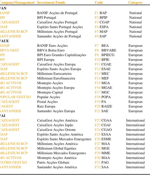
The sample used in this study is composed of 32 Portuguese Securities Investment Funds, classified according to the criteria of the Portuguese Association of Investment Funds, Pensions and Assets (APFIPP) as equity funds. These funds are divided into three categories: National, European Union and International.
The study period is from 31 December 2005 to 31 December 2013. Regarding the frequency of the data, daily and monthly returns were used6. The funds chosen are presented in Table 1. The performance evaluation of the funds was performed at the category and individual levels.
3.1.2 - Investment Funds Returns
For the calculation of the daily (monthly) returns of funds the value of the units of participation, obtained through the service for the dissemination of financial information Dathis, Euronext Lisbon7 is used. The daily (monthly) return of funds is calculated as,
= −1 ln c,t c,t c,t UP UP R (9) where c,t
R is the daily (monthly) return of fund c in period t; UPc,tis the value of the unit of participation of fund c in period t; UPc,t−1is the value of the unit of participation of fund c in period t-1.
6 All estimates and econometric calculations carried out in the study were obtained with the aid of the
Eviews program.
7
Table 1 – Investment Funds
CompanyManagement Investment Funds Code Category
FAN
BANIF BANIF Acções de Portugal F1 BAP National
BPI BPI Portugal F2 BPIP National
CAIXAGEST CaixaGest Acções Portugal F3 CGAP National
ESAF Espírito Santo Portugal Acções F4 ESPA National
MILLENIUM BCP Millenium Acções Portugal F5 MAP National
SANTANDER Santander Acções de Portugal F6 SAP National
FAUE
BANIF BANIF Euro Acções F7 BEA European
BBVA GEST BBVA Bolsa Euro F8 BBVABE European
BPI BPI Euro Grandes Capitalizações F9 BPIECG European
BPI BPI Europa F10 BPIE European
CAIXAGEST CaixaGest Acções Europa F11 CGAE European
ESAF Espírito Santo Acções Europa F12 ESAE European
MILLENIUM BCP Millenium Eurocarteira F13 MEC European
MILLENIUM BCP Millenium Eurofinanceira F14 MEF European
MG ACTIVOS Montepio Acções F15 MGA European
MG ACTIVOS Montepio Acções Europa F16 MGAE European
MG ACTIVOS Montepio Capital F17 MGC European
POPULAR GESTÃO Popular Acções F18 POPA European
CAIXAGEST Postal Acções F19 PA European
CAGEST Raiz Europa F20 RAIZE European
SANTANDER Santander Acções Europa F21 SAE European
FAI
CAIXAGEST CaixaGest Acções América F22 CGAA International
CAIXAGEST CaixaGest Acções Japão F23 CGAJ International
CAIXAGEST CaixaGest Acções Oriente F24 CGAO International
ESAF Espírito Santo Acções América F25 ESAA International
ESAF Espírito Santo Mercados Emergentes F26 ESME International
MILLENIUM BCP Millenium Acções América F27 MAA International
MILLENIUM BCP Millenium Global Equities F28 MGE International
MILLENIUM BCP Millenium Mercados Emergentes F29 MME International
MG ACTIVOS Montepio Acções América F30 MAA International
PATRIS GESTÃO Patris Acções Globais F31 PAG International
SANTANDER Santander Acções América F32 SAA International
3.1.3 - Market Return
For the calculation of the market return three indices, considered representative of the market portfolio of the three groups of funds that constitute the sample are used. For the funds of national assets the index PSI-20, obtained from the Euronext Lisbon is used. For European Union and International funds the indices MSCI Europe and MSCI World, obtained from Morgan Stanley Capital International were used.
Similarly as before, the market return is calculated as, = −1 , , , ln t m t m t m I I R (10) where t m
R , is the daily (Monthly) market return in period t; Im,tis the index value of the market in period t; and Im,t−1is the index value of the market in period t-1.
3.1.4 - The Risk Free Rate
Estimates of the risk-free asset rate are obtained from the series of returns of the Euribor (Euro Interbank Offered Rate) rate at 1 month obtained from the Bank of Portugal, which is converted to the daily and monthly rates as follows:
Daily Rate: + = 365 1 ln , a i t f R (11) Monthly Rate: + = 12 1 ln , a i t f R (12) where t f
R , is the risk free rate at time t; and ia is the Euribor rate for 1 month.
3.1.5 - Deterministics
Four different deterministics were used: (i) an indicator of inflation, (ii) a dummy variable for the month of January, (iii) a measure of the slope of the term structure of interest rates and (iv) an indicator of short-term interest rates. The study used a time lag of 1 day (month) for each variable of information.
Table 2 – Deterministics
Variables (Zt) Abbreviation Proxies Used
Inflation INF Observed Inflation: Consumer Price Index in Portugal
(annual rate of change).
January JAN Dummy with the value 1 when the month is a January and
of zero in remaining months.
Slope of Term STR Differential between the Rate of Return on Bonds and the
Interest Rate of Euribor at 3 months.
Interest Rate IR Variation of the Interest Rate of Euribor at 1 month.
Table 2 presents a description of the deterministics used (Zt).
Several empirical studies on the evaluation of the conditional performance of funds in international market (see, e.g.; Ferson and Schadt (1996), Christopherson, Ferson and Glassman (1998), Sawicki and Ong (2000), Ferson and Qian (2004)) and in the Portuguese market (see, e.g.; Cortez and Silva (2002), Leite and Cortez (2009) and Afonso (2010)) also applied some of these variables.
3.1.6 - Descriptive Statistics
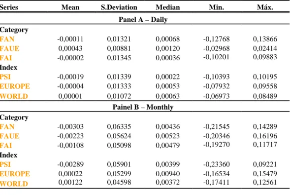
Table 3 presents a summary of the main descriptive statistics of returns (daily and monthly) for categories of funds and market indices.
Table 3 – Descriptive Statistics
Series Mean S.Deviation Median Min. Máx.
Panel A – Daily Category FAN -0,00011 0,01321 0,00068 -0,12768 0,13866 FAUE 0,00043 0,00881 0,00120 -0,02968 0,02414 FAI -0,00002 0,01345 0,00036 -0,10201 0,09883 Index PSI -0,00019 0,01339 0,00022 -0,10393 0,10195 EUROPE -0,00004 0,01333 0,00053 -0,07932 0,09558 WORLD 0,00001 0,01072 0,00063 -0,06973 0,08489 Painel B – Monthly Category FAN -0,00303 0,06335 0,00436 -0,21545 0,14289 FAUE -0,00223 0,05624 0,00523 -0,20346 0,16196 FAI -0,00108 0,05098 0,00479 -0,19270 0,11717 Index PSI -0,00289 0,05901 0,00399 -0,23360 0,09221 EUROPE 0,00022 0,05299 0,00940 -0,16534 0,15479 WORLD 0,00122 0,04598 0,00372 -0,17411 0,12561
A first observation from Table 3, is that it appears that the majority of categories of funds presents an average return (daily) exceeding the average return (daily) of the market index (with the exception of category FAI). On the other hand, it is also apparent that the volatility (daily and monthly) as measured by the standard deviation of categories is greater than the volatility (daily and monthly) of the market indices. Except for the volatility (daily) of categories FAN and FAUE which are lower than the volatility (daily) of the market index.
3.2 – Empirical Study: Selectivity (Stock Picking) and Market Timing
In this part the two components of the overall performance of investment funds is evaluated through the application of the conditional models of Henriksson and Merton (1981) and Treynor and Mazuy (1966). In order to correct for heteroscedasticity and autocorrelation detected by diagnostic tests the method of Newey-West (1987) is used.
3.2.1 - Conditional Model of Henriksson and Merton (HMC)
This point proceeds to the analysis of the results of the application of equation 6 (conditional model of Henriksson and Merton) which allows the evaluation of the skill of daily and monthly selectivity (α) and market timing (γ) of funds/managers.
3.2.1.1 - Selectivity and Market Timing of Categories of Funds
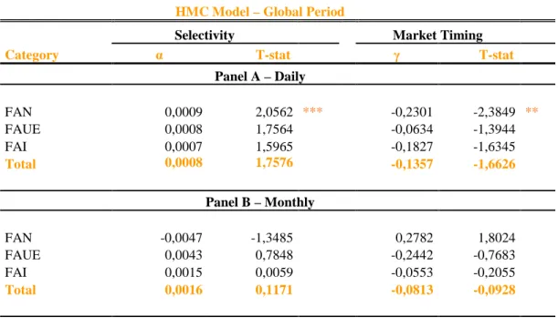
Table 4 shows, for each category of funds and for different frequencies of data (daily or monthly), the average estimates of the parameters α (selectivity) and γ (market timing) obtained with the conditioned model of Henriksson and Merton (HMC)).
Table 4 – Results for Selectivity and Market Timing of Categories (HMC Model)
HMC Model – Global Period
Selectivity Market Timing
Category α T-stat γ T-stat
Panel A – Daily FAN 0,0009 2,0562 *** -0,2301 -2,3849 ** FAUE 0,0008 1,7564 -0,0634 -1,3944 FAI 0,0007 1,5965 -0,1827 -1,6345 Total 0,0008 1,7576 -0,1357 -1,6626 Panel B – Monthly FAN -0,0047 -1,3485 0,2782 1,8024 FAUE 0,0043 0,7848 -0,2442 -0,7683 FAI 0,0015 0,0059 -0,0553 -0,2055 Total 0,0016 0,1171 -0,0813 -0,0928
Obs.: (i) α identifies the average selectivity and the γ identifies the average market timing; (ii) the symbols *, ** and *** indicate the level of significance of, respectively, 1%, 5% e 10%, according to the method of Newey-West (1987).
The results obtained show that, regardless of the category of funds and the frequency of returns (daily or monthly), these exhibit, on average, positive selectivity and market timing.
Panel A of Table 4 shows the results of the funds for daily data. A careful analysis of the results of panel A suggests that, in general, all categories of funds have positive coefficients of selectivity. The category of national funds is the one that presents worse ability in the selection of titles (0.09% per day), being statistically significant at a 10% significance level. With respect to market timing, measured by the parameter γ, the results indicate negative values for this coefficient in all categories of funds (the category of national funds obtains significant negative values at a 5% significance level). This is reflected in the average value of this coefficient (-0,1357). Conversely, the category of national funds obtains the worst performance in the coefficient of timing, with a mean value of -0,2031.
Panel B of Table 4 shows the results for monthly data. The categories of European and international funds have positive α parameter estimates, and for the category of national funds these are negative. Overall, it can be concluded that the results obtained (for daily or monthly data), through the conditional model of Henriksson and Merton (1981), supporting the hypothesis that the categories of funds have (tenuous) selectivity capacity, but not market timing (the exception being the category of monthly national funds).
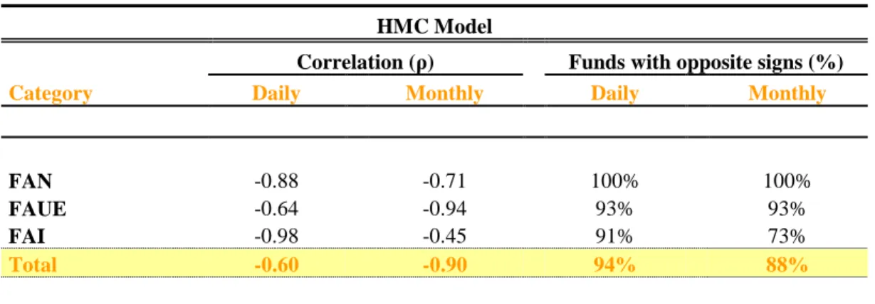
To support the observation that the funds with good performance in selectivity tend to have weak performance in market timing, correlation coefficients between funds categories were computed.
Table 5 – Correlation between Funds Categories (HMC Model)
HMC Model
Correlation (ρ) Funds with opposite signs (%)
Category Daily Monthly Daily Monthly
FAN -0.88 -0.71 100% 100% FAUE -0.64 -0.94 93% 93% FAI -0.98 -0.45 91% 73% Total -0.60 -0.90 94% 88%
Table 5 indicates a pronounced negative correlation (-0.60 and -0.90 for daily and monthly data, respectively) between selectivity and market timing. This table makes clear that, for the national and international funds, the use of daily data in the conditional HMC model can cause an increase of negative correlation. Finally, it should be noted, that the correlation coefficient goes from -0.88 to -0.71.
3.2.1.2 - Selectivity and Market Timing of Individual Funds (by Categories)
Table 6 reports the number of funds in each category, with positive and negative α and γ parameters, as well as the number of statistical significant funds.
With regard to the daily data (panel A), 30 funds (93.8 %) exhibit positive values of selectivity. For 19 of these funds (59.4 %) the selectivity coefficient, (α), is significantly greater than zero. Conversely, none of the two funds (6.3%) with negative values is statistically significant. With regards to the market timing ability, for 3 funds (9.4%), the coefficient associated with the capacity of market timing (γ) has a positive value (however, none is statistically significant). However, 29 funds (90.6%) present negative values for γ, of which 19 (59.4%) are significantly negative. Moreover, it is found that overall the F13 fund (category FAUE) obtains the best selectivity ability and the F21 fund (category FAUE) the best ability to predict the movements of the market8.
In relation to the results obtained with monthly data (panel B), 20 funds (62.5%) present positive estimates of selectivity, of which 8 are significantly positive. However, for 12 funds (37.5%) estimates of selectivity are negative, one of them being significantly negative. The ability of market timing was detected in 12 of the 32 funds (37.5 %) and of these, only 3 (9.4%) showed positive and significant coefficients. For the remaining 20 funds (62.5%) the values of the γ parameter are negative, and 1 (3.1%) of them significant. The F21 fund (category FAUE) obtains the best ability of selectivity and the F24 fund (category FAI) the best market timing ability.
8
Table 6 – Results of Selectivity and Market Timing of Individual Funds (HMC Model)
HMC Model – Global Period
Selectivity Market Timing
Category Nº Funds α > 0 α <0 γ > 0 γ <0 Panel A – Daily FAN 6 6 (4) 0 (0) 0 (0) 6 (6) FAUE 15 14 (9) 1 (0) 1 (0) 14 (7) 11 10 (6) 1 (0) 2 (0) 9 (6) FAI Total 32 30 (19) 2 (0) 3 (0) 29 (19) Panel B – Monthly FAN 6 0 (0) 6 (3) 6 (3) 0(0) FAUE 15 13 (1) 2 (0) 1 (0) 14(1) FAI 11 7 (0) 4 (0) 5 (0) 6(0) Total 32 20 (0) 13(3) 12 (3) 20(1)
Obs.: (i) α represents selectivity and γ market timing; (ii) the values between parentheses correspond to the number of funds with statistical significance.
In summary, the results obtained with the conditional HMC model, show that the funds included in the sample obtained better results in selectivity when daily data is used and market timing with monthly data.
3.2.2 - Conditional Model of Treynor and Mazuy (TMC)
At this point the results of applying equation 8 (conditional model of Treynor and Mazuy) are analyzed.
3.2.2.1 - Selectivity and Market Timing of Categories of Funds
Table 7 presents, for each category of funds and for different data frequencies (daily and/or monthly), the average estimates of α (selectivity) and γ (market timing) obtained from the conditional model of Treynor and Mazuy.
Table 7 – Results of Selectivity and Market Timing of Categories (TMC Model)
TMC Model –Global Period (2006/01 a 2013/12)
Selectivity Market Timing
Category Α T-stat γ T-stat
Panel A – Daily FAN 0,0004 1,3169 -3,1683 -3,6297 ** FAUE 0,0003 0,9140 -2,3888 -1,8386 FAI 0,0003 1,0775 -3,0117 -1,9588 Total 0,0011 0,8239 -2,7491 -2,2240 Panel B – Monthly FAN -0,0025 -1,0391 1,3104 2,5853 ** FAUE -0,0002 -0,1126 -0,5894 -0,4533 FAI 0,0002 0,0770 0,5804 0,4984 Total -0,0005 -0,2211 0,1689 0,4436
Obs.: (i) α represents the average selectivity and γ the average market timing; (ii) the symbols *, ** and
*** indicate the level of significance of, respectively, 1%, 5% e 10%, according to the method of Newey-West (1987).
The results obtained are similar to those obtained with the HMC model. The results show that, regardless of the category of funds and frequency (daily or monthly), the categories of funds exhibit on average negative selectivity and positive market timing. The exceptions are the international funds (category FAI) which present positive selectivity and market timing capacity.
Panel A of Table 7 presents the results of the funds for daily data. In general, all categories of funds have positive average estimates of α. The category of national funds (FAN) is the one that demonstrates better capacity for selection of titles (0.04% per day). However, it gets the worse performance in market timing, measured by γ, where the results indicate an average value of -3,1683. It should be noted that no category of funds gets positive estimates on selectivity and market timing simultaneously.
Panel B of Table 7 shows the results of the funds for monthly data. The categories of national (FAN) and European (FAUE) funds present estimates of α. Conversely, the category of international funds (FAI) obtains positive values for this coefficient. On the other hand, the categories of national (FAN) and international (FAI) funds exhibit
positive values for the market timing parameter (the category of national funds is statistically significant at a 5 % significance level).
In short, in global terms, it turns out that the daily results obtained support the hypothesis that the categories of funds have selectivity ability, but not market timing9. In turn, for the monthly results, the FAI category presents both selectivity and market timing ability.
In Table 8, in order to confirm that the funds with good performance in selectivity generally have a poor market timing performance, we calculated correlation coefficients between the categories of funds.
From the analysis of Table 8 we see that there is a pronounced negative correlation (-0.78 and -0.51 for daily and monthly data, respectively) between selectivity and market timing, indicating that managers who demonstrate ability for selectivity do not for market timing activities and vice versa. The most significant aspect that results from this table is that, for the category of national funds, it is indifferent to use daily or monthly data in the TMC model. This category of funds keeps the percentage of funds (100%) with opposite signs of selectivity and market timing, despite the smaller correlation coefficient with monthly data (-0.10).
Table 8 – Correlation between Funds Categories (TMC Model)
TMC Model
Correlation (ρ) Funds with opposite signs (%)
Category Daily Monthly Daily Monthly
FAN -0.96 -0.10 100% 100% FAUE -0.64 -0.89 93% 67% FAI -0.86 0.25 100% 36% Total -0.78 -0.56 97% 63%
Obs.: (i) ρ represents the correlation between selectivity (α) and market timing (γ).
9
3.2.2.2 - Selectivity and Market Timing of Individual Funds (by Categories)
Table 9 indicates the number of funds, in each category, with positive and negative α and γ, as well as the number of funds with statistical significance.
Panel A of table 9 shows the results for daily data. All national funds (category FAN) exhibit positive capacity of selectivity (α) and 3 funds are significantly greater than zero. In relation to market timing ability, none of the national funds have positive market timing capacity. From this category, 6 funds present negative γ and all are significant. In this category (FAN), at the individual level, F6 is the fund that demonstrates better selectivity ability (being significantly positive at 5%), and F3 better market timing capacity significantly negative (negative at a level of significance of 5%). However, this fund presents the smallest value of selectivity10.
Table 9 – Results of Selectivity and Market Timing of Individual Funds (TMC Model)
TMC Model – Global Period
Selectivity Market Timing
Category Nº Funds α > 0 α <0 γ > 0 γ <0 Panel A – Daily FAN 6 6 (3) 0 (0) 0 (0) 6 (6) FAUE 15 14 (0) 1 (0) 0 (0) 15 (10) 11 FAI 11 (3) 0 (0) 0 (0) 11 (7) Total 32 31 (6) 1 (0) 0 (0) 32 (23) Panel B – Monthly FAN 6 0 (0) 6 (1) 6 (6) 0 (0) FAUE 15 7 (1) 8 (0) 3 (0) 12 (1) 11 FAI 7 (0) 4 (0) 7 (1) 4 (0) Total 32 14 (1) 18 (1) 16 (7) 16 (1) 10
Obs.: (i) α represents the selectivity and γ the market timing; (ii) the values between parentheses correspond to the number of funds with statistical significance.
In relation to European funds (category FAUE), 14 of the 15 funds (93.3%) feature selectivity abilities (but without statistical significance). On the other hand, the 15 funds have negative capacities of market timing, 10 of which are statistically significant. In this category (FAUE), at the individual level, the fund that presents the best ability of selection is F19 (but without statistical significance) and F17 (significantly positive at a level of significance of 5 %), while F7 demonstrates better market timing ability (although not statistically significant).
For international funds (category FAI), 11 (100%) show selectivity abilities, of which 3 (27.3%) are significantly larger than zero. However, the ability of positive market timing was not detected in 11 funds. In contrast, the 11 funds present negative values for γ, seven (63.6%) of which are significantly negative. In this category (FAI), at the individual level, the improved ability of selectivity is achieved by F27 and F28 (significantly positive at a level of significance of 10%), these are also the worse with market timing abilities11. F22 is notably better for prediction of negative market movements.
Globally, such as HMC model, 31 funds (96.9%) exhibit positive values of selectivity. For six of these funds (18.8%) the selectivity (α) is significantly greater than zero. In relation to the market timing ability, there are no funds with positive market timing (γ). However, 32 funds (100%) present negative values for γ, of which 23 (71.9%) are significantly negative.
In relation to the results obtained with monthly data (Panel B), 6 national funds (category FAN) present negative estimates of selectivity. However, for one of these funds (16.7%) the selectivity (α) is significantly greater than zero. As regards the market timing ability, to the six national funds (100%), the parameter γ associated with market timing ability will have a positive value (with the statistically significant coefficients). In relation to European funds (category FAUE), 7 funds (46.7%) present positive values for selectivity, of which 1 (6.7%) are significantly positive. Was detected positive
11
market timing ability in 3 funds (20%), for the remaining 12 funds (80%) the values of the γ parameter are negative, and one (6,7%) of them significant.
As regards the international funds (category FAI), 7 funds (63.6%) present positive estimates of selectivity (none of the funds are significantly greater than zero). However, 7 funds (63.6%) present positive values for γ parameter, and one (9.1%) of them significant. In contrast, 4 funds (36.7%) present negative values for γ, and none is statistically significant. In this category (FAI), at the individual level, the improved selectivity ability is obtained by the F24 (but without statistical significance), and the F26 fund the best positive market timing ability (statistically significant at a 10% significance level).
In summary, 14 funds (43.8 %) presented positive estimates of selectivity (which 1 fund (3.1 %) are significantly positive). However, for 18 funds (56.3 %) the estimates of selectivity are negative, and with statistical significance for 1 fund (3.1 %). The market timing ability was detected in 16 funds (50 %) and, only 7 funds (21.9 %) are positive and statistically significant coefficients. For the remaining 16 funds (50 %) the values of
γ are negative, and 1 (3.1 %) of them significant. These results obtained with TMC model (in line with HMC model) show that the funds included in the sample obtained better results in selectivity when used daily data and better results in market timing when using monthly data12.
4. Conclusion
In this study 32 Portuguese investment funds were analyzed over a period of 8 years (from the end of 2005 to 31 December 2013), with the aim of investigating the performance of investment funds. In particular, using conditional models the ability of selectivity and market timing of funds is analysed.
The results obtained for selectivity and for market timing, through the conditional models of Henriksson and Merton (1981) and of Treynor and Mazuy (1966), using daily data and monthly data, allow us to take the following conclusions:
12 In this context Bollen and Busse (2001) using a regression model similar to that of Carhart (1997),
(i) In both models HMC and TMC (daily) the categories of funds generated on average positive performance in selectivity (with only FAN statistically significant)13 and negative performance in market timing. This result is consistent with the literature in this area14;
(ii) The TMC model manages to get better daily results in selectivity and better monthly results in market timing than the HMC model. The HMC model manages to obtain the best results for market timing with daily data than the model TMC;
(iii) The funds considered produce more efficient results in the selectivity when daily data is used and in market timing when monthly data is considered;
(iv) In the sample (monthly data), there are only 2 funds (F28 and F29 of category FAI) which have positive selectivity and market timing capacity;
(v) A pronounced negative correlation (either for daily or monthly) between selectivity and market timing, indicating that the managers who demonstrate selectivity ability do not succeed in market timing activities and vice-versa. Several authors have demonstrated this negative relationship between selectivity and market timing [see, e. g., Cumby and Glen (1990), Fletcher (1995), Bollen and Busse (2001), Gallagher and Jarnecic (2002), Romacho (2003), Afonso (2010)];
In summary, the results obtained indicate that Portuguese investment funds obtain better results in selectivity when daily data and the Henriksson and Merton's (HMC) model is used, and in market timing when monthly data and the Treynor and Mazuy (TMC) model is used.
13
This result suggests the distance effect. This phenomenon occurs because the managers of funds to invest in European and international market have higher costs of obtaining information and/or face a degree of greater risk.
REFERENCES
Afonso, O. (2010) Aplicação de Modelos de Informação Condicionada na Avaliação do Desempenho de Fundos de Investimento Mobiliário em Portugal: A Selectividade e o Market Timing (Análise Diária vs. Análise Mensal), Tese de Mestrado em Finanças Empresariais, Universidade do Algarve.
Ammann, M. and A. Zingg (2008) Investment Performance of Swiss Pension Funds and Investment Foundations. Swiss Journal of Economics and Statistics, 144, 2, 153-195.
Aragon, G. (2005) Share Restrictions and Asset Pricing: Evidence from the Hedge Fund Industry, Working Paper, Arizona State University.
Athanassakos, G., P. Carayannopoulos and M. Racine (2002) How Effective is Aggressive Portfolio Management? Mutual Fund Performance in Canada, 1985-1996, Canadian Investment Review, Fall, 39-49.
Bodson, L., Cavenaile, L e Sougné, D (2013) A Global Approach to Mutual Funds Market Timing Abilities, Journal of Empirical Finance, 20, 1, 91-101.
Bollen, N. e J. Busse (2001) On the Timing Ability of Mutual Fund Managers, Journal of Finance, 56, 3, 1075-1094.
Carhart, M. (1997) On Persistence in Mutual Fund Performance, Journal of Finance, 52, 1, 57-82.
Chance, D. e M. Hemler (2001) The Performance of Professional Market Timers: Daily Evidence from Executed Strategies, Journal of Financial Economics, 62, 2, 377 411.
Chang, E. e W. Lewellen (1984) Market Timing and Mutual Fund Investment Performance, Journal of Business, 57, 1, 57-72.
Chen, D., C. Chuang, J. Lin e C. Lan (2013) Market Timing and Stock Selection Ability of Mutual Fund Managers in Taiwan: Applying The Traditional and Conditional Approaches, International Research Journal of Applied Finance, 4,1,75 – 98. Chen, Z. e P. Knez (1996) Portfolio Performance Measurement: Theory and
Applications, Review of Financial Studies, 9, 2, 511-555.
Christensen, M. (2013) Evaluating Danish Mutual Fund Performance, Applied Economics Letters, 20, 8.
Christopherson, J., W. Ferson e D. Glassman (1998) Conditioning Manager Alphas on Economic Information: Another Look at the Persistence of Performance, Review of Financial Studies, 11,1, 111-142.
Coggin, D., F. Fabozzi e S. Rahman (1993) The Investment Performance of U.S. Equity Pension Fund Managers: An Empirical Investigation, The Journal of Finance, 48, 3, 1039-1055.
Cortez, M. e F. Silva (2002) Conditioning Information on Portfolio Performance Evaluation: A Reexamination of Performance Persistence in The Portuguese Mutual Fund Market”, Finance India, 16 (4), 1393-1408.
Cumby, R. e J. Glen (1990) Evaluating the Performance of International Mutual Funds, Journal of Finance, 45, 497-521.
Dellva, W., A. DeMaskey e C. Smith (2001) Selectivity and Market Timing Performance of Fidelity Sector Mutual Funds, The Financial Review, 36, 11, 39-54.
Ferson, W. e R. Korajczyk, (1995) Do Arbitrage Pricing Models Explain the Predictability of Stock Returns?, Journal of Business, 68, 3, 309–349.
Ferson, W. e M. Qian (2004) Conditional Performance Evaluation, Revisited, CFA Institute Research Foundation Publications, 5, 1–85.
Ferson, W. e R. Schadt (1996) Measuring Fund Strategy and Performance in Changing Economic Conditions, Journal of Finance, 51, 2, 425-461.
Ferson, W. e V. Warther (1996) Evaluating Fund Performance in a Dynamic Market, Financial Analysts Journal, 52, 6, 20-28.
Fletcher, J. (1995) An examination of the Selectivity and Market Timing Performance of UK Unit Trusts, Journal of Business Finance and Accounting, 22, 143-156.
Gallagher, D. e E. Jarnecic (2002) The Performance of Active Australian Bond Funds, Australian Journal of Management, 27, 163-185.
Glosten, L. R. e R. Jagannathan (1994) A Contingent Claim Approach to Performance Evaluation, Journal of Empirical Finance, 1, 2, 133–160.
Hansen, L. P. (1982) Large Sample Proprieties of the Generalized Method of Moments Estimators, Econometrica, 50, 1029-1054.
Heaney, R. A. and T. Josev (2005) Australian International Equity Fund Performance, RMIT Working Paper, 1-29
Henriksson, R. (1984) Market Timing and Mutual Fund Performance: An Empirical Investigation, Journal of Business, 57, 1, 73-96.
Henriksson, R. e R. Merton (1981) On Market Timing and Investment Performance. II. Statistical Procedures for Evaluating Forecasting Skills, Journal of Business, 54, 4, 513-533.
Jagannathan R. e R. Korajczyk (1986) Assessing the Market Timing Performance of Managed Portfolios, Journal of Business, 59, 2, 217-235.
Jiang, G., T. Yao e T. Yu (2007) Do mutual funds time the market? Evidence from Portfolio Holdings. Journal of Finance Economics, 86, 3, 724–758
Kon, S. (1983) The Market-Timing Performance of Mutual Fund Managers, Journal of Business, 56, 3, 323-347.
Laplante, M. (2003) Conditional Market Timing with Heteroskedasticity, Unpublished Ph.D. Dissertation, University of Washington.
Leite, P. e M. Cortez (2009) Conditional Performance Evaluation: Evidence for the Portuguese Mutual Fund Market, The European Journal of Finance, 15, 5/6, 585-605.
Lonkani, R. T. Satjawathee, and K. Jegasothy (2013) Selectivity and Market Timing Performance in a Developing Country´s Fund Industry: Thai equity Funds case, Journal of Applied Finance & Banking, 3,3, 89-108.
Newey, W. e K. West (1987) A Simple Positive Semi-Definite, Heteroskedasticity and Autocorrelation Consistent Covariance Matrix, Econometrica, 55, 3, 703-708. Raju, B. and K. Rao (2009) Market Timing Ability of Selected Mutual Funds in India:
A Comparative Study, The Icfai Journal of Applied Finance, 15, 3, 34-48.
Romacho, J. (2003) Selectividade e Timing na Avaliação do Desempenho de Fundos de Investimento Mobiliário em Portugal, Tese de Mestrado em Gestão de Empresas, Universidade de Évora.
Roy, B. e S.S. Deb (2004) The Conditional Performance of Indian Mutual Funds: An Empirical Study”, Working Paper SSRN, http://ssrn.com/abstract=593723
Sawicki, J. e F. Ong (2000) Evaluating Managed Fund Performance Using Conditional Measures: Australian Evidence, Pacific-Basin Finance Journal, 8, 4, 505-528. Sharpe, W. (1964) Capital Asset Prices: A Theory of Market Equilibrium Under
Conditions of Risk, Journal of Finance, 19, 3, 425-442.
Skrinjaric, T. (2013) Market Timing Ability of Mutual Fund With Tests Applied on Several Croatian Funds, Croatian Operational Research Review, 4.
Treynor, J. e K. Mazuy (1966) Can Mutual Funds Outguess the Market?, Harvard Business Review, 44, 4, 131-136.
Wang, K. (2004) Conditioning Information, out of Sample Validation, and the Cross Section of Stock Returns, EFA 2004 Maastricht Meetings, Working Paper nº 3184.