Globalization, Regime-Switching, and EU Stock
Markets: the Impact of the Sovereign Debt
Crises
Nuno Ferreira#1, Rui Menezes#2, Sónia Bentes*3
#Department of Quantitative Methods, IBS-ISCTE Business School, ISCTE
Avenida das Forças Armadas, Lisboa, Portugal
1
2
*ISCAL
Avenida Miguel Bombarda, 20, Lisboa, Portugal
3
Abstract - The most recent models learn over time,
making the necessary adjustments to a new level of peaks or troughs, which enables the more accurate prediction of turning points. The Smooth Regression Model may be regarded as having a linear and a nonlinear component and may over time determine whether there is only a linear or nonlinear component or, in some cases, both.
The present study focuses on the impact effect analysis of the European markets contamination by sovereign debt (particularly in Portugal, Spain, France and Ireland). The smooth transition regression approach applied in this study has proved to be a viable alternative for the analysis of the historical behavioural adjustment between interest rates and stock market indices. We found evidence in the crisis regime, i.e., large negative returns, especially in the case of Portugal, where we obtained the greatest nonlinear threshold adjustment between interest rates and stock market returns.
Keywords ‐ Stock markets, Interest rates, Smooth transition regression models, Nonlinearity, Debt sovereign crisis
1.
Introduction
There is no doubt that globalisation and its effects are among the most serious and disputed problems of our day. Fluctuations in financial markets are usually characterised by sudden switching, which causes increasing and decreasing trends over time (known as “bubble formation” and “bubble collapse”). It is also possible to observe hundreds of days where bubbles appear and tend to persist for only a very short time.
Previous work has centered analysis on the challenge of quantifying the behaviour of the probability distributions of large fluctuations of relevant variables, such as returns, volumes, and the
number of transactions. More recently, several studies have focused their analyses on measuring and testing the robustness of power law distributions (characterising those large fluctuations in stock market activity). In contrast to these studies, we focus on the temporal trend switching of movement interactions between stock market returns and interest rates.
The financial crises in emerging markets during the 90s revealed some empirical regularities in business cycles. In the case of emerging economies, periods of financial distress are characterised by large current account reversals and sudden stops in capital inflows [Calvo et al. (2004)].
According to Neumeyer and Perri (2005), the soaring sovereign country risk, reflected in hikes in international interest rates, is induced by the economy and deep contractions in output, leading to collapses in equity prices. In several cases, the magnitude of the crises led countries to default on their outstanding debt (Argentina 2001, Russia 1998, Ecuador 1999 and Indonesia 1998).
The European sovereign debt crisis brought the focus of several economic analyses in recent months to the interdependence between financial markets during crises. For international economic organisms, such as the IMF, sovereign default was the most serious risk facing the global economy. The latest examples of economies under pressure are Greece, Ireland and Portugal. Further studies report that the financial systems of Spain and France have been infected by the Greek sovereign debt crisis.
The statistical significance of the interaction between the default and emerging markets crises has been highlighted by Reinhart (2002). In addition to the occurrence of default, sovereign country risk,
____________________________________________________________________________________
International Journal of Latest Trends in Finance & Economic Sciences
IJLTFES, E‐ISSN: 2047‐0916
which is reflected in the interest rate imposed by international credit markets, is closely related to the sharp movements in current accounts, the collapse in private consumption and the currency crisis. This phenomenon has been labelled by Calvo as a “sudden stop”. Sovereign debt ratings not only have a significant impact on sovereign bond yield spreads but also serve as good predictors of default. Consequently, it is not surprising that during periods of financial distress, lower ratings are observed, and countries face greater difficulty borrowing from international credit markets, as they must pay higher interest rates for limited funds.
The dynamics of the emerging markets crises with the characteristic sudden stops of capital inflows are inconsistent with smooth movements in current accounts and the level of foreign debt. This inconsistency remains with the neutrality of the business cycle against the external interest rate shocks predicted by conventional models of business cycles when analysed in a small open economy. One important reason for this inconsistency is the role assigned to international creditors. An assumption of conventional business cycle models is the perfection of the international credit markets. In other words, a small open economy is able to borrow funds at a fixed risk-free rate up to a point limited only through the extent of its wealth.
Therefore, the true novelty is presented in a model considering the typical macroeconomic fluctuations with the unpredicted and sudden movements of current accounts, trade flows and interest rates. A usual starting point of much of the literature on emerging markets crises has been the introduction of a type of financial market imperfection that distinguishes emerging economies from industrial countries.
Several experimental studies have shown that stock markets exhibit periods of clear turbulence and display extreme values more often than one would expect if the series were distributed normally (fat tail property). In the financial case, we observe the association between the state transition processes in the bull-bear market alternations. We focus our analysis mainly on studying the effect of interest rates on stock markets to consider the impact on sovereign debt that this tendency has recently transmitted to the European markets (Portugal, Spain, France and Ireland). For this purpose was used a smooth transition regression (STR) model applied to several macroeconomic variables, in order to identify a
specific pattern that linked nominal interest rates and stock market returns between 1993 and mid-2012.
2.
Methodology
2.2 STR Model
The smooth transition regression model was first developed by Chan and Tong (1986) and later improved in the works of Granger and Teräsvirta (1993); Teräsvirta (1994) and Teräsvirta (1998). The most popular approach taken in the majority of subsequent empirical studies has been summarised in Teräsvirta (1994) and constitutes the main line of the methodology applied in this paper. The standard STR model with a logistic transition function for a univariate time series yt is given by
, , (1)
where zt is the vector of independent (explanatory) variables including lags of yt. In our case, zt is the vector of the interest rate variables, their lagged values, and the lagged values of the stock returns. The slope parameter is , and c is a vector of location
parameters. The transition function , ,
constitutes a continuous function that is bounded between 0 and 1.
The transition variable st may be a lagged endogenous variable, such as st = yt-d, for a certain integer d > 0. It may also be an exogenous variable or a function of both lagged exogenous and endogenous
variables ̅ . Most of the applications
consider zt = t as a linear time trend. The transition variable is crucial for the model because it assumes a reference point for the behavioural changes. This variable may come from the theory, or it may be chosen from the set of dependent variables ( ). If the theory does not suggest any relevant variable, we should take every variable from and repeat the modelling process for each one. In this way, choosing the right st is determined by a linearity test. The variable chosen should be the one that rejects linearity and yields the minimum p-value in this test compared to the other transition variables that also reject linearity. In this paper, we investigate both logistic models ((k=1) or LSTR1 and (k=2) or LSTR2).
The null hypothesis of linearity is H0:
0. In this step, we should test the null
hypothesis of linearity against the alternative of STR-type nonlinearity. After rejecting the linearity, we select the appropriate transition variable st and the
form of the transition function , , . To assess linearity, F-statistics are used with 3m and T-4m-1 degrees of freedom, where m is the number of variables in st. If the null hypothesis of linearity is rejected, the model may be usefully specified as a nonlinear alternative, for instance LSTR.
This modelling sequence of a nonlinear time series is described in depth by Teräsvirta (1994) and is known as the “Teräsvirta procedure”. For the most recent survey on the modelling procedure and cycle, see van Dijk et al. (2002). All estimation procedures were run in JMulti freeware.
2.3 Dataset
In this paper, all variables have been collected and expressed in terms of market returns after a logarithmisation procedure. For instance, the stock market return (Ri) is defined as Ri =log(Pt / Pt-1 ), where Pt denotes price on day t. To obtain a robust Smooth Transition Autoregression (LSTR) model, a large time series of data is required. Therefore, for each selected market (Portugal, Spain, France and Ireland), we considered the weekly returns on the corresponding stock price indices between January 1993 and August 2011.
To capture the interest rate behaviour, two different variables were selected: a short-term with risk (interbank 3-month interest rate) and a long-term without risk (10-year bond yield government interest rate). To test the linearity assumption to validate the nonlinear approach, we began to formulate an Autoregressive Model that included Ri as an exogenous variable. For explanatory variables, the Industrial Production Index (IPIt), Consumer Price Index (CPIt), Dividend Yield (DYt) and Price Earnings Ratio (PERt) of each stock market were collected.
Because nonlinear behaviour was confirmed, especially with regard to the interest rate variables and the lagged stock market returns series, we chose to focus our analysis on exploring the nonlinear adjustment threshold between stock market returns and interest rate variables. In the estimated results, we will present values only for these variables.
All data have been collected and are available from the Datastream database.
3.
Empirical results
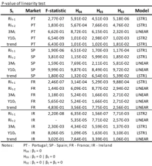
The empirical portion begins with the best linear model for the data (autoregressive model). The lag structure was determined using AIC information criterion. Once the appropriate linear model was defined, we conducted linearity tests against the alternative hypotheses of nonlinearity (STR-type). Table 1 presents these results, which clearly indicate the nonlinearity of the variables (3Mt and Y10t) in Ireland. Only the Y10t variable also maintains nonlinearity in Portugal. The variable 3Mt follows a linear trend in three of the four analysed countries. The variable “trend” is also linear in France and Ireland. For Portugal and Spain, we reject the linearity hypothesis. This finding may indicate the model misspecification of the linear model in that there are parameter changes present that may be captured by LSTR models [see Brüggemann and Riedel (2011), for further details].
Because the main goal of the paper centres on the analysis between adjustments of the available variables, we chose to report the interest rate and stock market returns while considering these variables. The remaining economic variables were not reported. We included one-lagged values of all independent variables and dependent variables in the model.
Table 1. Results of the linearity tests
Therefore, only the Pit-1 was compared in the four countries using a LSTR1 and LSTR2 model. The choice of model was also confirmed, with the highest
P‐value of linearity test
St Market F‐statistic H04 H03 H02 Model
Rit‐1 PT 2,77E‐07 5,91E‐02 4,51E‐03 5,18E‐06 LSTR1
Rit‐2 PT 1,83E‐01 5,67E‐04 7,66E‐01 4,76E‐02 LSTR1
3Mt PT 6,62E‐01 8,72E‐01 6,15E‐01 2,32E‐01 LINEAR
Y10t PT 6,54E‐09 1,01E‐02 2,98E‐07 1,02E‐03 LSTR2
trend PT 6,43E‐03 1,01E‐01 1,02E‐01 1,81E‐02 LSTR1
Rit‐1 SP 1,90E‐06 6,51E‐02 1,70E‐03 1,17E‐04 LSTR1
Rit‐2 SP 3,81E‐02 1,15E‐02 5,99E‐01 1,85E‐02 LSTR1
3Mt SP 1,59E‐01 7,69E‐01 2,11E‐01 5,81E‐02 LINEAR
Y10t SP 9,99E‐01 9,87E‐01 8,49E‐01 9,72E‐02 LINEAR
trend SP 1,80E‐02 1,32E‐02 6,54E‐01 5,39E‐02 LSTR1
Rit‐1 FR 2,46E‐07 3,14E‐04 5,29E‐03 9,88E‐04 LSTR1
Rit‐2 FR 1,44E‐03 6,09E‐01 8,77E‐02 2,94E‐02 LINEAR
3Mt FR 1,18E‐01 5,24E‐01 1,66E‐01 2,71E‐02 LINEAR
Y10t FR 5,65E‐02 5,24E‐01 1,66E‐01 2,71E‐02 LINEAR
trend FR 4,83E‐01 3,56E‐01 7,75E‐01 2,56E‐01 LINEAR
Rit‐1 IR 2,20E‐08 6,35E‐02 1,56E‐07 7,71E‐03 LSTR2
Rit‐2 IR ‐ 5,35E‐05 7,71E‐02 2,57E‐03 LINEAR
3Mt IR 2,30E‐03 4,34E‐02 5,59E‐01 1,37E‐03 LSTR1
Y10t IR 8,06E‐05 1,09E‐05 1,63E‐01 3,10E‐01 LSTR1
trend IR 3,02E‐01 7,64E‐01 3,39E‐01 1,06E‐01 LINEAR
Notes : PT ‐ Portuga l ; SP ‐ Spa i n; FR ‐ Fra nce; IR ‐ Irel a nd H04 : β3 = 0
H03 : β2 = 0 | β3 = 0
p-values in the different countries under study found for the next step in the specification of the STR model, the distinction between logistic and exponential functions. Teräsvirta (1994) suggests testing the following null hypothesis, defined in the note of Table 1.
From the results above, we concluded that in several cases, the linear model fails to model stock returns adequately from macroeconomic variables. This finding led to the next step, which consisted of choosing the appropriate STR model type (k=1 or
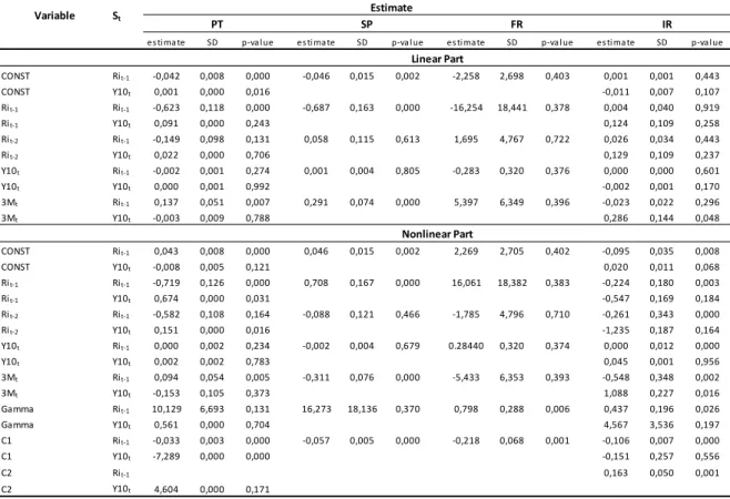
k=2). For example, a LSTR1 model (k=1) describes processes whose dynamic properties differ between periods of expansion and periods of recession, with a smooth transition occurring between the two periods. The LSTR2 model (k=2) is similar at both large and small values of st and different at moderate values [see Teräsvirta (1994) for further references in the STR modelling procedure and application studies]. Table 2. Estimates for STR model
The model specification procedure (Table 1) suggests a single-logistic transition function model when Pit-1 is the transition variable for Portugal, Spain and Ireland. This single transition function infers the existence of two different regimes in these stock markets. Only two cases generate a double transition function: Y10 (Portugal) and Pit-1 (Ireland). The combination of the 3M with Pit-1 in the linear part reveals the significance of the coefficients (Table 2) for Portugal and Spain, whereas the same combination in the nonlinear part was significant for all markets.
An interesting result in Table 2 is the opposite effect that the interest rate variables have in the linear model versus the effects of the same variables during depreciation regimes (registered in Portugal, Spain
and Ireland). Therefore, in the crisis regime, i.e., when there are large negative returns, variable interest rates typically have a large negative impact, which exacerbates the bear market. This situation may partially explain why these three countries were forced to ask for financial assistance from the IMF and the EU.
The estimates of the threshold parameters are important in that they provide information about interest rate levels (in terms of returns, as the data were expressed with reference to returns); in this regard, the nonlinear part of the model becomes relevant. A point of interest is related to the precision of the threshold estimates, which, to judge from the standard errors, are low. In the Portuguese case, where these parameters were higher, this finding may
es tima te SD p‐va l ue es ti ma te SD p‐va l ue es ti ma te SD p‐va l ue es ti ma te SD p‐va l ue
CONST Rit‐1 ‐0,042 0,008 0,000 ‐0,046 0,015 0,002 ‐2,258 2,698 0,403 0,001 0,001 0,443 CONST Y10t 0,001 0,000 0,016 ‐0,011 0,007 0,107 Rit‐1 Rit‐1 ‐0,623 0,118 0,000 ‐0,687 0,163 0,000 ‐16,254 18,441 0,378 0,004 0,040 0,919 Rit‐1 Y10t 0,091 0,000 0,243 0,124 0,109 0,258 Rit‐2 Rit‐1 ‐0,149 0,098 0,131 0,058 0,115 0,613 1,695 4,767 0,722 0,026 0,034 0,443 Rit‐2 Y10t 0,022 0,000 0,706 0,129 0,109 0,237 Y10t Rit‐1 ‐0,002 0,001 0,274 0,001 0,004 0,805 ‐0,283 0,320 0,376 0,000 0,000 0,601 Y10t Y10t 0,000 0,001 0,992 ‐0,002 0,001 0,170 3Mt Rit‐1 0,137 0,051 0,007 0,291 0,074 0,000 5,397 6,349 0,396 ‐0,023 0,022 0,296 3Mt Y10t ‐0,003 0,009 0,788 0,286 0,144 0,048 CONST Rit‐1 0,043 0,008 0,000 0,046 0,015 0,002 2,269 2,705 0,402 ‐0,095 0,035 0,008 CONST Y10t ‐0,008 0,005 0,121 0,020 0,011 0,068 Rit‐1 Rit‐1 ‐0,719 0,126 0,000 0,708 0,167 0,000 16,061 18,382 0,383 ‐0,224 0,180 0,003 Rit‐1 Y10t 0,674 0,000 0,031 ‐0,547 0,169 0,184 Rit‐2 Rit‐1 ‐0,582 0,108 0,164 ‐0,088 0,121 0,466 ‐1,785 4,796 0,710 ‐0,261 0,343 0,000 Rit‐2 Y10t 0,151 0,000 0,016 ‐1,235 0,187 0,164 Y10t Rit‐1 0,000 0,002 0,234 ‐0,002 0,004 0,679 0.28440 0,320 0,374 0,000 0,012 0,000 Y10t Y10t 0,002 0,002 0,783 0,045 0,001 0,956 3Mt Rit‐1 0,094 0,054 0,005 ‐0,311 0,076 0,000 ‐5,433 6,353 0,393 ‐0,548 0,348 0,002 3Mt Y10t ‐0,153 0,105 0,373 1,088 0,227 0,016 Gamma Rit‐1 10,129 6,693 0,131 16,273 18,136 0,370 0,798 0,288 0,006 0,437 0,196 0,026 Gamma Y10t 0,561 0,000 0,704 4,567 3,536 0,197 C1 Rit‐1 ‐0,033 0,003 0,000 ‐0,057 0,005 0,000 ‐0,218 0,068 0,001 ‐0,106 0,007 0,000 C1 Y10t ‐7,289 0,000 0,000 ‐0,151 0,257 0,556 C2 Rit‐1 0,163 0,050 0,001 C2 Y10t 4,604 0,000 0,171 Variable St Estimate PT SP FR IR Linear Part Nonlinear Part
indicate a more substantial nonlinear behavioural adjustment between interest rate and stock market returns. Nonlinearities are associated with the asymmetric effects of threshold adjustment between interest rates and stock market indices.
For Spain, we observed a high standard error for
the γ However, this evidence is not always a signal of
weak nonlinearity: the accurate estimation of the γ parameter is not always feasible, as it requires many observations in the immediate neighbourhood of the threshold parameter c [Teräsvirta, 1998].
From the estimated results for Portugal, two facts may be highlighted. The two regimes correspond roughly to positive and negative values of interest rate growth. The linear and nonlinear components are distinct in terms of the explanatory variables included. All of the variables are presented in both models; however, the signal inverts between them. The standard deviation is higher for the nonlinear component, indicating that the confidence intervals are larger.
The same conclusions may be derived from the Spanish and French markets with the note that the standard error in the Pit-1 variable does not increase in the nonlinear component. The results for the Irish model present the same inversion of signals. However, the Y10t variable is not significant in the nonlinear component.
The LSTR2 models for Portugal and Ireland (with Pit-1 and Y10t as transition variables respectively) both show the signal inversions mentioned before. Furthermore, the Y10t does not appear in the linear component of the Ireland model. The same transition variable is not included in the Portuguese equation, indicating that it has no influence on the model. The estimated coefficients of Portugal tend to be more statistically significant than the other markets in both models (linear and nonlinear).
For all markets, the γ value is slow but always positive, suggesting that the speed of transition between regimes is moderate. The direction of transition is positive for all markets. However for Portugal, Spain and France, the parameter values of β1 are negative. None of the transitions appears to occur abruptly, as the values for estimated γ
parameter for all markets are small. This finding is the same as that obtained by Leybourne et al. (1997). However, it contradicts the results of Patel and Sarkar (1998), stating that prices tend to fall more rapidly and steeply in emerging markets. The threshold parameter c1 for all cases is significant (mostly with a negative value). This finding suggests distinct market behaviour between large negative returns and smaller falls, and positive returns.
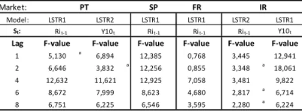
After the nonlinear model estimation, diagnostic tests were performed to evaluate the STR models (Tables 3-6). In particular, we performed misspecification tests for skewness and kurtosis as well as for the ARCH effect of Engle. We also conducted LM tests for autocorrelation, parameter constancy and additive nonlinearity [as suggested by Eitrheim and Teräsvirta (1996)]. The test results indicated no signs of either ARCH or cyclical heteroskedasticity at a significance level of 0.05, nor did they reveal any signs of serial dependence in the estimated residuals.
Table 3. Autocorrelation error Table 4. Remaining nonlinearity
Table 5. ARCH-LM test
No Error Autocorrelation: H0: no
Market: FR
Model: LSTR1 LSTR2 LSTR1 LSTR1 LSTR2 LSTR1
St: Y10t
Lag F‐value F‐value F‐value F‐value F‐value F‐value
1 5,130 a 6,894 12,385 0,768 3,445 12,941 2 6,646 3,832 a 12,256 0,855 3,348 a 18,061 4 12,632 11,621 12,925 7,058 3,481 9,822 6 8,672 7,999 8,623 4,680 2,817 a 6,714 8 6,751 6,225 6,546 3,595 2,280 a 6,224 a Significant at the 5% level. IR PT SP Rit‐1 Y10t Rit‐1 Rit‐1 Rit‐1 No Remaining Nonlinearity: H0: no F F2 F3 F4
PT Rit‐1 1,58E‐04 2,77E‐03 3,00E‐02 2,61E‐02 PT Y10t 5,95E+03 1,90E‐01 4,34E‐02 1,88E‐03 SP Rit‐1 5,81E‐03 7,54E‐01 2,27E‐04 3,78E‐01 FR Rit‐1 6,78E‐02 1,80E‐01 5,68E‐02 3,39E‐01 IR Rit‐1 3,48E‐05 5,37E‐03 1,53E‐02 4,93E‐03 IR Y10t 2,05E‐05 3,44E‐06 9,08E‐02 3,33E‐01
Market: St: F‐Values Parameter Constancy: H0: yes PT SP FR IR Rit‐1 H1 5,879 3,763 2,532a 1,681 Rit‐1 H2 4,016 2,342 1,422 2,567 Rit‐1 H3 3,149 1,883a 1,252 2,068 Y10t H1 1,865 2,961a Y10t H2 1,429 1,665 Y10t H3 1,039 1,736a a Significant at the 5% level. F‐Value T.F. H:
Table 6. Parameter constancy
We failed to find evidence for parameter nonconstancy (Table 6) or evidence for remaining nonlinearity for the full sample. Diagnostic check findings are altered when the transition variable used is the evidence of remaining nonlinearity in several countries. The exception for this case is France, where the Pit-1 does not reflect any evidence of remaining nonlinearity.
For a better understanding of the nonlinear behavioural adjustment, in Figure 1 we present graphs of the transition function in terms of observed values of Δut. Although there is little similarity in the estimated transitions function, there is greater focus when the lagged Pi variable is employed as the transition function (see the cases of Portugal, Spain and France). The logistic function for these markets is centred very close to zero with a steep slope, indicating that the regimes detected by the nonlinear model are related to depreciations, with G(st) = 1, versus appreciations, G(st) = 0. Our findings revealed asymmetric responses of growth to positive and negative Δut, with one linear model applied in periods of depreciation and a different one applied in periods of appreciation. Ehrmann and Fratzscher (2004) also present evidence that the stock market response to monetary policy is highly asymmetric.
From the results we may observe that in cases of asymmetric behaviour, this asymmetry is not around zero returns, as is widely advocated in much of the literature. In line with the results of Reyes et al. (2010), the regime switches are associated with very negative past returns.
It is well known that equity markets react differently to the same news depending on the state of the economy. Bad news always have a positive impact during expansions, and the opposite have a negative impact during recessions. Several studies have found that the financial and banking crises are often related and share common trends. However, in many contexts, especially in recent history, the banking crisis precedes the financial crisis.
Furthermore, the most obvious marker of a potential financial crisis to come in developed countries is a downturn in the equity markets. Stock price movements are more volatile and susceptible than other indicators to several factors.
4.
Conclusion
From our empirical analysis, it is possible to conclude that STR nonlinearities are present in the data, as the linear model fails to model stock market returns. Other highlighted evidence is related to the very strong connections between interest rates and stock markets.
The smooth transition regression approach applied in this study proved to be a viable alternative to the analysis of historical behavioural adjustment between interest rates and stock market indices. This remark is in line with Brüggemann and Riedel (2011), as countries and financial markets react differently to external crises. Combining bonds and stocks from different emerging economies may provide benefits for investment portfolios. [see Kenourgios and Padhi (2012)].
We found evidence in the crisis regime, i.e., large negative returns – interest rate variables typically have a large negative impact, exacerbating the bear market. In the case of Portugal in particular, we obtained the biggest nonlinear threshold adjustment between interest rates and stock market returns. Nonlinearities were associated with the asymmetric effects of threshold adjustment between these two variables. For this market, the linear and nonlinear components were shown to be distinct in terms of the explanatory variables included. Nevertheless, the signal is inverted between the two components.
Finally, the estimated models highlight the importance of modelling the cyclical behaviour of stock market returns to identify the real significance of the influence of interest rates on returns. Nonlinear threshold adjustment between bond markets and stock markets has implications for an investment strategy based on only one of these markets. It appears that any potential benefits from international diversification are greater for bond investors than for stock investors. Aslanidis and Christiansen (2012) have explored the similar effects of large short rates on the present value of future stock and bond returns, thereby implying a positive stock-bond correlation. In this context, investors flee stocks and rush into bonds [flight to safety]. This movement implies negative
St: Statistics: PT SP FR IR
Rit‐1 Test : 155,293 67,995 127,849 164,610
Y10t Test: 153,053 211,286
Rit‐1 F: 23,278 9,166 18,512 24,973
stock-bond correlations. The authors conclude that this flight in times of high levels of uncertainty explains why the stock-bond correlations become negative.
Further detailed analysis should be made to clearly identify the alarm signals to prevent an imminent market crisis.
References
[1] Aslanidis, N., Christiansen, C., 2012. Smooth transition patterns in the realized stock-bond correlation. J. Empirical Finance, 19, 454-464. [2] Brüggemann, R. Riedel, J., 2011. Nonlinear
interest rate reaction fuctions for the UK. Econ. Model., 28, 1174-1185.
[3] Calvo, G.A., Izquierdo, A., Mejía, L.-F., 2004. On the empirics of sudden stops: the relevance of balance-sheet effects. NBER Working Paper 10520.
[4] van Dijk, D., Terasvirta, T., Franses, P.H., 2002. Smooth Transition Autoregressive Models – A Survey of Recent Developments. Econometrics Rev., 21, 1-47.
[5] Chan, K.S. Tong, H., 1986. On estimating thresholds in autoregressive models. J. Time Ser. Anal., 7, 179-90.
[6] Ehrmann, M., Fratzscher, M., 2004. Equal size, equal role? Interest rate interdependence between the Euro area and the United States. ECB Working Paper 342.
[7] Eitrheim, Ø, Teräsvirta, T., 1996. Testing the adequacy of smooth transition autoregressive models. J. Econometrics, 74, 59-75.
[8] Granger, C., Teräsvirta, T., 1993. Modelling Nonlinear Economic Relationships. Oxford University Press.
[9] Kenourgios, D., Padhi, S., 2012. Emerging markets and financial crises: Regional, global or isolated shocks? J. Multinatl. Financ., 22, 24-38.
[10] Leybourne, S.J., Sapsford, D.R., Greenway, D., 1997. Modelling Growth (and liberalisation) using Smooth Transitions. Anal. Eco. Inquiry, 35, 798-814.
[11] Neumeyer P.A., Perri, F., 2005. Business cycles in emerging economies: the role of interest rates. J. Monetary Econ., 52, 345-380.
[12] Patel, S. Sarkar, A., 1998. Stock market crises in developed and emerging markets. Research Paper 8909, Federal Reserve Bank of New York.
[13] Reinhart, C., 2002. Sovereign debt ratings before and after financial crises. MPRA Paper 7410. University Library of Munich.
[14] Reyes, C., Alellie, S. Jeremy, J., 2010. The Impact of the global financial crisis on poverty in the Philippines. PIDS Discussion Paper 04. Philippine Institute for Development Studies. [15] Teräsvirta, T., 1998. Modeling economic
relationships with smooth transition
regressions, in: Ullah, A. and Giles, D. (Eds.), Handbook of Applied Economic Statistics, Dekker, New York, pp. 507-552.
[16] Teräsvirta, T., 1994. Specification, estimation, and evalution of smooth transition
autoregressive models, J. Am. Stat. Assoc., 89, 208-218.