M
ESTRADO
F
INANCE
T
RABALHO
F
INAL DE
M
ESTRADO
PROJECTO
CREDIT DEFAULT SWAPS
–
BROKEN BASIS AND COUNTERPARTY
RISK
M
ESTRADO EM
F
INANCE
T
RABALHO
F
INAL DE
M
ESTRADO
PROJECTO
CREDIT DEFAULT SWAPS
–
BROKEN BASIS AND COUNTERPARTY
RISK
RICARDO FILIPE GODINHO MIRANDA DAS NEVES
O
RIENTAÇÃO
:
P
ROFESSORA
R
AQUEL
M.
G
ASPAR
Abstract
This study aims to analyse whether periods of financial turmoil caused the relation between CDS and corporate bond spreads (CDS-Bond basis) to structurally break. We obtained evidence that a higher number of breaks were detected during the European sovereign debt crisis for the firms included in the sample. Besides, firm specific coun-terparty risk effect on the basis revealed also to have stronger impact on financial firms in the after-break period.
Resumo
Este estudo pretende analisar se per´ıodos de turbul ˆencia nos mercados financeiros causaram uma quebra de estrutura na relac¸ ˜ao entre os spreads dos CDS e das Obrigac¸ ˜oes (Base). Obtiv ´emos evid ˆencia que um largo n ´umero de quebras de estrutura foi detec-tado para as empresas inclu´ıdas na amostra durante o per´ıodo da crise da d´ıvida soberana Europeia. Para al ´em disso, o efeito do risco de contra parte na base revelou ter tamb ´em um maior impacto nas empresas do sector financeiro no per´ıodo ap ´os a quebra de estrutura detectada.
1
Acknowledgments
Beforehand, i would like to thank my supervisor Raquel Gaspar for all
the advices given along the process and for her critical and constructive
spirit, particularly in the tough stages. I am also grateful to my colleagues
that accompanied me in the brainstorming sessions and to my parents that
List of Abbreviations
CDS-Credit Default Swaps
Basis- CDS-Bond Basis
ECB- European Central Bank
ZA- Zivot and Andrews
US- United States of America
CCP- Central Clearing Counterparty
AIG- American Insurance Group
ADF- Augmented Dickey-Fuller
List of Tables
1 Yield spread computation for ELEPOR 6.4 10/29/2009 Corp 8
2 Descriptive Statistics . . . 11
3 Dataset Description . . . 33
4 Primary Dealers List . . . 34
5 ZA Test: CDS Levels . . . 35
6 ZA test: ∆(CDS) . . . 36
7 ZA Test: Bond spreads . . . 37
8 ZA test: ∆(Bondspread) . . . 38
9 Cointegration Results with Structural Break . . . 39
10 Bai and Perron (2003) Detected Structural Breaks . . . 40
12 Time Series Determinants of CDS-Bond Basis: Multivariate
Regressions - Non Financial . . . 42
List of Figures
1 CDS premiums . . . 92 CDS-Bond basis evolution . . . 10
3 VSTOXX evolution . . . 23
4 Euribor 3 Month - EONIA Spread . . . 24
Contents
1 Acknowledgments i
2 Introduction 1
3 Theoretical Framework 3
4 Methodology 5
4.1 Data . . . 5
4.2 CDS-Bond Basis . . . 6
4.3 Long-Term Relationship Between CDS and Bond Spreads . 13 4.3.1 Unit Root Tests . . . 13
4.3.2 Cointegration Tests . . . 15
4.3.3 Structural Break Detection . . . 18
4.4 The Determinants Of Basis Spread Changes . . . 19
4.4.1 Liquidity Factors and Market Volatility . . . 22
4.4.2 Counterparty Risk . . . 23
5 Analysis of the Results 28 5.1 Long-Run Movement . . . 28
5.2 CDS-Bond Basis Structural Breaks . . . 29
5.3 Multivariate Regressions . . . 29
6 Conclusion and Future Research 30
2
Introduction
During the past decades, several innovative credit derivatives began
trading in financial markets. Among those structured products, credit
de-fault swaps (CDS) took particular attention. A CDS acts like an insurance
agreement between two parties, where the protection buyer pays a
peri-odic fee (CDS spread) to the seller until the contract matures/expires or
the reference entity’s is subject to a credit event. In case a credit event
oc-curs within/during the contract’s time frame, two settlement methods are
possible. First, a physical settlement where the buyer transfers the
refer-ence entity’s bond and gets in return from the seller the bond’s full face
value. The alternative method builds on cash settlement where the seller
pays the difference between face value and the bond recovery value. In
this case an auction gets in place in order to reach this recovery rate and
the consequent contract settlement.1 According to the trade organization
that guarantees the operability of the CDS market ISDA, a credit event for
European corporate contracts occur in the presence of bankruptcy, failure
to pay(default) or restructuring.
Besides hedging against a reference entitys default, CDS spreads can
also provide an important continuous assessment of an entity’s credit
con-ditions. Increasing (decreasing) spreads should reflect deteriorating
(im-proving) credit conditions and higher probability of default. CDS contracts
are traded bilaterally in over-the-counter (OTC) markets negotiated
pri-vately between dealers and investors.
1For a more detailed explanation regarding the auction process, see Coudert and
In the last quarter of 2008, AIG had to be bailed out by the US
gov-ernment due to their huge exposure on CDS as protection seller. The
interconnectivity and lack of transparency of trades in OTC markets
com-bined with AIG potential default could severely increase the risk of collapse
in the financial system. This event as well as the subprime crisis in general,
first alerted investors, regulators and supervisors for the potential dangers
of counterparty risk in the CDS market.
In a simplistic way, CDS and bonds can be considered to reflect the
same type of risk: inability of an entity to meet the required payments on
its debt obligations. Several authors such as Duffie(1999) argue that both
CDS premiums and corporate yield spreads share a theoretical
equilib-rium condition. This relation between these two markets is known as the
CDS-Bond basis, henceforth mentioned just as basis.
The aim of this study is to assess the impact periods of financial
insta-bility had on the evolution of both CDS and bond markets. While previous
studies focused primarily on the subprime crisis, this analysis contributes
by also extending and including the more recent European sovereign debt
crisis period. For that purpose, first we identify whether certain dates
caused the CDS-Bond basis relation to structurally change. Then, the
main point is to check for the possibility of relating those detected break
dates to major events that occurred in the recent financial crisis such as
the Lehman Brothers collapse in 2008 or the Greece government bail
out in 2011. Lastly, explanatory power of several determinants that
in-fluence CDS-Bond basis dynamics is compared before and after the
en-dogenously detected structural date in order to measure if risks began to
The remainder of this text proceeds as follows.In Section 3 is
pre-sented theoretical guidance regarding some main concepts to be applied
throughout the study. Section 4 describes both dataset and methodology
employed in basis construction and subsequent analysis regarding
station-arity, cointegration, structural break detection and determinants of basis
dynamics. Presentation and analysis of the results is discussed in Section
5. Section 6 concludes and presents suggestions for future research.
3
Theoretical Framework
Before proceeding to the analysis of the CDS-Bond basis, it is
use-ful to provide theoretical guidance regarding some concepts to be applied
in this study. In theory, CDS and bonds are two different securities
ex-posed to the same type of risk: inability of entity’s to meet the required
payments on their debt obligations. Intuitively, if an investor is long on a
par yield bond and simultaneously enters a Credit default swap contract as
protection buyer, in principle the default risk exposure over that reference
entity is eliminated.2 Therefore, this theoretical equilibrium condition
be-tween CDS and bond spreads known as the CDS-Bond basis should be
observed.3 Formally:
CDS Bond Basist =CDSt−(yt−yrf)(1)
Whereytandyrf correspond respectively to the entity’s bond yield and
the benchmark risk free rate. Although the relationship between these two
2This portfolio strategy should provide the investor with a return equal to the yield of a
risk-less security such as the Treasury Rate for example.
market segments should on average hold, authors document that during
turbulent periods characterized by financial instability the basis deviates
from parity. If perfect capital markets existed, investors could then exploit
a theoretical arbitrage opportunity. If the basis turns negative, investors
could benefit from buying the bond (higher yield makes it cheaper) and
consequently buying protection through CDS contract.4 Fontana (2010)
documents that during the subprime crisis, counterparty risk and
increas-ing fundincreas-ing liquidity shortage made it much more expensive to trade a
persistently negative basis. Bai and Dufresne(2011) report that instead of
a clear factor, several drivers particularly the risk of counterparty default
and investors investments transfer to less risky and more liquid securities
such as Treasury bills (flight to quality risk), dropped the CDS-Bond basis.
CDS and Bonds cannot be seen as perfect substitutes since they are
exposed to different types of risk others than credit risk, such as
coun-terparty risk. This type of risk lowers CDS premiums as dealers and
in-vestors could fail to meet their obligations and so are willing to pay a lower
spread(Wit 2006).
In time series analysis, valid statistic inferences can only be made if
variables have constant long-run mean and finite variance across
obser-vations i.e. are considered stationary. Otherwise, series is said to contain
a unit root process and their use leads to a spurious regression as usual
statistical inferences do not hold. Time series are considered to follow a
unit root process if the value of the series in one period equals its previous
period plus an unpredictable error. In case a time series appear to have a
unit root, a successful method often relies on first difference in levels i.e.
I(1).
4Inversely, investors should short sell the corporate bond and sell protection through
However even if variables alone follow a unit root process, in the long-run
they may share a linear combination. In that case, CDS and bond spreads
are said to be cointegrated and therefore regressing involving their
lev-els can proceed without generating spurious results (Engle and Granger
1987).
Recent empirical studies such as Perron (2005), alert for the
similari-ties and interconnectivity between non-stationarity and structural changes.
This topic brings questions whether do CDS follow a stationary process
with the impact of a structural break somewhere along the time series
rather than containing a unit rooting in the presence of market instability
such as the collapse of Lehman Brothers for examples.
A structural break is stated to occur when at least one parameter in the
model has shifted permanently at some point in the time series. (Hansen
2001). The point in time where that parameter change occurs in the model
is termed as ”break date”.
4
Methodology
4.1
Data
The analysis comprises the period from March 2007 until March 2014.
For that purpose, daily 5-year credit default swap quotes were retrieved
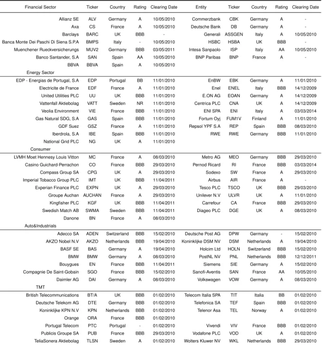
from a Bloomberg financial terminal5. The sample consists of 74 investment-grade firms included in ITraxx Europe, a CDS index for the most liquid
European companies. In Table 1 it is possible to observe the full dataset
description divided by ratings, tickers and sector of activity.
4.2
CDS-Bond Basis
The CDS-Bond Basis enables investors to assess the perceived
en-titys default risk condition in two different markets by comparing its CDS
spread with the corporate yield premium relative to a benchmark risk free
rate. However, its computation is tied to two important issues. The first
is-sue lies in the choice of the riskless benchmark for corporate bond spread
computation. Nowadays, the common reference rate used by authors as
risk-free benchmark is the interest rate swap curve, I-Spread, over the
tra-ditional Treasury rate. Unlike government bond yields that suffer from tax
advantages, scarcity premium and repo specialness (Blanco et al. 2005),
interest rate swaps benefit from being quoted on constant maturity basis
and seen as a better approximate funding cost to investors. Nevertheless,
since the analysis will take higher emphasis on counterparty risk impact
on basis changes, European Central Bank (ECB) spot yield curve will be
used as proxy riskless benchmark as swaps carry an amount (although
small) of counterparty and default risk due to its floating leg being indexed
to Euribor.
Thus the next step would be calculating the basis by comparing the
CDS spread with the correspondent 5-year maturity bond. Yet, it often
proves a difficult task to find bonds that exactly match CDS contracts
con-stant maturity. So, in order to overcome this maturity matching problem,
literature suggest three different ways. The first approach falls on the
par-equivalent spread methodology, where the fair value of CDS is compared
to market bond spread based on CDS-implied default probabilities (Elisade
et al. 2009 and Bai and Dufresne 2011). Alternatively, Blanco et al. (2005)
ma-turity above and below the desired. Then, they linearly interpolate those
yields in order to estimate the desired constant risk free yield to maturity.
However, this study will follow the methodology presented in Longstaff
et al.(2005). Their methodology builds on the following procedures: (1) a
set of bonds is first selected to bracket the desired maturity. Their bond
sample consists of only fixed coupon rate, large issues of senior debt
obli-gations and excludes any that contain embedded option such as
cheapest-to-deliver (CTD) or convertible bonds6(2) Then, a riskless bond is created
with the same coupon rate and maturity as the risky one using the
pro-vided daily ECB yield curve parameters as benchmark. For that purpose,
daily discount factorsy, are computed using the Nelson-Siegel-Svensson
model (SSN):
y(n) =β0+β1
1−e −
n λ1 ! n λ1
+β2
1−e −
n λ1
!
n λ1
−e −
n λ1 !
+β3
1−e −
n λ2
!
n λ2
−e −
n λ2 ! (2)
The advantage of the Svensson model is that there is no need for
in-terpolation since the estimation is adjustable for the desired maturity. After
calculating the corporate yield spread for each bond included in the
bas-ket, the next step is to regress the spreads on their maturities and then
use the predicted value at 5-year as the observation date bond spread.
The CDS-Bond basis is then obtained by the difference of CDS premium
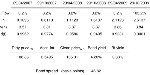
relative to the regressed corporate yield spread. In Table 1 is presented an
illustrative example for the energy sector firm Energias de Portugal (EDP),
6Authors present in Appendix B of their paper full criteria for the choice of bonds to be
regarding a risk-less yield computation on 20thMarch 2007 for a bond that
pays semi-annual coupons.
Table 1 Yield spread computation for ELEPOR 6.4 10/29/2009 Corp
29/04/2007 29/10/2007 29/04/2008 29/10/2008 29/04/2009 29/10/2009
C.Flow 3.2% 3.2% 3.2% 3.2% 3.2% 103.2%
n 0.1096 0.6110 1.1123 1.6137 2.1123 2.6137
y(n) 3.57 3.81 3.87 3.87 3.86 3.84
d(t) 0.9962 0.9774 0.9586 0.9405 0.9231 0.9061
Dirty priceRf Accr. Int Clean priceRf Bond yield Rf yield
108.86 2.5495 106.31 4.20% 3.83%
Bond spread (basis points) 46.82
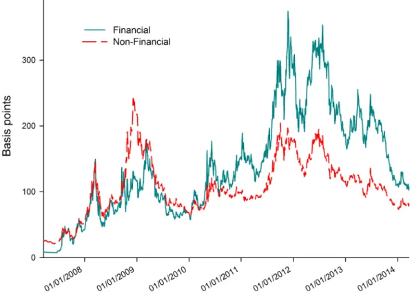
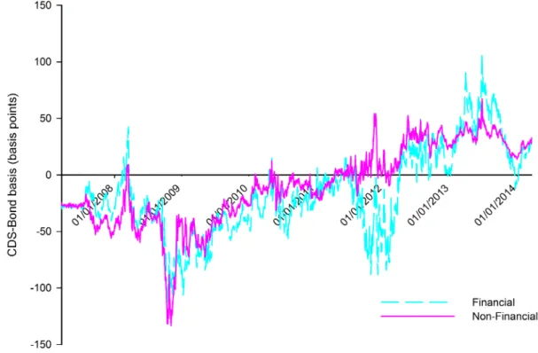
Applying the methodology described previously to the remaining firms
of the sample, Figure 1 and Figure 2 represent respectively the average
CDS spreads and CDS-Bond basis evolution during the covered period for
Figure 2 CDS-Bond basis evolution
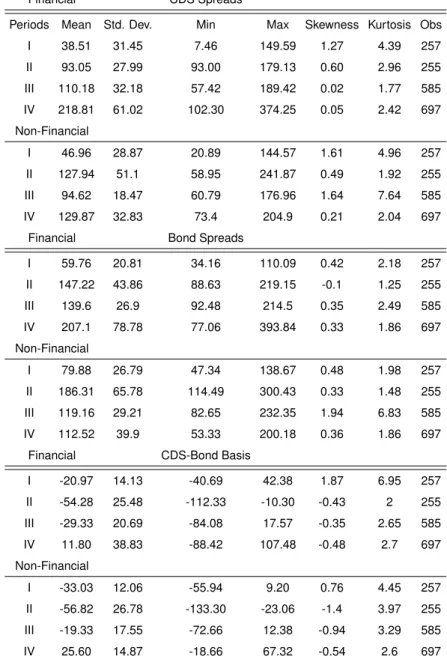
Descriptive statistics regarding the CDS premiums, bond spreads and
the correspondent CDS-Bond basis are presented in Table 2. The
time-line addressed in the analysis will be divided in four different periods to
compare the evolution of the variables in question. Once again, distinction
will be made between financial and non financial firms. The first period
will include the pre-subprime crisis until the acquisition of Bear Sterns by
JPMorgan Chase in March 2008. The next period comprises the
finan-cial turmoil characterized by the collapse of Lehman Brothers until March
2009, wherein markets began to stabilize. Thereafter, up to July 2011
fol-lowing the changes implemented in the CDS market through the Big Bang
Table 2 Descriptive Statistics
Financial CDS Spreads
Periods Mean Std. Dev. Min Max Skewness Kurtosis Obs I 38.51 31.45 7.46 149.59 1.27 4.39 257 II 93.05 27.99 93.00 179.13 0.60 2.96 255 III 110.18 32.18 57.42 189.42 0.02 1.77 585 IV 218.81 61.02 102.30 374.25 0.05 2.42 697 Non-Financial
I 46.96 28.87 20.89 144.57 1.61 4.96 257 II 127.94 51.1 58.95 241.87 0.49 1.92 255 III 94.62 18.47 60.79 176.96 1.64 7.64 585 IV 129.87 32.83 73.4 204.9 0.21 2.04 697
Financial Bond Spreads
I 59.76 20.81 34.16 110.09 0.42 2.18 257 II 147.22 43.86 88.63 219.15 -0.1 1.25 255 III 139.6 26.9 92.48 214.5 0.35 2.49 585 IV 207.1 78.78 77.06 393.84 0.33 1.86 697 Non-Financial
I 79.88 26.79 47.34 138.67 0.48 1.98 257 II 186.31 65.78 114.49 300.43 0.33 1.48 255 III 119.16 29.21 82.65 232.35 1.94 6.83 585 IV 112.52 39.9 53.33 200.18 0.36 1.86 697
Financial CDS-Bond Basis
I -20.97 14.13 -40.69 42.38 1.87 6.95 257 II -54.28 25.48 -112.33 -10.30 -0.43 2 255 III -29.33 20.69 -84.08 17.57 -0.35 2.65 585 IV 11.80 38.83 -88.42 107.48 -0.48 2.7 697 Non-Financial
I -33.03 12.06 -55.94 9.20 0.76 4.45 257 II -56.82 26.78 -133.30 -23.06 -1.4 3.97 255 III -19.33 17.55 -72.66 12.38 -0.94 3.29 585 IV 25.60 14.87 -18.66 67.32 -0.54 2.6 697
Relative to average CDS premiums, period I exhibits the lowest value
during the period covered. Despite being characterised as the tranquil
pe-riod, a negative CDS-Bond basis of -20 basis points is observed which
bond). A possible explanation for this behaviour could be related with
liq-uidity issues in the choice of the ECB yield curve for riskless benchmark
as mentioned previously, such as tax advantages or scarcity premium. Up
to this point, different sectors follow the same evolution pattern. Yet, it is
during financial crisis that we observe differences on cross-sectional
be-haviour.
During the sub-prime crisis, CDS spreads increased and the average
basis fell to -133 basis points for financial firms and -112 to non-financial.
This behaviour is somewhat surprising as it contrasts with other studies
such as Fontana(2010) and Augustin(2012), where the basis went down
in a more dramatically way, particularly for financial firms. In their case,
they reported an average negative basis of 145 basis points.
Neverthe-less, their studies are based on the US financial sector where the financial
turmoil was originated, so in theory a stronger impact was expected there,
at least in the short term. With the exception of the first period in analysis,
the variables present negative skewness and excess kurtosis.
In period III is observed the stabilization of market conditions. While in
the industry sector is seen a reduction, financial firms suffer from spread
enlargement. It was also by that time that significant changes were
imple-mented on the CDS market, such as Clearing House implementation. In
Period IV following European sovereign debt crisis and major events
con-cerning financial assistance programs to Portugal, Spain and Greece the
inverse situation is observed, being the financial sector more affected than
non-financial firms, particularly driven by financing issues. In 2012 with
pay-ments through Greece default in March of that year, premiums
enlarge-ment can be observed specially for the financial sector, where spreads
reached higher values than during 2008 financial crisis (over 300 basis
points). With the ban of naked sovereign CDS in 2012, investors began
to hedge their risks by shifting their investment to financial companies.
Allied with the difficulty in financing themselves, credit risk perception by
investors increased and consequently CDS premiums.
4.3
Long-Term Relationship Between CDS and Bond Spreads
4.3.1 Unit Root Tests
Previous studies proved that in most cases CDS and bond spreads
do not follow a stationary process, either by applying Augmented
Dickey-Fuller(ADF) or KPSS test to check for that condition.
Nevertheless, recent empirical studies alerted for the similarities and
interconnectivity between a unit root process and the occurrence of a
break at a given time in the sample. As addressed by Perron (1989),
failure to reject the hypothesis of a unit root process could be misleading
as it could rather imply the presence of a structural break in the series.
Different from Nelson and Plosser (1982), the author states that instead of
unit root, time series may follow a stationary process around a trend
func-tion allowing for a large infrequent shock at some point in their intercept
and slope. For that purpose, a modified ADF test was proposed,
includ-ing a time dummy variable in the regression for the presence of a break
under both the null and alternative hypothesis. Yet, this method presents
exoge-nous break. So, in order to overcome the limitation described, Zivot and
Andrews (1992), Lumsdaine and Papell (1998), Lee and Strazicich (2003)
among others, developed unit root tests to endogenously detect a
struc-tural break, indicating that this way, the bias related to usual tests could be
reduced.
Therefore, since the period in analysis comprises at least two major
events, the 2008 subprime crisis and the 2010 sovereign debt crisis, a unit
root process in the presence of structural break should also be tested. For
that purpose, tests suggested by Zivot and Andrews (1992) are applied.
Zivot and Andrews test proceed as follows: First, for every observation
date in the sample a dummy variable is created and regressed
sequen-tially using the ADF test. Then, amongst all the selected potential break
dates (TB), the one which minimizes the t-statistic of the unit root test is
the selected as a break in the time series. The null hypothesis of unit root
versus a one-time endogenously detected structural break wherey
repre-sents the variable tested, can be applied through three different models:
yt =c+αt−1+β∗t+γ∗DUt+
Pk
j=1dj yt−j +εt
yt =c+αt−1+β∗t+θ∗DTt+
Pk
j=1dj yt−j +εt
yt =c+αt−1+β∗t+θ∗DUt+γ∗DTt+
Pk
j=1dj yt−j +εt
(3)
While model A allows for a one-time level shift in the time series, Model
B checks for a one-time slope change. . On the other hand, model C
in-corporates both mean and trend shift where DUt and DTt account for a
break occurrence in the mean and trend respectively. The next question
appear to exhibit a deterministic trend, unit root analysis is made to
ac-count for both a change in the intercept and slope (model C). Otherwise,
only a break in the intercept through model A is analysed.7 Firms that in
their levels refuted the null hypothesis in both CDS and bond spreads will
be treated from now on as I(1), as they proved to be stationary in their
first-differences.
4.3.2 Cointegration Tests
As mentioned before, regressing non-stationary variables may lead to
spurious regressions and their economic interpretation will not be
mean-ingful. Nevertheless, if the linear combination between two non-stationary
variables happens to be stationary, they are said to possess a long-run
equilibrium condition i.e. cointegrated. That way, while variables may
de-viate from each other on the short term, ultimately they will mean revert.
If cointegration is found on CDS and bond spreads, that is, non stationary
variables follow a long-run relationship, regression can be applied without
generating spurious results.
Several authors like Fontana (2010), and Blanco and Brennan (2005),
applied the Johansen (1988, 1991) procedure to assess the long-run
equi-librium between CDS and bond spreads. Nevertheless, the Johansen
test is better fit to analyse multivariate time series which test for
multi-ple cointegrating ranks. So, Wit (2006) and Gaspar and Fonseca (2011)
simpler approach is then employed through the Engle and Granger (1987)
methodology.8 First, residuals are OLS estimated by regressing CDS on
bond spreads. Then, predicted residuals stationarity is tested through the
standard ADF test. When that condition is observed, errors variance is
time-invariant and variables are considered to move together in the long
run. That way, OLS regressing first difference cointegrated variables does
not lead any more to misleading inferences.
However these findings are only indicative since long-run equilibrium
condition between two markets allowing for a possible structural change
cannot be tested through Engle and Granger method, such as Lehman
Brothers for example.Therefore, we apply the Gregory and Hansen (1996)
approach, where a single unknown structural change in the cointegrating
relationship is tested under the alternative hypothesis. The authors argue
that instead of thinking in a time invariant relationship between variables,
cointegration could hold for some period of time, and then shifting to a new
“long-run” equilibrium after the occurrence of a break in the time series. In
order to account for a possible structural change, a dummy variable is
in-corporated in the regression:
ϕt=
0, ift ≤[n∗τ]
1, ift >[n∗τ]
Where the unknown parameterτ ∈(0, 1) denoted the relative timing of
the change point and [ ] denotes the integral part (Gregory Hansen 1996).
This approach allows the testing of one structural change through the three
forms:
Bond Spreadt=µ1+µ2ϕtτ +t+εt
Bond Spreadt=µ1+µ2ϕtτ +βt+t+εt
Bond Spreadt=µ1+µ2ϕtτ +α1CDSt+α2CDStϕtτ +εt
(4)
The first model tests for cointegration in the presence of a level shift in
the time series (C), where µ1 and µ2 represent respectively the intercept
before the break and the change in the intercept at the time of the level
shift. Similar to the first model, model 2 tests for a constant shift while
introducing a trend vector in the regression as well (C/T). In this case,
βt is the trend slope before the break and at the slope coefficient which
is assumed to be constant. Under model 3, the cointegrating vector is
allowed to both slope and shift parallel which is mentioned by authors as
the regime shift model. The slope coefficient changes are represented in
the α2t variable whileα1t denotes the coefficients before the shift. Similar
to Engle and Granger (1996), residuals are OLS regressed and then unit
root tests are applied to the estimates. Then, both ADF and Philips-Perron
Za andZt tests are sequentially employed across the break points, where
the one that contains the smallest value (largest negative) is presented.
For that break date, if the test statistic is lower than critical value, there is
evidence of cointegration between the variables.
4.3.3 Structural Break Detection
In previous sections, testing for cointegration between CDS and bond
market or for a stationary process were checked allowing for the
occur-rence of a single structural break in the time series. However, assuming
that the CDS-Bond basis presents only one structural change during the
comprised period could be misleading, particularly since it comprises
European sovereign debt crisis. Therefore, it is proposed to test for the
existence of multiple structural breaks in the CDS-Bond basis during the
covered period.
Regarding this subject, an earlier method was presented by Garcia
and Perron (1996) testing for the presence of two regime shifts in the US
real interest rate through the sup-Wald test. The drawback behind their
approach is again the limited number of structural breaks allowed.
In order to overcome the mentioned limitation, endogenously detected
multiple structural change tests are applied through Bai and Perron (1998,
2003) methodology. The process allows to detect up to five break points
and is disentangled in two different parts. First, a number of breaks
lim-ited to an upper bound (m) previously chosen are estimated based on the
least squares principle (global optimization). Then, the breaks statistical
significance using asymptotical critical values is tested through: (1) sup
F type test where is tested the hypothesis of zero versus less or equal to
m structural changes, (2) double maximum tests, UDmax and WDmax,
where the null hypothesis of no structural breaks is tested againstm
struc-tural changes and (3) sequential test sup Ft(l+1/l), for null hypothesis of
l versus l+1 structural breaks. The optimal number of breaks is detected
when the null hypothesis can no longer be rejected, that is, the critical
value exceeds the test statistic. As suggested by Perron (2005), double
maximum tests are first used in order to ascertain if any break is present.9
In that case, break dates are then estimated through the sequential test
9The procedure of Bai and Perron (2003) also corrects for serial correlation and
supFt(l+1/l) test until it fails to reject the null hypothesis.10
4.4
The Determinants Of Basis Spread Changes
This section concludes by describing the main basis drivers used in
literature and then present the ones to be applied in the study. According
to several authors, namely Colin-Dufresne, Goldstein, et al. (2001),
Eric-sson, Jacobs and Oviedo (2009) among others, determinants like a firms
leverage or market implied volatility increase and contain high explanatory
power in explaining default risk. Hull, Pedrescu and White (2004) argue
that credit rating downgrades lead in half of the cases CDS spreads and
that negative correlation exists between them. On the other hand, authors
document that positive credit rating events impact were less significant.
Blanco, Brennan et al.(2005) relied especially on market variables to
analyse basis dynamics such as Stoxx indices implied volatility or the
changes between 10- and 2-year treasury bonds to capture the slope of
the yield curve. They concluded that the theoretical no arbitrage relation
between CDS and bond spreads held for most firms included in their
sam-ple. Yet, for some European companies that was not the case, probably
due to the cheapest-to-deliver option incorporated in some CDS contracts.
Since the protection buyer delivers the most favourable (cheapest) bond in
case of a credit event, the seller will require a higher premium to
compen-sate for that risk which consequently increases the basis (Wit 2006).
Longstaff (2005) approach differentiates between default and non-default
10Only the break dates will be presented in order to save space, but the statistics are
components when comparing CDS spreads to corporate yield spreads.
The author states that default risk is predominantly priced in yield spreads,
increasing particularly for speculative grade firms. Nevertheless,
non-default factors such as corporate bond illiquidity are still significant at
ex-plaining credit spread changes, particularly bonds maturity, notional amount
outstanding and bid-ask spreads. On the other hand, special treatment
re-garding tax asymmetry relative to Treasury over corporate bonds since the
latter are not exempt, proved less significant.
Similar to Blanco et al. (2005), Zhu (2006) states that the equilibrium
condition between CDS and tend to move together on the long-run i.e. are
cointegrated, while in the short-term this no-arbitrage premise does not
hold. For that purpose, the author provides several determinants to model
the basis dynamics in panel organised data. They include equity indices
as market conditions but also firm specific variables, such as lagged basis
changes or incorporation of dummy variables relative to rating events,
cur-rency denomination, credit type and restructuring clause11. Besides, CDS
aggregate number as well as bond bid-ask spreads are meant to infer the
evolution of the firms liquidity condition.
With the advent of the financial crisis in 2008, several authors present
a persistent negative basis during that period, namely Augustin (2012),
Bai-Dufresne (2011), among others. As mentioned previously, before the
financial turmoil literature focus fell particularly on default and liquidity risk
in credit spreads. However, the persistent negative CDS-Bond basis
dur-ing financial turmoil brought the attention of counterparty risk to the
thors.
Fontana (2010) and Bai-Dufresne (2011) argue that no single factor
can be appointed as the cause of breaking the no-arbitrage condition
be-tween CDS and markets but rather a set of drivers, namely funding,
coun-terparty risk and collateral quality. Both authors emphasized the
fund-ing liquidity shortage and increase of counterparty risk durfund-ing that period,
through the Libor-OIS spread. The Libor-OIS spread should reflect the
risk premium related to inter-bank lending and a higher gap increases the
likelihood of counterparty default since lending conditions get severed
be-tween systemically important firms.
Therefore, this explanatory variable has a negative effect on the
CDS-bond basis since a CDS buyer will be willing to pay less for protection if
the counterparty probability to default increases. Augustin (2012) argues
that during the subprime crisis, the basis dropped significantly less for the
financial sector relatively to non-financial firms. The author argues that
fi-nancial firms, particularly banks, were considered by governments as
sys-temically important and often seen astoo big to fail. Nevertheless, Lehman
Brothers collapse could have changed that view and investors rushed to
get protection on those firms which consequently increased CDS spreads
and consequently the basis. In order to reach this conclusion, dummies
were applied to differentiate between periods and sectors of activity.
Based upon the literature regarding determinants of basis changes, the
4.4.1 Liquidity Factors and Market Volatility
Following Longstaff (2005) and Fontana (2010), CDS and bonds
bid-ask spread (BAS) will be applied in order to assess how liquidity influences
the basis dynamics during the period covered. Quotes for bid and ask CDS
5-year tenor were retrieved from Bloomberg financial terminal. Then, the
spread is simply computed as the difference between ask and bid
quo-tation. Regarding bond spreads, as we face the same maturity
match-ing problem mentioned previously, the same procedure when computmatch-ing
the CDS-Bond basis is applied. For every bond included in the basket of
bonds, the bid-ask spread is calculated and then regressed on their
matu-rities to obtain the constant 5-year tenor.(Gaspar and Fonseca 2011)
Following the advices from Oviedo (2009), Zhang, Zhou and Zhu (2009),
Blanco et al. (2005), among others, VSTOXX,a volatility index based on
Euro Stoxx 50 option meant to measure the overall European market
long-term volatility is also included in the analysis. Figure 3 reports the index
Figure 3 VSTOXX evolution
4.4.2 Counterparty Risk
In order to account for the fact a counterparty at some point may fail to
meet its obligations in case of a credit event, three proxies are employed
in the analysis: (A) the Euribor-EONIA spread (equivalent to LIBOR-OIS
for Europe) as stated by Fontana (2010), is an indicator of both funding
liquidity and counterparty risk in the context of inter banking lending12.
Therefore, increasing spread is associated with lender’s belief that the risk
of default on interbank loans is higher. Figure 4 presents the evolution of
the Euribor - EONIA spread:
Figure 4 Euribor 3 Month - EONIA Spread
Beginning in the second half of 2007, Euribor-EONIA spread became
rather unstable with large fluctuations, particularly with Lehman Brothers
collapse in September 2008, where the spread increased to nearly 200
basis points in 10 trading days. Then in 2009, markets and consequently
credit conditions began to stabilize until the fear of a Greek sovereign
de-fault in 2011 led again to a gap widening, reaching the 100 basis points.
(B) The second proxy for counterparty risk follows the approach
an equally weighted index constituted by the primary dealers in the CDS
market. The introduction of central clearing counterparties (CCP) in meant
to standardize the market and reduce counterparty risk to minimal
lev-els as CCP is responsible for every contracts settlement. Therefore, ICE
Clear Europe member’s can be considered to reflect the major dealers in
the market.13 Although imperfect, this assumption is believed to represent
the most active and competitive counterparties in the market. The proxy
attempts to measure aggregate counterparty risk through a comparison
between the overall creditworthiness of the primary dealers and ITraxx
Eu-rope index, the overall CDS market credit risk. Intuitively, a widening gap
indicates increasing counterparty risk as it represents higher probability of
major dealers default comparing with the overall European CDS market.
Formally:
CCP Agg t= Barclayst+BN Pt+HSBCt+...
n −IT raxx Europet(5)
Figure 4 documents the spread between between this variable:
13With exception to Lehman Brothers, major dealers in the CDS market on the
Figure 5 Evolution of Aggregate Counterparty Market Risk
The figure points out that widening gaps can be observed during
sub-prime crisis and European debt crisis, reaching inclusively once a
max-imum 130 basis points.Surprisingly during the past year, the spread
ob-served was negative, indicating a low risk of counterparty default as
over-all market is perceived as riskier. A possible interpretation could relate to
clearing house implementation effects on the CDS market.(Duffie and Zhu
2011)
(C) Following Augustin (2012) and Bai-Dufresne (2011) approach,
coun-terparty exposure can also be measured through an estimated beta
(market).14 Unlike the previous proxy that focus on the risk related to the
overall CDS market, the betas mean to represent the firm specific credit
risk compared to the index constituted by the major dealers. The
inter-pretation behind this variable is rather simple: a higherβi,cp increases the
probability of counterparty default and less valuable is expected to be the
protection relative to the purchase of a CDS contract. The proxy is
com-puted in the following way:
βi,cp= cov(CDSi, CDSindex)
var(CDSindex) (6)
Then, betas are estimated recursively with a rolling window of 250
days, usually the number of annual trading days to capture the firm
coun-terparty risk during the covered period. The drawback behind this
ap-proach is the loss of the first 249 days in the sample. Nevertheless the
analysis is not severely affected since analysis is performed on 1500
ob-servation dates for each one of the 74 firms included in the sample.
After ensuring that every variable is first difference stationary, the
fol-lowing regression was applied for the 74 firms under analysis:
∆(CDS Bond Basis)t=β1∆(EU EO)t+β2∆ BASCDS
t+β3∆ BAS Bonds
t+ β4∆(CCP Agg)t+β5∆(Beta)t+β6∆(V ST OXX)t+εt(7)
5
Analysis of the Results
5.1
Long-Run Movement
This section presents the results for the presence of a unit root and
cointegration relationship between CDS and bond spreads, comparing
break with no break condition.
Regarding stationarity testing that accounts for a structural break while
performing Zivot and Andrews (1992), 7 out of 74 revealed to be
station-ary with breaks. It is worth mentioning that in those firms that followed a
stationary process, structural breaks were detected either during the Euro
sovereign crisis period for financial companies or during the first semester
of 2009, for the industry sector (with the exception of Compagnie Cie),
shortly after the subprime crisis and when main reforms were implemented
in the CDS market (Bing Bang protocol)
Considering cointegration analysis, Engle and Granger test concludes
that in 55% of the cases CDS and bond spreads move together in the
long-run. In the financial sector, where 9 out of 13 firms were cointegrated.
Nevertheless, while accounting for the presence of a break in the
cointe-gration relationship, the null hypothesis is rejected for 70% of the cases,
with special emphasis on the financial sector where this occurred for 10
out of 13. This results points that often we could be misled to believe that
financial data follow a unit root process, while in fact they are stationary
and only a large shock has deviated them temporarily from constant mean
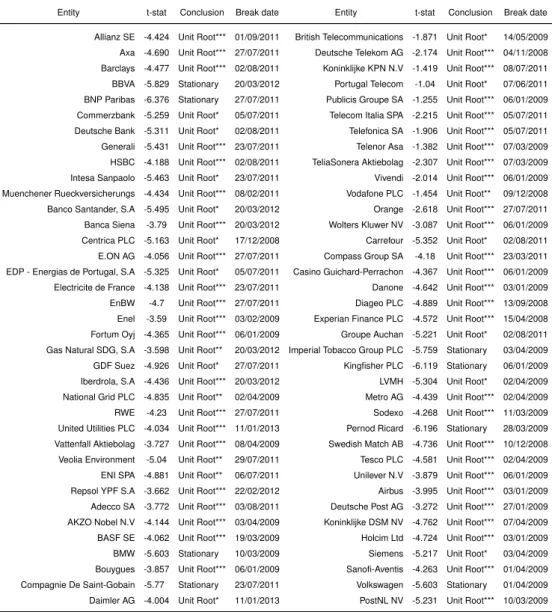
5.2
CDS-Bond Basis Structural Breaks
Table 10 reports the structural breaks detected in the time series
us-ing Bai and Perron (1998, 2003) method. A total number of 141 unknown
changes in the basis were detected for 69 firms.15. In 11 of those cases,
break dates can be explained by subprime crisis events, namely Bear
Sterns acquisition and Lehman Brothers collapse in March and
Septem-ber 2008 respectively. 20% of the structural changes occurred in 2009
when credit condition began to stabilize and reforms were implemented in
the CDS market. Financial support for Ireland, Greece and Portugal on
April, May 2010 and May 2011 respectively explain 45 out of 148
struc-tural breaks. In total the European Sovereign Debt crisis is responsible for
66% of the breaks. Besides, 14 breaks were detected around the period
in which Greece could not meet their obligations (March 2012).
5.3
Multivariate Regressions
Table 11 presents the CDS-Bond basis regression results for the
finan-cial firms. Results show that the proxy’s chosen better explain the
varia-tion in the CDS-Bond basis in the after break period. Besides, it is fair to
mention firm specific counterparty beta effect on the basis increases
sub-stantially also after the breaks.
Regarding CDS liquidity proxy, it proved significant only for 30% of the total
firms with a negative effect in the basis as expected. Bonds bid ask spread
have little significance in explaining basis dynamics particularly for the
fi-nancial sector. On the other hand, market option implied volatility proxy
VSTOXX, was highly significant in most of the cases and had an
aver-15for Deutsche Bank, Siena, Casino, Swedish and Unilever no structural change could
age positive effect of 100 basis points on the basis. Since higher volatility
is related to an increase of an entity default risk, this shows that CDS
spreads are more sensitive to VSTOXX changes than bond yield spreads.
The Euribor-EONIA spread proved significant in half of the sample with an
overall large effect on the CDS-Bond basis. In some cases, a one percent
increase in funding risk leads to an increase of nearly 4% in the basis.
Sur-prisingly, for some firms a negative sign was observed, possibly indicating
that for those, counterparty risk is significantly priced in the basis. Since
the sampling period comprises two financial turmoil events, there is the
risk that both markets were not pricing efficiently credit risk which could
bias the analysis. Market wide counterparty risk measured by the spread
between the primary dealers and ITraxx Europe index is statistically
rele-vant for 86% of the firms. While the risk of a counterparty default presents
a negative sign, its effect can be considered rather small since the
coeffi-cient is close to zero. On the other hand, when considering firm specific
counterparty betas, significance is found in 48 out of 74 companies with
mix results of impact in the basis. Only in 30% of the financial sector
re-sults were statistically significant, where a higher beta by one standard
deviation increases the CDS-Bond basis on average in 150 basis points.
The only exception was BNP Paribas which presented a decrease of 330
basis points.
6
Conclusion and Future Research
This study focused on assessing whether the no arbitrage condition
between CDS and bond markets held during the period covered. Apart
par-ity relation holds during normal times. Nevertheless, when markets suffer
from financial instability a negative impact arises around the basis.
Re-sults report that market conditions deteriorated more for non financial firms
during Lehman Brothers collapse while the reverse was observed in the
European sovereign debt crisis period. Counterparty risk effect on basis
dynamics after the break detected increased substantially, possibly
con-firming that before this type of risk was not correctly priced.
Cointegration tests performed on the basis suggest an increasing
per-centage of long run movement between CDS and bond spreads in the
firms included in the sample, when considering structural change in the
time series. Engle and Granger test documented cointegration in 55% of
the firms, contrasting with 50 out of 74 companies found in Gregory and
Hansen (1996) test.
Structural break detection revealed the existence of several changes in
the basis, where a total of 148 break dates were found falling particularly
on the 2011/2012 crisis but also on the subprime crisis period.
Further analysis of the basis could focus on assessing the lead-lag
re-lationship between CDS and Bond markets in the presence of a structural
break, through a rolling Granger Causality test. Both unit root and
coin-tegration testing across this study account for the possibility of only one
break in the time series. So, future research could extend the analysis
to multiple changes, such as the methodology presented in Westerlund
(2005). Besides, it could relate the implementation of a clearing
counter-party effects on the CDS-Bond basis and its implications relative to
7
References
Augustin, P. (2012). Squeezed Everywhere: Can We Learn Something New From the CDS-Bond Basis? Working Paper
Bai, J., and P. Collin-Dufresne, 2011, The determinants of the CDS-bond basis during the financial crisis of 2007–2009, Working paper, Columbia University.
Bai, J., and P. Perron (2003): `ıThe Computation and Analysis of Multiple Structural Change Models,Journal of Applied Econometrics, 18, 1022.
Blanco, R. S. Brennan, et al. (2005). ”An empirical analysis of the dynamic relationship between investment-grade bonds and credit default swaps.” The Journal of Finance 60(No.5):2255-2281
Collin-Dufresne, Pierre, Robert S. Goldstein, and J. Spencer Martin, 2001, “The determinants of credit spread changes”, Journal of Finance 56, 2177–2207
Coudert, Virginie and Matthieu Gex (2010) The Credit-Default Swap Market and the Settlement of Large De-faults, CEPII Working Paper 2010-17.
De Wit, J. (2006).”Exploring the CDS-Bond Basis” NBB Working Paper, No. 104, National Bank of Belgium Duffie, D. (1999).”Credit Swap Valuation” Financial Analysts Journal 55: 73-87
Engle,R.F and C. W. Granger (1987).”Co-integration and Error Correction: Representation, Estimation and Test-ing”. Econometrica 55(2): 251-276
Fontana, A.(2010).”The Persistent Negative CDS-Bond Basis during the 2007/08 Financial Crisis.” Ca’Foscari University of Venice, No13/WP/2007.
Garcia, R. and P. Perron (1996), An analysis of the real interest rate under regime switches, Review of Economics and Statistics 78, 111125
Gaspar, R.M and V. Fonseca (2011).”Counterparty and Liquidity Risk: an analysis of the negative basis”. ISEG, Technical University of Lisbon
Hansen, B.E. 2001. “The New Econometrics of Structural Change: Dating Changes in U.S. Labor Productivity,” Journal of Economic Perspectives, 15, 117-128.
Johansen, S., 1988, “Statistical Analysis of Cointegration Vectors,” Journal of Economic Dynamics and Control, Vol. 12, No. 2–3, pp. 231–254.
LongStaff, F. A., Mithal et al. (2005). ”Corporate Yield Spreads. Defaulr Risk or Liquidity? New Evidence from the Credit Default Swap Market.” The Journal of Finance 60(No.5):2213-2253
Nelson, CR. and C.I. Plosser, 1982, Trends versus random walks in macroeconomic time series: Some evi-dence and implications, Journal of Monetary Economics 10, 139-162.
Perron, P., 1989, The great crash, the oil price shock, and the unit root hypothesis, Econometrica 57, 1361-1401.
Perron, P. (2005) Dealing with Structural Breaks. In Palgrave Handbook of Econometrics (Patterson, K., and Mills, T.C., eds), 278-352
Pleus, J., and Westerfeld, S. The impact of counterparty risk on credit default swap pricing dynamics. The Journal of Credit Risk 8 (2012), 63–88.
Ericsson J., Jacobs, K., Oviedo, R., 2009. The Determinants of Credit Default Swap Premia.Journal of Financial and Quantitative Analysis 44, 109-132.
hypothesis. Journal of Business and Economic Statistics 10, 251-270.
Zhu, H.(2006). ”Determinants of Credit Spread Changes.” Journal of Financial Services Research 29(3): 211-235 Zhang, B.Y.-B., Zhou, H., Zhu, H., 2009. Explaining Credit Default Swap Spreads With the Equity Volatility and Jump Risks of Individual Firms. Review of Financial Studies 22, 5099-5131.
Table 3 Dataset Description
Financial Sector Ticker Country Rating Clearing Date Entity Ticker Country Rating Clearing Date Allianz SE ALV Germany A 10/05/2010 Commerzbank CBK Germany A
-Axa CS France A 10/05/2010 Deutsche Bank DB Germany A -Barclays BARC UK BBB - Generali ASSGEN Italy A 10/05/2010 Banca Monte Dei Paschi Di Siena S.P.A BMPS Italy - 10/05/2010 HSBC HSBA UK BBB
-Muenchener Rueckversicherungs MUV2 Germany BBB 03/05/2011 Intesa Sanpaolo ISP Italy AA 10/05/2010 Banco Santander, S.A SAN Spain AA 10/05/2010 BNP Paribas BNP France A
-BBVA BBVA Spain A 10/05/2010 Energy Sector
EDP - Energias de Portugal, S.A EDP Portugal BB 11/01/2010 EnBW EBK Germany A 11/01/2010 Electricite de France EDF France A 11/01/2010 Enel ENEL Italy BBB 14/12/2009 United Utilities PLC UU UK BBB 11/01/2010 E.ON AG EOAN Germany A 14/12/2009 Vattenfall Aktiebolag VATT Sweden NR 11/01/2010 Centrica PLC CNA UK A 14/12/2009 Veolia Environment VIE France BBB 11/01/2010 ENI SPA ENI Italy A 03/03/2014 Gas Natural SDG, S.A GAS Spain BBB 11/01/2010 Fortum Oyj FUM1V Finland A 11/01/2010 GDF Suez GSZ France A 11/01/2010 Repsol YPF S.A REP Spain BBB 08/03/2010 Iberdrola, S.A IBE Spain BBB 11/01/2010 RWE RWE Germany BBB 11/01/2010 National Grid PLC NG UK A 11/01/2010
Consumer
LVMH Moet Hennesy Louis Vitton MC France A 08/03/2010 Metro AG MEO Germany BBB 29/03/2010 Casino Guichard-Perrachon CO France BBB 29/03/2010 Pernod Ricard RI France BBB 03/03/2014 Compass Group SA CPG UK A 29/03/2010 Sodexo SW France A 29/03/2010 Imperial Tobacco Group PLC IMT UK BBB 11/04/2011 Airbus AIR France A
-Experian Finance PLC EXPN UK A 29/03/2010 Tesco PLC TSCO UK BBB 29/03/2010 Groupe Auchan AUCHAN France A 29/03/2010 Unilever N.V ULVR UK A 11/01/2010 Kingfisher PLC KGF UK BBB 11/04/2011 Carrefour CA France BBB 29/03/2010 Swedish Match AB SWMA Sweden BBB 11/04/2011 Diageo PLC DGE UK A 08/03/2010
Danone BN France A 08/03/2010 Auto&Industrials
Adecco SA ADEN Switzerland BBB 15/02/2010 Deutsche Post AG DPW Germany - 15/02/2010 AKZO Nobel N.V AKZO Netherlands BBB 19/04/2010 Koninklijke DSM NV DSM Netherlands A 19/04/2010 BASF SE BAS Germany A 19/04/2010 Holcim Ltd HOLN Switzerland BBB 15/02/2010 BMW BMW Germany A 08/03/2010 PostNL NV PNL Netherlands BBB 12/12/2011 Bouygues EN France BBB 11/04/2011 Siemens SIE Germany A 15/02/2010 Compagnie De Saint-Gobain SGO France BBB 15/02/2010 Sanofi-Aventis SAN France AA 10/05/2010 Daimler AG DAI Germany A 08/03/2010 Volkswagen VOW Germany A 08/03/2010 TMT
British Telecommunications BT/A UK BBB 01/02/2010 Telecom Italia SPA TIT Italia BB 01/02/2010 Deutsche Telekom AG DTE Germany BBB 01/02/2010 Telefonica SA TEF Spain BBB 01/02/2010 Koninklijke KPN N.V KPN Netherlands BBB 01/02/2010 Telenor Asa TEL Norway A 01/02/2010
Orange ORA France BBB 01/02/2010
Table 4 Primary Dealers List
Entity Barclays
Bank of America Merrill Lynch BNP Paribas
Citigroup Credit Suisse Deutsche Bank Goldman Sachs HSBC
JPMorgan Morgan Stanley Nomura UBS
Table 5 ZA Test: CDS Levels
Table 6 ZA test: ∆(CDS)
Table 7 ZA Test: Bond spreads
Table 8 ZA test: ∆(Bondspread)
Table 9 Cointegration Results with Structural Break
Table 10 Bai and Perron (2003) Detected Structural Breaks
Entity Break Dates Entity Break Dates Allianz SE 30/04/2012 Deutsche Telekom AG 15/10/2010 17/04/2009
Generali 02/03/2012 18/09/2008 14/01/2010 Portugal Telecom 09/03/2012 17/04/2008 26/05/2009 Banco Santander, S.A 17/01/2013 Orange 31/08/2011 04/08/2010
Axa 19/03/2010 07/07/2011 Publicis Groupe SA 15/05/2012 18/01/2011
Barclays 19/04/2010 29/07/2011 17/12/2012 21/04/2010 Telecom Italia SPA 02/06/2010 15/05/2009 26/07/2010 BNP Paribas 30/10/2012 16/06/2008 12/11/2010 Telefonica SA 12/06/2009 04/02/2013
BBVA 01/02/2013 Telenor Asa 22/07/2009 30/10/2012
Commerzbank 02/09/2010 11/03/2009 TeliaSonera Aktiebolag 04/08/2009 07/05/2012 22/02/2013 Deutsche Bank No Break Vodafone PLC 11/01/2010 12/10/2011
HSBC 27/07/2010 09/08/2012 Vivendi 08/07/2009 17/10/2011
Intesa Sanpaolo 27/02/2012 17/06/2008 British Telecommunications 06/07/2012 07/02/2012 17/12/2010 10/11/2010 Banca Siena S.P.A No Break Koninklijke KPN N.V 03/04/2012
Muenchener 16/09/2008 Wolters Kluwer NV 11/01/2010
Centrica PLC 13/08/2010 Airbus 08/09/2011 11/12/2012 E.ON AG 24/08/2011 13/05/2009 09/08/2010 Casino Guichard No Break Electricite de France 28/07/2011 01/02/2010 13/01/2009 Danone 30/09/2009 25/02/2013
Enel 26/11/2008 Diageo PLC 26/11/2009 12/10/2011 Fortum Oyj 28/06/2010 12/07/2011 30/09/2010 Imperial Tobacco PLC 04/04/2012
Iberdrola, S.A 16/04/2009 05/10/2010 25/02/2013 LVMH 29/09/2011 22/02/2013 Gas Natural SDG, S.A 08/07/2009 20/03/2012 Pernod Ricard 27/05/2009 24/01/2012
GDF Suez 08/06/2009 12/04/2011 Sodexo 24/02/2012
National Grid PLC 02/12/2008 Swedish Match AB No Break
Repsol YPF S.A 08/12/2011 21/10/2008 Tesco PLC 08/06/2009 31/10/2011 28/10/2011 06/12/2012 United Utilities PLC 21/01/2010 18/09/2012 Carrefour 21/06/2011 13/08/2009
Vattenfall Aktiebolag 30/09/2009 28/10/2011 Compass Group SA 01/09/2009 10/02/2012 07/09/2012 ENI SPA 03/04/2012 Experian Finance PLC 03/02/2010 09/05/2008
EnBW 17/08/2009 05/01/2010 Groupe Auchan 29/09/2009 31/10/2011 RWE 15/07/2010 19/02/2013 22/02/2013 Kingfisher PLC 10/08/2009 29/07/2011 Veolia Environment 11/04/2011 15/06/2009 Metro AG 21/09/2011 29/07/2011
EDP, S.A 12/10/2011 04/08/2009 Unilever N.V No Break Adecco SA 14/05/2012 Koninklijke DSM NV 08/08/2012 16/03/2009 08/08/2012 AKZO Nobel N.V 05/03/2012 28/07/2008 04/04/2012 21/03/2011 Holcim Ltd 05/05/2009 02/09/2011 11/12/2012
BASF SE 01/09/2011 Siemens 09/04/2008 Bouygues 13/04/2012 16/02/2009 19/08/2010 Sanofi-Aventis 17/10/2011 Compagnie De Saint-Gobain 17/04/2012 19/08/2010 Volkswagen 18/03/2011
Table 11 Time Series Determinants of CDS-Bond Basis: Multivariate Regressions - Financial Sector
Firm Basˆcds Bas ˆbond ccp agg Betai VSTOXX EUEO Adj R2 Deutsche Bank No Break 0.02144 18.7538*** -0.0825 361,71*** 0.9288*** 3547.279*** 0.09
Allianz Before -0.2092* -3.6236 0.1407*** 56.3534 -0.5534*** -2332.855*** 0.0793 After 0.24*** -0.14 0.5181*** 2555.41*** -0.4*** -865.44 0.2054 Santander Before 0.074 -0.24 0.019 62.43 0.91 -1085.25 0.02
After 0.28** 1.62 -1.74*** -2645.23 1.56*** 3581.499 0.41 BBVA Before 0.01 0.4 -0.46*** 32.66 0.66*** 3727.025** 0.07 After 0.24** 4.5 -1.55*** 0 1.13*** -11.48 0.41 HSBC Before 0.3 0.06 -0.14 99.74*** 0.42*** 2305.39** 0.04 After 0.32 5.61 -0.31*** -427.07*** 1.22 -1144.59 0.09 Intesa Before 0.05 -0.45 -0.12*** -23.9 0.62** 1902.27 0.09 After 0.11 -0.67 -1.36*** -1199.19 1.84*** -11015.03*** 0.2 Siena No Break
Muenchener Before 0 -36.37 -0.48*** 17.1 -0.48 2027.39 0.31 After 0.12 19.94** -0.17*** -58.87 0.28** 127.69 0.33 AXA Before -0.66* 17.93 0.28** -13.34 -0.26 -3254.184 0.07 After 0.3848* 1.48 0.3365 -429.86 0.5767 -950.01 0.26 Barclays Before -0.19 19.25 0.19* 52.55 -0.15 -996.82 0.62 After 0.14 -0.32 0.32** -1409.34 0.33 124.17 0.76 Generali Before 0.0432 -8.1*** -0.82*** 17.03*** 2.08*** 1902.65*** 0.2877
After -0.32** -0.08 -0.32*** -0.31 0.83*** 3231.59** 0.1392 Commerzbank Before 0.3 0.06 -0.69** 99.74** 0.42*** 2305.97*** 0.04
After 0.32*** 5.61** -0.31 -427.07*** 1.22*** -1144.59 0.09 BNP Before 0.26 1.06 -0.35*** -126.25* 0.57*** -1203.97 0.03 After -1.18 12.19 -2.57*** -5201.37 -0.02 -204.13 0.05
Table 12 Time Series Determinants of CDS-Bond Basis: Multivariate Regressions - Non Financial
Firm Basˆcds Bas ˆbond ccp agg Betai VSTOXX EUEO Adj R2 Before -0.14 -31.13*** -0.07 -0.92 0.92*** 1412.48 0.07 Adecco After 0.16*** -32.12 -0.13 -825.64*** 0.84*** 4162.95 0.25 Before 0.22 14.16 -0.42*** -98.06* 0.13 2865.975 0.04 Akzo After 0.09 -6.93 -0.16*** -381.22 0.61*** 627.65 0.09 Before 0.07 -3.26 -0.12*** -7.83 0.54*** 1295.65** 0.09 Basf After 0.09 -1.13 -0.08** -131.02 0.75*** 1793.81** 0.16 Before 0.03 0.5 -0.11*** -58.79*** 0.53*** 1344.30** 0.09 Bouygues After 0.20*** -0.96 -0.44*** -1669.37*** 0.87*** 1027.32 0.20 Before 0.12 8.16 -0.26*** -11.04 0.92*** 3832.15*** 0.12 Cie After 0.10* -0.21 -0.45*** -5602.25*** 0.95*** 918.02 0.25 Before 0.32** 7.86 -0.19*** -45.83 1.09*** -300.38 0.10 Daimler After 0.12 -9.54 -0.28*** -381.08 1.00*** 462.17 0.21 Before 0.05 -22.69** -0.19*** -64.58*** 1.08*** -1070.241 0.08 Deutsche Post After 0.19 12.86 -0.3*** 9.02 1.07*** 593.63 0.18 Before -0.01 -0.93 -0.08** 13.60 0.42*** 856.41 0.03 DSM After 0.37** 5.02 750.32 0.22** 2307.4 0.1
Before 0.5*** -43.42 0.12 -346.67*** 1.71*** -1297.63 0.26 Holcim After 0.34*** 7.36 -0.22*** -1854.73** 0.55*** 1183.58 0.25 Before 0.49 3184.71 -0.71*** -20.95 1.12*** 2588.12 0.39 Siemens After -0.09 -5.18 -0.28*** -35.30 1.26*** 3342.25*** 0.17 Before 0.13 -2.46 -0.03 34.60* 0.41*** 635.19 0.06 Sanofi After 0.09 3.19 -0.17*** -160.95 0.51*** -118.94 0.16 Before 0.01 0.01* -0.31*** -40.50 0.97*** 605.45 0.11 VW After 0.04 -4.68 -0.3*** -143.51 0.89*** 505.30 0.17 Before 0.04 -11.72 -0.00 -35.30 0.76** -4921.23** 0.04 BMW After -0.01 -16.87*** -0.29*** -221.477 0.80*** 954.51 0.22 Before -0.17*** -8.81** -0.5** -83.40*** 0.50*** 306.88 0.14 PostNL After 0.23*** -0.86 -0.4*** 153.13** 0.88*** 425.83 0.17