Regional input-output tables and models

Faculdade de Economia

Universidade de Coimbra

Regional input-output tables and models

Interregional trade estimation and input-output modelling

based on total use rectangular tables

Ana Lúcia Marto Sargento

Dissertação para Doutoramento em Economia, na especialidade de

Planeamento e Economia Regional, apresentada na Faculdade de

Economia da Universidade de Coimbra, orientada por: Professor Pedro

INDEX

ABSTRACT ... 9

RESUMO ... 11

INTRODUCTION... 13

CHAPTER 1 – INTRODUCING INPUT-OUTPUT ANALYSIS AT THE

REGIONAL LEVEL: BASIC NOTIONS AND SPECIFIC ISSUES... 19

1.1. INTRODUCTION... 20

1.2. FOUNDATIONS OF INPUT-OUTPUT: BASIC INPUT-OUTPUT TABLE AND DEDUCTION OF THE LEONTIEF MODEL. ... 27

1.3. REGIONAL INPUT-OUTPUT MODELS. ... 36

1.3.1 Single-region model... 38

1.3.2 Leontief’s intranational model... 42

1.3.3 Isard’s IRIO (interregional input-output model)... 47

1.3.4 Chenery-Moses’s MRIO (multiregional input-output model)... 53

1.3.5 Riefler-Tiebout’s bi-regional input-output model. ... 59

1.3.6 Trade coefficient stability. ... 62

1.4. OBTAINING THE DATA FOR REGIONAL INPUT-OUTPUT MODELS: TABLE CONSTRUCTION... 63

1.4.1 Survey table ... 64

1.4.2 Non-survey and hybrid techniques. ... 65

1.4.3 Matrix adjustment methods: the particular case of RAS. ... 70

1.4.4 Evaluating the accuracy of estimated input-output tables. ... 77

1.5. THE SPECIFIC FEATURES OF THE NATIONAL TABLES AND THEIR IMPLICATIONS ON THE REGIONAL TABLE CONSTRUCTION PROCESSES BY HYBRID OR NON-SURVEY METHODS. ... 85

1.5.1 “Commodity-by-industry” accounts. ... 86

1.5.2 Regionalizing a national Make and Use table... 92

1.5.4 Techniques used to estimate intra-regional use flows from total use flows. 97

1.6. MODELS TO ASSESS INTERREGIONAL TRADE DATA... 109

1.6.1 The relevance and nature of external trade in regional economies... 109

1.6.2 Determining net exports in single-region input-output models. ... 112

1.6.3 From net to gross trade flows: the problem of crosshauling... 121

1.7. CONCLUSIONS... 126

1.8. NOTATION... 130

1.9. REFERENCES... 134

CHAPTER 2 – DETERMINING INTERREGIONAL TRADE FLOWS

IN A MANY-REGION SYSTEM... 145

2.1 INTRODUCTION. ... 146

2.2 INTERREGIONAL TRADE FLOW ESTIMATION AS A SPATIAL INTERACTION PROBLEM... 149

2.3 THEORETICAL REVIEW OF THE SPATIAL INTERACTION MODELS PROPOSED TO ESTIMATE TRADE FLOWS... 153

2.3.1 Gravity models. ... 153

2.3.2 Entropy-based models... 160

2.3.3 Information theory models... 171

2.3.4 Behaviour models... 179

2.4 EMPIRICAL EXAMINATION OF THE GRAVITY MODEL IN TWO DIFFERENT INFORMATION CONTEXTS: EXPLANATION AND ESTIMATION. ... 184

2.4.1 Type (a) information context... 184

2.4.1.1 Gravity model extensions to trade applications in type (a) information context. 185 2.4.1.1.1 Augmenting the gravity equation with additional explanatory variables. 185 2.4.1.1.2 Formal specification of spatial dependence... 186

2.4.1.3.1 Basic gravity equation... 198

2.4.1.3.2 Spatial econometric application. ... 201

2.4.2 Type (b) information context... 214

2.5 ABSOLUTE AND ANALYTICAL COMPARISON BETWEEN DIFFERENT INTERREGIONAL TRADE ESTIMATION METHODS. ... 219

2.5.1 Multi-regional input-output system assemblage... 220

2.5.2 Development of the multi-regional input-output model... 229

2.5.3 Alternative methodologies to estimate interregional trade. ... 232

2.5.4 Comparison between the results provided by the different estimation methods. 238 2.5.5 Input-output model sensitivity to the alternative methodologies of interregional trade estimation. ... 241

2.6 CONCLUSIONS... 252

2.7 REFERENCES... 255

CHAPTER 3 – INPUT-OUTPUT MODELLING BASED ON TOTAL

USE RECTANGULAR TABLES. ... 264

3.1 INTRODUCTION. ... 265

3.2 THE THREE FUNDAMENTAL CRITERIA FOR THE CONSTRUCTION OF INPUT -OUTPUT TABLES: DEFINITIONS AND IMPLICATIONS... 271

3.2.1 Symmetric and rectangular input-output tables revisited... 274

3.2.2 Total use flows versus domestic use flows. ... 276

3.2.3 Basic versus purchasers’ prices... 276

3.3 INPUT-OUTPUT TABLES IN THE PORTUGUESE NATIONAL ACCOUNTS. ... 279

3.4 INPUT-OUTPUT MODELLING BASED ON THE TOTAL USE M&U MATRIX, AT PURCHASERS’ PRICES. ... 280

3.4.1 The proposed hypothesis to deal with intermediate and final use of imported products... 281

3.4.2 The proposed hypothesis to deal with margins and taxes less subsidies on products... 284

3.4.3 Two alternative hypotheses to connect the products’ output with the industries’ output on the rectangular table: Industry technology assumption (ITA) and

Commodity technology assumption (CTA). ... 287

3.4.3.1 Model development under each of the hypotheses. ... 291

3.4.3.2 Partitioned matrix inverse: calculation and analysis... 297

3.4.3.3 The present and past literature debate on ITA versus CTA... 302

3.5 PRACTICAL APPLICATION. ... 310

3.5.1 Calculation of different multipliers on the basis of the rectangular model, using the Portuguese M&U table. ... 310

3.5.2 Obtaining the symmetric input-output table (SIOT) from the rectangular one. 313 3.5.2.1 Product-by-product symmetric tables. ... 314

3.5.2.2 Industry-by-industry symmetric tables. ... 319

3.5.3 Computation of the symmetric input-output table’s Leontief inverse and the correspondent multipliers. ... 320

3.5.4 Direct requirements matrices in the rectangular and in the symmetric model. 323 3.6 CONCLUSIONS... 326 3.7 NOTATION... 329 3.8 REFERENCES... 331

CONCLUSIONS... 336

ACKNOWLEDGEMENTS... 344

ABSTRACT

The present research concerns the study of input-output modelling and input-output table construction, when applied at the regional level. Input-output models, at the national or regional level, are known as a fundamental tool for economic analysis. Yet, in order to apply such models, the researcher must have access to the correspondent input-output tables. National-level tables are currently published by the national statistical offices according to well-defined conventions. The same, however, cannot be said about regional tables which are not provided as a rule by official statistics organisms. Being so, a great part of input-output research is still dedicated to the study of techniques for input-output table gathering.

This dissertation is, in such context, divided into three chapters. The first one is mainly theoretical, aiming to review the basic principles underlying input-output analysis at the regional level. The second and third chapters constitute the research’s practical contribution, focused on two major issues, respectively: 1) interregional trade estimation and 2) input-output modelling on the basis of total-use rectangular table at purchasers’ prices.

In most countries, survey-based interregional trade data does not exist. However, even when some simplifying assumptions are used in the model, a minimum amount of data on interregional trade is always necessary, in order for the model to succeed in capturing spillover and feedback effects caused by the interregional linkages. In order to evaluate the reasonability of using indirect interregional trade flows estimates, a comparison was made between alternative methodologies (with special focus on gravitational models), assessing the sensitivity of the model results. Such comparison allowed to conclude that the results of the input-output model are not greatly affected by the insertion of different

trade flow values. Thus, the results obtained do not reject the reasonability of using indirect estimates for interregional trade, whenever survey-based data is unavailable.

The official input-output tables are published on a total-use rectangular format, which is different from the lay-out upon which traditional input-output models were developed (domestic use symmetric tables). The objective here was to demonstrate the equivalence in the results of the input-output model between two alternative procedures: 1) to convert the available input-output table into a domestic-flow symmetric table at basic prices and then implement the input-output model; 2) to perform the direct modelling of the original table (the total-flow rectangular table at purchasers’ prices). It has been concluded that, when the same set of hypotheses is used, there is no advantage in making a previous transformation of the original tables into the symmetric format and a previous calculation of domestic flows, since the results of the model are exactly the same.

RESUMO

O presente trabalho de investigação incide sobre modelos de input-output, a nível regional. Os modelos de input-output, ao nível nacional ou regional, são reconhecidos como uma ferramenta fundamental de análise económica. Contudo, para que tais modelos sejam aplicáveis, é necessário dispor dos quadros de input-output correspondentes. Actualmente, os quadros nacionais de input-output são publicados de forma regular pelos organismos de estatística oficiais de cada país, de acordo com convenções internacionais bem definidas. O mesmo não pode ser afirmado sobre os quadros regionais, que não fazem parte das publicações estatísticas oficiais. Sendo assim, uma boa parte da investigação na área do input-output recai ainda sobre as técnicas para a construção de quadros a nível regional.

Neste contexto, a presente dissertação divide-se em três capítulos. O primeiro possui uma natureza substancialmente teórica, pretendendo fazer uma revisão dos princípios básicos subjacentes à análise input-output ao nível regional. O segundo e terceiro capítulos constituem o contributo prático da investigação, focando dois temas específicos: 1) estimação do comércio inter-regional e 2) modelização input-output baseada em quadros rectangulares de uso total, a preços de aquisição.

Na maioria dos países não existem dados directos sobre o comércio inter-regional. No entanto, há um mínimo de informação sobre estes fluxos que é imprescindível, mesmo que no modelo sejam usadas algumas hipóteses simplificadoras. Sem essa informação, o modelo é incapaz de captar os efeitos de spillover (extravazamento) e de feedback (realimentação) causados pelas ligações inter-regionais. Com o intuito de avaliar a razoabilidade de usar estimativas indirectas para os fluxos de comércio inter-regional, foi feita uma comparação entre metodologias alternativas (com especial enfoque nos modelos gravitacionais), medindo a sensibilidade dos resultados do modelo. Esta

comparação permitiu-nos concluir que os resultados do modelo input-output não são afectados em grande medida pela inserção de diferentes valores de fluxos de comércio. Assim, os resultados obtidos não rejeitam a razoabilidade de usar estimativas indirectas para o comércio inter-regional, sempre que não estejam disponíveis dados recolhidos directamente.

Os quadros oficiais de input-output são publicados num formato rectangular, com fluxos de uso total, sendo por isso diferentes do molde tradicional sobre o qual foram desenvolvidos os modelos de input-output tradicionais (quadros simétricos com fluxos de uso doméstico). O objectivo aqui era o de demonstrar a equivalência nos resultados do modelo de input-output quando são aplicados dois procedimentos alternativos: 1) converter o quadro input-output publicado para um quadro simétrico de fluxos domésticos a preços de base e só depois implementar o modelo de input-output; 2) desenvolver o modelo directamente a partir do quadro original (o quadro rectangular de fluxos totais a preços de aquisição). Concluiu-se que, quando se utiliza o mesmo conjunto de hipóteses, não há qualquer vantagem em proceder a uma transformação prévia dos quadros originais para o formato simétrico a fluxos domésticos, dado que os resultados do modelo são exactamente os mesmos.

The input-output framework relies upon a very simple, yet essential notion, according to which the output is obtained through the consumption of production factors (inputs) which can be, in their turn, the output of other industries. The fundamental recognition of the underlying system of interactions and interdependencies between industries is at the core of the input-output tables and model construction.

This work is concerned with the study of the input-output analysis, when applied at the sub-national or regional level. Regional input-output analysis involves, on the one hand, the access to a very detailed statistical tool about the economy we are focusing on: the regional input-output table. These tables represent a comprehensive portrait of the region describing, among other things: the technology implicit in the production process, the dependencies between industries, the regional consumption patterns and the inter-dependencies between the region and the rest of the world. They may constitute an important instrument in the production of regional accounts, namely to balance the income, expenditure and production estimates of regional GDP. The information comprised in regional input-output tables permits also the conduction of interesting studies about the regional economic structure, such as the identification of key sectors or crucial interregional linkages. Yet, the most widespread use of the regional input-output tables consists in the input-output models, allowing for the assessment of economic impacts resulting from exogenous changes in final demand, which may be caused by different regional policies, for instance: regional development policies or investment on transportation infrastructures. Such sort of regional analysis is receiving increasing interest by the research community, as a results of the growing economic integration (especially in the European Union), with the associated efforts in reducing regional disparities within each country and between members. This should imply the need for some reliable accounting system that helps the identification of regional impacts and interregional spillover effects and which may be used as an instrument to monitor regional policies.

the researcher intends to link several regions through a multiregional input-output system. Regional input-output tables are not provided as a rule by official statistics organisms. In the majority of the European countries, only some regional indicators are published on a regular basis, such as: regional output by industry, regional value added by industry and total intermediate consumption by industry. These data may be taken as a starting point to assemble the individual regional tables, using a combination of non-survey and survey methods and taking the national input-output table as a reference to obtain the regional counterpart. It is consensual that the more direct information is incorporated in the table, the more accurately it tends to reflect regional reality. However, the introduction of direct information implies higher costs, which forces the researcher to make this in a selective way (more or less restrictively, depending on the resources available to conduct regional surveys). The attempt of assembling regional output tables and multiregional input-output systems using limited direct information is often considered to be an unfeasible endeavor. We do not agree with this view. Conversely, we share the perceptible opinion of other researchers which have devoted their efforts to the construction of regional input-output models, even in developing countries, in which information is more limited. Yet, in order to obtain the best possible results, we consider that it is necessary to:

• Find an adequate equilibrium in the existing trade-off between model complexity and model construction practicability. This means that the existing models must be evaluated in face of the information availability in each particular case.

• Study and evaluate different non-survey methodologies to estimate inexistent information (such as interregional trade) and critically analyze the implicit hypotheses, testing the sensitivity of the model solutions to the techniques and hypotheses assumed.

• Get the maximum benefit of the existing information and try to adapt the proposed models in order to fit into the (sometimes more advantageous) format in which information is provided. For example, traditional input-output models were developed within the symmetric framework, meaning that the supporting input-output tables were product-by-product or industry-by-industry tables. Currently, however, most of the countries compile and publish their national input-output

tables in the rectangular or Make and Use format (introduced by the United Nations in 1960’s), requiring some adaptation in the existing models.

With the present work we aim to achieve the following broad objectives, which correspond to the three Chapters included in this dissertation:

• To make a broad review of the state of knowledge regarding input-output modeling and input-output table construction at the regional level, paying special attention to the quantitative and qualitative disagreement between the data requirements implicit in the traditional input-output models and the usually available data. We intend to accomplish this objective in Chapter 1 of the Dissertation: “Introducing Input-output analysis at the regional level: basic notions and specific issues”.

• To study and test methodologies to overcome the above mentioned mismatch between data requirements and data availability, focusing on two specific issues:

o Interregional trade indirect estimation, as a viable alternative to solve the common difficulty in regional table construction – the inexistence of survey-based interregional trade data. This will be the focus of Chapter 2: “Determining interregional trade flows in a many-region system”.

o Input-output modeling based on total use rectangular input-output tables, implying the adaptation of the traditional input-output model to the format in which the input-output database (published on a regular basis for the national level) is currently provided. This issue is considered in Chapter 3: “Input-output modeling based on total use rectangular tables”.

The research is guided towards the answer to the following questions (of which some involve specific concepts to be explained in the development of the dissertation):

• What is the state of the art of regional input-output table construction and modelling?

• How easy is it to apply the existing models to countries like Portugal, with limited regional and interregional information?

• What models have been used to indirectly estimate interregional trade flows? • What is their actual applicability under a context of very limited a priori

information?

• When applying different interregional trade estimation methodologies:

o What is the degree of closeness of each estimated matrix to the real matrix of flows?

o Which method generates the most accurate estimated matrix?

o How sensitive are the values obtained in the final trade matrix to different estimating methods?

o How sensitive is the solution of the input-output model to the insertion of different interregional trade values? In other words, how important is the choice of interregional trade estimation method to the solution of the input-output model?

• What procedures and related hypotheses may be used to perform input-output modelling when the basic data consists of a total-use rectangular table at purchasers’ prices, with no available import matrix?

• Is it advantageous to perform a previous transformation of the original tables into the symmetric format and a previous calculation of domestic flows, before implementing the model?

The main motivation to the conduction of this research is a very practical one: to help the researchers in defining their strategy in future efforts of multiregional input-output table construction and modelling. We hope to give our contribution to the construction of such model to the Portuguese economy. Despite being heavily theoretical, the underneath intention of this work is evident in various parts of the dissertation.

CHAPTER 1 – INTRODUCING INPUT-OUTPUT

ANALYSIS AT THE REGIONAL LEVEL: BASIC

1.1.

Introduction

The main objective of the well known input-output model, developed by Leontief in the late 1930s, is to study the interdependence among the different sectors in any economy (Miller and Blair, 1985). This tool holds upon a very simple, yet essential notion, according to which the output is obtained through the consumption of production factors (inputs) which can be, in their turn, the output of other industries. Hence, one of the principal tasks of input-output analysis is to identify the indirect demands concerning the intermediate consumptions necessary to generate the outputs.

The origins of the basic notion behind the input-output model go back to the 18th century, when Quesnay published the “Tableau Economique”. His objective was to describe the economic transactions established between three social classes: landowners, farmers and rural workers (productive class) and the sterile class, composed by artisans and merchants (this classification reflects the physiocrats’ philosophy, according to which agriculture was the only wealth generating sector).

Over more than one century, this idea of economic interdependence had a new and important contribution, with the work developed by Walras1. This economist introduced the general equilibrium model, aiming to determine prices and quantities of all economic markets. In this model Walras used a set of production coefficients very similar to the ones defined a posteriori in the Leontief’s input-output model: they compared the amount of production factors used in production with the total output obtained (Miller and Blair, 1985).

The perception and depiction of the interactions among the different economic activities (besides the spatial dimension which is being considered) allows, on the one hand, the access to a very detailed statistical tool about the economy we are focusing on: the

output table. An input-output table records the “flows of products from each industrial sector considered as a producer to each of the sectors considered as consumers” (Miller and Blair, 1985, p. 2). This table gives us a quite complete picture of the economy at some specific point in time, providing estimates for an important set of macroeconomic aggregates (production, demand components, value added and trade flows) and disaggregating these among the different industries and products. Besides, the input-output table is a suitable instrument to perform structural analysis of the correspondent economy, depicting the interdependence between its different sectors and between the economy and the rest of the world (ISEG/CIRU, 2004). On the other hand, the input-output table provides an important database to the construction of input-input-output models which may be used, for example, to evaluate the economic impact caused by exogenous changes in final demand (Miller, 1998).

The original applications of the input-output model were made at a nation-wide level2. However, the interest in extending the application of the same framework to spatial units different from the country (usually, sub-national regions) led to some modifications in the national model, originating a set of regional input-output models. According to Miller and Blair (1985), there are two specific characteristics referring to the regional dimension which make evident and necessary the distinction between national and regional input-output models. First, the productive structure of each region is specific, probably being very different from the national one; second, the smaller the focusing economy, the more it depends on the exterior world (this including the other regions of the same country and other countries), making exports and imports to become more important in determining the region’s demand and supply.

Since the 1950’s, different regional input-output models were developed, being distinguished through the following criteria: (1) the number of regions taken into account; (2) the recognition (or not) of interregional linkages; (3) the degree of detail implicit in interregional trade flows (which is related to the degree of detail demanded for the

2

An example of this is the pioneering application of Leontief to the United States that became public through the book “The Structure of the American Economy, 1919-1929”, published for the first time in 1941.

output data) and (4) the kind of hypotheses assumed to estimate trade coefficients. The first criterion is used to distinguish the single-region model from the several types of models designed to systems with more than one region. The single-region model seeks to capture intra-regional effects alone. So, its crucial limitation consists of the fact that it ignores the effects caused by the linkages between this region and the others. But in reality, when one region increases its production, as a reaction to some exogenous change in its final demand for example, some of the inputs needed to answer the production augment will come from the remaining regions, originating an increase of production in these regions – these are the spillover effects. The remaining regions, in turn, may need to import inputs from other regions (probably including the first region) to use in their own production. These involve the concept of interregional feedback effects: those which are caused by the first region in itself, through the interactions it performs with the remaining regions (Miller, 1998). The seminal applications of input-output analysis to systems with more that one region, capturing the effects caused by the interconnections between the different regions (which corresponds to the second criterion previously referred), had the fundamental contributions of Walter Isard (Glasmeier, 2004). These contributions originated the interregional model also known as Isard’s model. Practical difficulties in implementing the interregional model, mainly due to its high requirements in terms of interregional trade data, motivated the emergence of multi-regional models (of which the Chenery-Moses model is the most popular). As we shall see latter on this Chapter, the different many-region models are distinguishable through the third and fourth criteria mentioned above.

This brief introduction to regional input-output models makes clear that their implementation requires the access to some data on interregional trade flows (more or less detailed, depending on the specific type of regional input-output model). But how relevant are actually interregional trade flows to regional economies? Some regional studies have proved that trade flows established between one region and the remaining regions tend to be more significant than trade flows established between the same region and foreign countries (Munroe and Hewings, 1999). Moreover, interregional trade is

One of the reasons for the rapid growth of interregional trade is the fact that it is currently replacing much of the intra-regional transactions, in a process called “hollowing-out”: it implies that the density of relations within the regional economy tends to diminish, in favour of interregional linkages (Polenske and Hewings, 2004). Given its relative importance in the region’s external trade, the knowledge of the volume and nature of interregional trade flows constitutes a critical issue for regional analysis. For example, a deficit in the region’s trade balance means that the region relies on income transfer and/or granting of savings from other regions, within the country or from the rest of the world (Ramos and Sargento, 2003). In a more detailed perspective, knowledge about regional external trade, segmented by commodities, allows us to characterize productive specialization, foresee eventual productive weaknesses as well as determine the region’s dependency on the exterior (or in some cases the exterior’s dependency on the region) regarding to the supply of different commodities. In spite of its recognized importance, interregional trade flows established between regions of the same country constitute precisely the hardest data to find among the set of data necessary to implement the input-output model.

The previous paragraph leads us to the first of the fundamental issues underlying the present work, which also constitutes one of the main challenges of regional input-output researchers: obtaining the regional data necessary to implement input-output models, with special concern in interregional trade. The existing regional data, provided by the official organisms of statistics, is usually “less than perfect”, meaning that it is more or less distant from the ideal set of data required by each type of regional input-output model. Facing this problem, the researcher may follow two alternatives (or do both): adapt the model to the existing data and / or estimate (or directly collect) the inexistent data. Even when some adaptation is made, through the use of some assumptions, a minimum amount of data on interregional trade (besides other input-output table components) is always necessary, so that the model succeeds in capturing spillover and feedback effects caused by the interregional linkages. Being so, some techniques must be adopted to assess those data. These techniques can be classified according to the degree of incorporation of direct regional information. Most of the researchers use hybrid

methods, combining some survey information with non-survey techniques, in which specific regional indicators are applied to convert national values into regional ones. It is consensual that the more direct information is incorporated in the table, the more accurately it tends to reflect regional reality. However, the introduction of direct information implies higher costs, which forces the researcher to make this in a selective way (more or less restrictively, depending on the resources available to conduct regional surveys). Besides, even if the research team doesn’t face any restrictions in terms of money, time, manpower or logistic resources, this doesn’t guarantee that a pure survey-based table is completely exempt of errors. In fact, according to Jensen (1980), errors in survey tables can result from errors in the process of gathering the data (for example: errors arising from incorrect definition of the sample, hiding of information or lack of concern in answering the questionnaires by the respondents) or errors in compilation procedures. Besides, other problems may arise whenever the questions included in the questionnaires require very detailed information to which some respondents may not be able to answer. In this context, Jensen (1980) argues that the concept of holistic accuracy must be privileged, meaning that the assembly of direct information should be directed only towards the larger or most important elements of the economy being studied, thus ensuring a correct representation of the structure of the economy, in general terms (Hewings, 1983). In other words, hybrid methods assure the best compromise between accuracy and required resources. The theoretical review of the main techniques used to generate undisclosed data will be made on this Chapter. In what concerns specifically to the problem interregional trade estimation, the main existing techniques will be discussed on Chapter 2.

An additional important challenge faced by input-output researchers consists in adapting the traditional input-output models in order to fit them into the specific format in which information is available. The fact is that, sometimes, input-output rough data exists, but it is provided in a different way from that underlying the traditional input-output models. For example, traditional input-output models were developed within the symmetric framework, meaning that the supporting input-output tables were product-by-product or

both rows and columns, showing the amounts of each product used in the production of which other products. In turn, industry-by-industry tables have industries as the dimension of both rows and columns, showing the amounts of output of each industry used in the production of which other industries (UN, 1993). Currently, however, most of the countries compile and publish their national input-output tables in the rectangular or Make and Use format (introduced by the United Nations in 1960’s). In this framework, two dimensions are simultaneously considered (industries and products) and two tables are essential: the Use table, which describes the consumption of products j by the several industries i, and the Make table that represents the distribution of the industries’ output by the several products. In conjunction, these tables depict how supplies of different products originate from domestic industries and imports and how those products are used by the different intermediate or final users, including exports (UN, 1993). The procedures and hypotheses adopted in input-output table construction as well as in input-output modelling should be suited to fit this data format.

Another example of non-coincidence between the model’s data requirements and data availability is at the intermediate transactions table: the nuclear part of an input-output table, which represents the intermediate consumption of the several products made by the different industries. In some countries, like Portugal, the national intermediate transactions table is provided in a total use basis, meaning that the amount of products recorded as inputs in the intermediate consumption of the different industries comprise either nationally produced or imported products. However, some input-output models involve the determination of impacts within the region (or within the nation, depending on the spatial dimension being considered), implying that the computed effects should be cleaned from effects on imports. In such case, the model should be adapted, under some hypotheses, to fit the available total use data.

The choice of the proper hypotheses to develop national and regional input-output models when input-output data is not available in the traditional format is the second fundamental issue underlying the present work. Being so, we aim to provide in this Chapter some fundamental concepts on the accounting systems in which input-output

data are currently provided, so that latter on this work (in Chapter 3) the above referred hypotheses can be discussed in a clearer way. Obviously, instead of adapting the models to fit the existing data, an alternative consists in transforming the data in order to match the hypotheses beneath the traditional models. In the above mentioned situations this would imply: (1) converting the Make and Use format into a symmetric format previously to the development of the model and (2) subtract imports from the total flow intermediate transactions table previously to the development of the model. The pertinence and feasibility of this alternative will also be discussed in Chapter 3 of this work.

This Chapter aims to achieve two fundamental objectives, which became clearer with the previous introduction:

• Make a comprehensive review of the state of the art concerning input-output modelling (mainly at the regional level) and techniques for regional input-output table construction, providing consistency to the accomplishment of the practical objectives of the present work.

• Make a critical appraisal of the proposed input-output models and techniques of regional input-output table construction, focusing specially on the quantitative and qualitative disagreement between the required and the available data. In this context, two issues will receive special attention: interregional trade estimation and input-output modelling based on total use rectangular input-output tables. The critical evaluation of the existing methodologies will provide justification for the options made on the empirical applications of the present work (developed in Chapters 2 and 3).

This Chapter is organized in seven sections, including this Introduction. The second section aims to introduce the foundations of the input-output model, presenting the basic structure of a (national) output table and the deduction of the Leontief’s input-output model from that table. In section 1.3, we will review the most important regional

practical implications of each one. Section 1.4 brings in the problem of table construction, at the regional level, discussing the advantages and drawbacks of survey, hybrid and nonsurvey approaches. The issue of accuracy assessment of the constructed tables will also be dealt with in this section. Next, in section 1.5, we turn to the specific features of the accounting systems implicit in the official national tables, which necessarily have an influence on the techniques used for regional table construction and on the hypotheses assumed in national and regional input-output modelling. Of these specific features, we will focus our attention on the Make and Use format (contrasting to the symmetric format) and on total intermediate transactions flows (as opposed to intra-regional or domestic flows). Section 1.6 provides some insight into the problem of estimating interregional trade data, which will be further developed in Chapter 2. Finally, section 1.7 presents a summary of the main conclusions of this Chapter.

1.2.

Foundations of input-output: basic input-output table and

deduction of the Leontief model.

The several input-output interconnections existing in any economy (of any geographic dimension: a city, a region, a country, an integrated bloc of countries, etc), may be traced in a very simple but elucidating way through an input-output table. An input-output table records the “flows of products from each industrial sector considered as a producer to each of the sectors considered as consumers” (Miller and Blair, 1985, p. 2). Let’s illustrate this with the example of one hypothetical national economy that has n industries and, for simplicity, let’s assume a one-to-one relationship between industries and products: i.e., each product is produced by only one industry and each industry produces only one product3. In the production process, each of these industries uses products that were produced by other industries and produces outputs that will be consumed by final users (for private consumption, government consumption, investment and exports) and

3

This is called the homogeneity assumption, used as a simplification in the traditional input-output analysis. This assumption will be discussed later on in this chapter and it will be relaxed in the models developed in Chapter 3.

also by other industries, as inputs for intermediate consumption4. These transactions may be arrayed in an input-output table, as illustrated in Figure 1. 1:

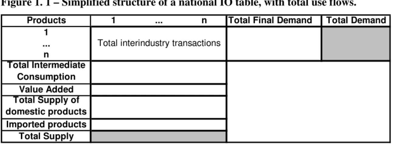
Figure 1. 1 – Simplified structure of a national IO table, with total use flows.

Products 1 ... n Total Final Demand Total Demand

1 ... n Total Intermediate Consumption Value Added Total Supply of domestic products Imported products Total Supply

Total interindustry transactions

Looking across the rows in this table, we can observe how the output of each product is used throughout the several consumers of this economy: the total output of each product i (x_i) is used for intermediate consumption by the various industries j and for the diverse final demand purposes. As mentioned in the Figure’s label, this is a total flow table, meaning that the flows recorded as intermediate and final demand refer not only to domestically produced input, but also to imported input. The columns of Figure 1. 1 provide information on the input composition of the total supply of each product j (xj):

this is comprised by the national production and also by imported products. The value of domestic production consists of intermediate consumption of several industrial inputs i plus value added5. The interindustry transactions table is a nuclear part of this table, in the sense that it provides a detailed portrait of how the different economic activities are interrelated. Since, in this table, intermediate consumption is of the total-flow type, this implies that true technological relationships are being accounted for. In fact, each column of the intermediate consumption table describes the total amount of each input i

4

Intermediate consumption consists in the value of products “which are used or consumed as inputs in the process of production during a specific accounting period.” (Jackson, 2000, p.110)

5

Value added is measured by the payments made for other production factors, like labour and capital (thus including compensation of employees, profits and capital consumption allowances).

consumed in the production of output j, regardless of the geographical origin of that input.

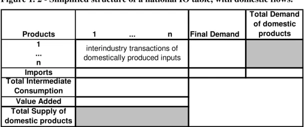
Figure 1. 2 - Simplified structure of a national IO table, with domestic flows.

Products 1 ... n Final Demand

Total Demand of domestic products 1 ... n Imports Total Intermediate Consumption Value Added Total Supply of domestic products interindustry transactions of domestically produced inputs

In alternative, input-output interconnections can be presented considering only domestically produced products in the inputs to be used in intermediate and final consumption. In such case, the table will have a different structure, illustrated in Figure 1. 2 above.

Three major differences exist between this table and the former:

1) The amounts of products used in intermediate consumption by the several industries and by the various final users comprise only domestically produced inputs. In this case, the interindustry transactions table is no longer representative of a technological matrix. It rather represents the intra-national interindustry transactions, which are determined not only by technological factors, but also by trade factors.

2) The row referring to imports has a different arrangement in the table and also a different meaning. Instead of being disaggregated by products and included in the intermediate and final demand flows (as they were in the total-flow table), the imported inputs are now lumped together in a single row, which must be added to the total intermediate consumption of domestic inputs (and to the total final

demand of domestic products), in order to get the total amount of intermediate consumption made by each industry (and the total amount of each component of final demand). Thus, each element of this row gives us the aggregate amount of imports used by each industry and by each kind of final user. Conversely, the row of imported products in the total-flow table depicts the total amount of imports of each product j ( j=1 L, ,n). These are added to domestic production, in order to obtain the value of total supply by product. So, in the total-flow table, the row of imported products depicts imports disaggregated by products, whereas in the domestic-flow table, it represents imports disaggregated by destination industry.

3) As a consequence, the balance between supply and demand in the total-flow table includes imported products, whereas in the domestic-flow table this balance is made considering only domestic production.

The dichotomy between total use and domestic flows will be a recurring issue in the following sections and it will be analysed with further detail in section 1.5.3. In the following nation-level input-output model deduction, we will assume a total-use table as the starting point. The comparison between the total-use model and the model correspondent to Figure 1. 2 is left to section 1.3.1, in which a single-region case is considered. In fact, the structure of single-region models is very similar to the structure of single-nation models, as we will see in section 1.3.1.

The input-output interconnections illustrated in Figure 1. 1 can be translated analytically into accounting identities. On the demand perspective, if we let z_ij denote the intermediate use of product i by industry j and y_i denote the final use of product i, we may write, to each of the n products:

... ... 2 1 i ii in i i i z z z z y x = + + + + + + (1. 1)

m ... ... j 2 1 + + + + + + + = _{j j jj nj j} j z z z z w x (1. 2)

in which w_j stands for value added in the production of j and m_j for total imports of product j. Of course, it is required that, for i= , j xi =xj, i.e., for one specific product,

the total output obtained in the use or demand perspective must equal the total output achieved by the supply perspective.

These two equations can be easily related to the National Accounts identities. Let’s use the following notation for the macroeconomic variables: C represents private consumption; F represents gross capital formation; G stands for government consumption; E and M denote exports and imports, respectively and VA means value added. All these variables represent aggregate values. Let’s consider also the following sums:

∑

∑

Then, if we sum up all the equations (1. 1), we get the total value of all economic activity in this economy (Miller, 1998):

∑

∑

∑

∑

, the previous equation becomes:

E G F C z x n i i n i i =

∑

∑

Similarly, if we sum up all the equations (1. 2), we must achieve the same value. This corresponds to: M VA z x n j j n j j =

∑

∑

∑

∑

are equal, since both represent the sum of all elements of the

intermediate consumption matrix (

∑

∑

∑∑

Since VA represents the sum of the value added generated by all producers in the economy, it corresponds to the economy’s gross domestic product (GDP)6 accounted by a product approach. So, equation (1. 6) is precisely the well known macroeconomic identity between GDP when it is defined by a product approach and the same concept, defined according to the expenditure perspective:

) (E M G F C GDP= + + + − (1. 7)

Let’s refer back to the disaggregate level, embodied in equations (1. 1) and (1. 2). These are merely the mathematical representation of the information displayed in any input-output table, for a certain base-year. In order to introduce the input-input-output model we need to consider the fundamental concept of technical coefficient (Miller, 1998): _ij

j ij a x z = , 6

In National Accounts, the aggregate value added differs from GDP, by the amount of the aggregate taxes (less subsidies) on products; i.e., it is valued at basic prices, while GDP by default, as it is defined on the

which gives us the total amount of product i (domestically produced and imported) used as input in the production of one monetary unit of industry j’s output. Using this definition, equation (1. 1) may be substituted for:

i n in i ii i i i a x a x a x a x y x = 1 1 + 2 2 +...+ +...+ + (1. 8)

Replicating this to each of the n products under consideration and rearranging terms in the equation, we have:

n n nn i ni n n i n in i ii i i n n i i n n i i y x a x a x a x a y x a x a x a x a y x a x a x a x a y x a x a x a x a = − + − − − − − = − − − + − − − = − − − − − + − = − − − − − − ) 1 ( ... ... ... ... ... ) 1 ( ... ... ... ... ... ) 1 ( ... ... ) 1 ( 2 2 1 1 2 2 1 1 2 2 2 2 22 1 21 1 1 1 2 12 1 11 (1. 9)

or, in matrix terms:

                    =                                           − − − − − − − − − − − − − − − − n i n i nn ni n n in ii i i n i n i y y y y x x x x a a a a a a a a a a a a a a a a M M M M M M M M M M M M M M M M 2 1 2 1 2 1 2 1 2 2 22 21 1 1 12 11 ... ... ... ) 1 ( ... ... ... ) 1 ( ... ... ) 1 ( (1. 10)

which may be translated into a compact form:

y A) (I x y x A) (I 1 − − = ⇔ = ⋅ − (1. 11)

In this equation, A is the technical coefficient matrix (total use flows); x is the total output column vector and y is the final use column vector. From equation (1. 11), the popular input-output impact analysis can be carried out straightforwardly. Assuming a small exogenous change in the final use vector (by the amount ∆y), the correspondent change in the output vector (∆x) can be obtained as follows:

y B x y A) (I x 1 ∆ = ∆ ∆ − = ∆ − (1. 12)

There is a proportionality hypothesis embodied in this equation. It is assumed that the change occurred in the output vector is a constant proportion (given by (I−A)−1) of the change in the final demand vector. This fixed proportion implies that the technical coefficients comprised in matrix A do not change with the exogenous impact in final demand, which is a reasonable hypothesis if we consider a small impact ∆y. 1

A) (I− − or B is the so-called Leontief inverse. Each of its elements b_ij traduces the value of output i required directly and indirectly to deliver one additional monetary unit to j’s demand (Miller, 1998)7. In analytical terms,

j i ij y x b ∂ ∂

= . If we sum up each column of this

inverse matrix, we obtain

∑

, which are the output multipliers8. These represent the value of the economy-wide output required directly and indirectly to deliver one additional monetary unit to j’s demand. In other words, they measure the impact over all the economy caused by a change in the final demand for output j.

7

It should be noted that output i may either be domestically produced or imported. Also, the initial impact over product j is not exclusively directed to domestic production, but is indifferent to the geographic origin of the product. Further on this Chapter, we will present alternative multipliers which measure specifically the impact over domestic production.

8

Other types of multipliers can be computed. For example, if we weight the elements of the inverse matrix by appropriate employment coefficients, we can deduce employment multipliers, measuring the impact on

The Leontief inverse can also be approximated through a mathematical series expansion. Given that the technical coefficients matrix verifies the conditions of being “(…) a square matrix A in which all elements are nonnegative and less than one, and in which all column sums are less than one” (Miller, 1998, p. 53), the inverse (I−A)−1 can be expanded using the following power series expression9:

L L_{+ +} + + + + = − −1 2 3 k A A A A I A) (I (1. 13)

This expression highlights the presence of different types of effects (initial, direct and indirect effects)10 caused by an exogenous change in final demand (Miller, 1998). Inserting equation (1. 13) into (1. 12), we get:

(

)

From this equation we can see that, when the vector of final demand changes, this causes an initial effect of the same amount on the output vector, given by the first term: ∆y. To satisfy these new productions, industries will have to buy some new inputs, given by

y

A∆ - these are the direct effects. The remaining terms capture the indirect effects caused by the fact that the production of those new inputs also requires intermediate consumption of additional inputs. Of course, as it happens in any power series expansion, as the exponent increases, the correspondent effect decreases, implying that the latter indirect effects will be necessarily smaller than the former indirect effects and than the direct effects.

9

This results is similar to that of ordinary algebra, according to which a power series of infinite terms like L L_{+ +} + + + + k r r r r 2 3

1 is equal to

(

)

10

Sometimes, initial and direct effects are lumped together and considered both as direct effects. This is why Leontief inverse is also known by the matrix of direct and indirect requirements.

Some hypotheses are implicit in the kind of reasoning exposed above, frequently pointed out as limitations of input-output (mainly when it is used as a forecast model): firstly, the elements of matrix A are assumed to be time-invariant, meaning that the underlying technology is constant – obviously, this is a restrictive assumption in long-run forecast applications of the model, making it more suitable to short-run uses; second, it is assumed that the aij are the same, irrespective of the scale of production (constant returns to scale),

which implies that scale economies are not taken into account; thirdly, the assumption of constant aij also implies that we are dealing with a fixed proportion technology; in fact, if

we consider two inputs, i and k, to produce output j, the proportion in which they are used

is given by , kj ij j kj j ij kj ij a a x a x a z z =

= which is constant, since the technical coefficients are also

constant (Miller e Blair, 1985); finally, the production capacity is supposed to be unlimited: when the final use of some product increases it is supposed that the output of this product and the others will be able to answer the additional direct and indirect requirements, without any capacity restrictions. With the aim of overcoming these shortcomings of the model, several developments have been introduced into the basic formulation: for instance, dynamic models that consider varying technical coefficients and models that include capacity restrictions. Yet, in the present work, the basic formulation will be used, since forecasting impacts is not our primary objective.

1.3.

Regional input-output models.

In spite of having been originally conceived to national-wide applications, input-output model has been applied to sub-national geographic units since the second half of the last century. According to Miller and Blair (1985), there are two specific features associated to the regional dimension which make evident and necessary the distinction between national and regional input-output models. First, the technology of production of each region is specific, and it may be close or, on the contrary, very different from the one

industries, the characteristics of input markets or the education level of the labour force are important factors that may influence the regional technology of production to deviate from the national one. Second, the smaller the economy under study, the more it depends on the exterior world, making more relevant the exported and imported components of demand and supply, respectively. It should be noted that these components correspond not only to international trade, but also to the trade between the region and the rest of the country to which the region belongs.

In this section we aim to review the main contributions in regional input-output modelling. The following models are distinguishable by four main criteria:

- the number of regions taken into account: single-region or many-region models. - the recognition (or not) of interregional linkages;

- the degree of detail implicit in interregional trade flows (which is related to the degree of detail demanded for the input-output data) and

- the kind of hypotheses assumed to estimate trade coefficients.

We will begin by presenting the single-region model (section 1.3.1), which has a similar structure to the nation level input-output model presented in the previous section. Then we proceed to those models that try to capture, not only intra-regional transactions, but also the interconnections between regions. Of these, we begin by reviewing Leontief’s intranational model (section 1.3.2), which consists of a very primary type of regional input-output model, since the only spatial effect it recognizes concerns to the one-way effect of national changes over regional output. As it will be seen, spillover and feedback regional effects are not considered by this model. The remaining models (sections 1.3.3. to 1.3.5) seek to account for inter-spatial effects. Yet, they differ in the degree of detail used in the specification of interregional trade flows. Besides, the two multi-regional models (Chenery-Moses and Riefler-Tiebout) are distinct by the hypotheses they assume to determine trade coefficients. One common feature of the last three regional models is

the fact that trade coefficient stability is assumed. We will give special attention to this aspect on section 1.3.6.

1.3.1 Single-region model.

The aim of single-region input-output models is to evaluate the impact on regional output caused by changes in regional final demand. The starting point for a single-region model is, obviously, a single-region input-output table. Just like it happened in the nation-level table, exposed in the previous section, the single-region input-output table may be presented in two different versions: as a total-use table or as an intra-regional flow table11. The correspondence between the structure of these two regional tables and the national tables presented above is straightforward. If we consider that, in Figure 1. 1, the row of imported products includes also imports from other regions of the same country and the vector of final demand comprises also exports to the rest of the country, then this table represents a single-region input-output table, with total use flows. Correspondingly, if we take similar considerations over the table in Figure 1. 2 (concerning imports and exports) and consider additionally that the intermediate and final use flows include only regionally produced inputs, then Figure 1. 2 is converted into a single-region input-output table, with intra-regional flows. These two types of data arrangement originate two different single-region models: (1) total-use single-region model and (2) intra-regional single-region model.

The development of the total-use single-region model follows closely the development of the nation-level input-output model made in the previous section. Let’s use the superscript r to denote a regional variable; thus, for example x_ir is the amount of output i available in region r (including international and interregional imports), y_ir represents regional final demand for product i (including the one that consists of imported products) and z_ijr denotes the total amount of input i used in the production of output j in region r

(including imported inputs as well). Then, _r j r ij r ij x z

a = is the regional technical coefficient, defined in a similar way as the national one. This indicates the amount of input i necessary to produce one monetary unit of output j in region r. In should be stressed out that all the possible geographic origins of input i are being included in the calculation of this coefficient, meaning that zijr comprises product i produced in region r but also

produced in other regions or even abroad, since it is traded in region r. Using the regional variables instead of the national ones, we can write an equation similar to equation (1. 1):

... ... 2 1 r i r in r ii r i r i r i z z z z y x = + + + + + + (1. 15)

Considering the regional technical coefficient _r

j r ij r ij x z

a = , this equation becomes:

r i r n r in r i r ii r r i r r i r i a x a x a x a x y x = 1 1 + 2 2 +...+ +...+ + (1. 16)

The compact matrix representation correspondent to the previous equation (considering one equation like this to each of the n products) is:

r 1 r r r r r y ) A (I x y x ) A (I − − = ⇔ = ⋅ − (1. 17)

This solution allows us to quantify the impact over the total output available at region r caused by a change in regional final demand. Similarly to what was done at the national level, we may write:

r 1 r r y ) A (I x = − ∆ ∆ − (1. 18)

It should be noted that this impact is not limited to the region itself; instead, some of the impact measured by this equation is felt outside the region, via effect on imported products (included in the values of vector r

over regional production from the total-use model. If we pre-multiply both sides of the previous equation by

(

)

Let’s now consider an intra-regional input-output table (similar to the one in Figure 1. 2) as the starting point to the input-output model development. The major difference relies on the type of coefficient used: instead of the regional technical coefficient, it is used a coefficient that indicates the amount of regionally produced input i necessary to produce one monetary unit of output j in region r. This is called an intra-regional input coefficient, being this label sometimes simplified to regional input coefficient (Miller and Blair, 1985). Let zijrr denote the amount of regionally produced input i used in the production of

output j in region r. Then, the intra-regional input coefficient may be computed as:

r j rr ij rr ij e z

a = , in which erj denotes regional production of product j. Considering

additionally f_ir as the region’s final demand towards product i produced in region r (including regional requirements as well as exports for any other regions, national or foreign), the solution of the single-region input-output model with intra-regional flows follows the same procedures as before. In matrix terms, let’s use the notation:

• rr

A - a matrix composed by intra-regional input coefficients a_ijrr;

• r

e - the vector of output produced in region r; • r

f - the vector of regional final demand towards products produced in region r.