doi: 10.5540/tema.2018.019.02.0305
A Comparison Among Simple Algorithms for Linear Programming
J. SILVA1*, C.T.L.S. GHIDINI2, A.R.L. OLIVEIRA3and M.I.V. FONTOVA4
Received on July 28, 2017 / Accepted on March 10, 2018
ABSTRACT.This paper presents a comparison between a family of simple algorithms for linear program-ming and the optimal pair adjustment algorithm. The optimal pair adjustment algorithm improvements the convergence of von Neumann’s algorithm which is very attractive because of its simplicity. However, it is not practical to solve linear programming problems to optimality, since its convergence is slow. The family of simple algorithms results from the generalization of the optimal pair adjustment algorithm, including a parameter on the number of chosen columns instead of just a pair of them. Such generalization preserves the simple algorithms nice features. Significant improvements over the optimal pair adjustment algorithm were demonstrated through numerical experiments on a set of linear programming problems.
Keywords: Linear programming, von Neumann’s algorithm, Simple algorithms.
1 INTRODUCTION
The von Neumann algorithm was reported by Dantzig in the early 1990s [4, 5], and it was later studied by Epelman and Freund [7], and Beck and Teboulle [1]. Some of the advantages pre-sented by this method are its low computational cost per iteration, which is dominated by the matrix-vector multiplication, in addition to its ability to exploit the data sparsity from the orig-inal problem and the usually fast initial advance. Epelman and Freund [7] refer to this algo-rithm as “elementary”, since each iteration involves only simple computations; therefore, it is unsophisticated, especially when compared with the modern interior point algorithms.
In [11], three algorithms were proposed to overcome some convergence difficulties from von Neumann’s method: the optimal pair adjustment algorithm, the weight reduction algorithm,
*Corresponding author: Jair Silva – E-mail: [email protected]
1Campus Avanc¸ado da Universidade Federal do Paran´a em Jandaia do Sul, Rua Doutor Jo˜ao Maximiano, 426, Vila Oper´aria, 86900-000, Jandaia do Sul, PR, Brazil. E-mail: [email protected]
2Faculdade de Ciˆencias Aplicadas, Universidade de Campinas, Rua Pedro Zaccaria, 1300, 13484-350, Limeira, SP, Brazil. E-mail: [email protected]
3Instituto de Matem´atica, Estat´ıstica e Computac¸˜ao Cient´ıfica, Universidade de Campinas, Rua S´ergio Buarque de Holanda, 651, 13083-859, Campinas, SP, Brazil. E-mail: [email protected]
and projection algorithm. The optimal pair adjustment algorithm (OPAA) provides the best results among them. This algorithm inherits the best properties from von Neumann’s algo-rithm. Although OPAA has a faster convergence when compared to von Neumann’s algorithm, its convergence is also considered slow, making it impractical for solving linear optimization problems.
This work presents a comparison between a family of simple algorithms for linear programming and the optimal pair adjustment algorithm. This family originated from the generalization of the idea presented by Gonc¸alves, Storer and Gondzio in [11] to develop the OPAA. Hence, the optimal adjustment algorithm forpcoordinates was developed. Indeed, for different values ofp, a different algorithm is defined, in whichpis limited by the order of the problem, thus resulting in a family of algorithms. This family of simple algorithms maintains the ability to exploit the sparsity from the original problem and a fast initial convergence. Significant improvements over OPAA are demonstrated through numerical experiments on a set of linear programming problems.
The paper is organized as follows. Section 2 contains a description of von Neumann’s algorithm. Section 3 presents both the weight reduction algorithm and the OPAA. Section 4 discusses the family of simple algorithms, theoretical properties of convergence of the optimal adjustment algorithm for p coordinates, and a sufficient condition for it to present better iterations than the iterations of von Neumann’s algorithm. Section 5 describes the computational experiments comparing the family with the OPAA. The conclusions and perspectives for future work are presented in the last section.
2 THE VON NEUMANN’S ALGORITHM
The von Neumann algorithm for solving linear programming problems was first described by Dantzig in the early 1990s in [4, 5]. Such an algorithm actually solves the equivalent problem described below.
Consider the following set of linear constraints and the the search for a feasible solution for:
Px=0,
etx=1,x≥0, (2.1)
whereP∈ℜm×nand||P
j||=1 for j=1, . . . ,n(the columns have norm one),x∈ℜn,e∈ℜnis the vector with all ones.
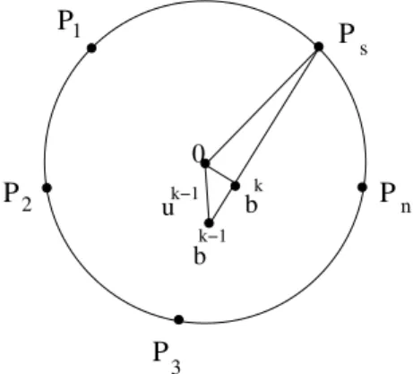
Geometrically, the columns Pj are points on them-dimensional hypersphere with unit radius and center at the origin. Therefore, the above problem assigns non-negative weightsxj to the Pj columns so that its origin is the rescaled gravity center. Note that any linear programming problem can be reduced to problem (2.1) (see [10]).
that forms the largest angle with the residualbk−1. The trianglebk−10bkhas as hypotenuse 0bk−1 and cathetus 0bk, and thus,||bk||<||bk−1||for all iterations.
P
2
P
3
n
P
s
P
1
uk−1
b
k−1
b
k
P
0
Figure 1: Illustration of von Neumann’s algorithm.
The steps of von Neumann’s algorithm are described below:
Algorithm 1:von Neumann’s Algorithm
1 begin
2 Given: x0≥0, withetx0=1.Compute b0=Px0. 3 Fork=1,2,3, ...Do:
4 1)Compute:
5 s=argminj=1,...,n{Ptjbk−1}, 6 vk−1=Pstbk−1.
7 2)If vk−1>0,thenSTOP. The problem (2.1) is infeasible. 8 3)Compute:
9 uk−1=||bk−1||, λ = 1−v
k−1
(uk−1)2−2vk−1+1.
10 4)Update:
11 bk=λbk−1+ (1−λ)Ps, xk=λxk−1+ (1−λ)es, 12 whereesis the standard basis vector with 1 in thes-th coordinate.
13 end
In computational experiments, the stopping criterion was||bk−bk−1||/||bk||<ε, whereε is a specified tolerance, andx0j=1
n,j=1, . . . ,nwas considered.
3 THE WEIGHT REDUCTION AND THE OPTIMAL PAIR ADJUSTMENT ALGORITHMS
In this section, two algorithms developed by Gonc¸alves [11] are described. The algorithms are based on von Neumann’s algorithms and were developed to improve convergence. They are the weight-reduction algorithm and the optimal pair adjustment algorithm.
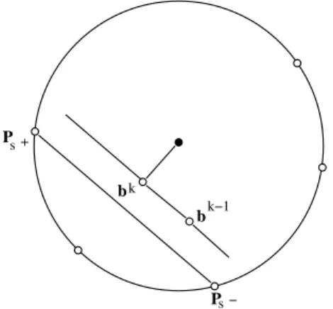
In the weight-reduction algorithm, the residualbk−1is moved closer to the origin 0 by increasing the weightxjof some columnsPjor decreasing the weightxiof other columnsPi. Figure 2 shows the geometric interpretation of the weight-reduction algorithm.
Ps − +
s
bk
P
bk−1
Figure 2: Illustration of the weight-reduction algorithm.
At each iteration, the residualbk−1 moves in the direction P
s+−Ps− where the columns Ps+
andPs− make the largest and smallest angle withbk−1, respectively. The new residualbkis the projection of the origin in that line. Only the weightsx+andx− will be changed. There is no
guarantee that an iteration of this algorithm will improve as much as an iteration of the von Neumann algorithm [11].
However, the OPAA also developed by Gonc¸alves improves the residual at least as much as the von Neumann algorithm [11].
First, the OPAA calculates the columnsPs+ andPs−. Then, the algorithm computes the values xk
s+,x k
s− andλ wherex k
j=λxkj−1for all j6=s+and j6=s−that minimize the distance between bkand the origin, subject to the convexity and the non-negativity constraints. The solution to this optimization problem is easy to find by examining the Karush-Kuhn-Tucker (KKT) conditions (see [11]).
The optimal pair adjustment algorithm is described below.
The OPAA modifies all the weightsxk
Algorithm 2:Optimal Pair Adjustment Algorithm
1 begin
2 Given: x0≥0, with etx0=1. Compute b0=Px0. 3 Fork=1,2,3, ...Do:
4 1)Compute:
5 s+=argminj=1,...,n{Ptjbk−1},
6 s−=argmaxj=1,...,n{Pjtbk−1| xj>0}, 7 vk−1=Pt
s+b k−1.
8 2)If vk−1>0,thenSTOP; the problem (2.1) is infeasible. 9 3)Solve the problem:
10
minimize ||b||2
s.t. λ0(1−xks−+1−xks−−1) +λ1+λ2=1, λi≥0, fori=0,1,2.
(3.1)
11 where,b=λ0(bk−1−xk−1
s+ Ps+−xks−−1Ps−) +λ1Ps++λ2Ps−. 12 4)Update:
13
bk=λ0(bk−1−xks+−1Ps+−xks−−1Ps−) +λ1Ps++λ2Ps−,
xk j=
λ0xkj−1, j=6 s+e j6=s−, λ1, j=s+,
λ2, j=s−. k=k+1.
14 end
4 OPTIMAL ADJUSTMENT ALGORITHM FORPCOORDINATES
This section presents the optimal adjustment algorithm for p coordinates developed by Silva [12]. This algorithm was developed by generalizing the idea presented in the subproblem (10) of the OPAA. Instead of using two columns to formulate the subproblem, any number of columns can be used, thus assigning relevancy to any number of variables. For each value ofp, a different algorithm can be formulated. Thus, a family of algorithms was developed.
Thepvariables can be chosen by a different method according to the problem. A natural choice is to takep/2 columns that make the largest angle with the vectorbkandp/2 columns that make the smallest angle with the vectorbk. Ifpis an odd number, an extra column for the set of vectors is taken, which form the largest angle with the vectorbk, for instance.
The steps of the optimal adjustment algorithm for p coordinates are similar to those for the OPAA. First, thes1ands2columns are identified; the s1 ands2columns form the largest and the smallest angle with the residualbk−1, respectively, wheres
1+s2=pandpis the number of columns to be prioritized. Next, the subproblem is solved, and then, the residual and the current point are updated.
Algorithm 3:Optimal Adjustment Algorithm forpCoordinates
1 begin
2 Given: x0≥0, withetx0=1. Compute b0=Px0. 3 Fork=1,2,3, ...Do:
4 1)Compute: 5
{Pη+
1, . . . ,Pηs+1}forming the largest angle with the vectorb k−1.
{Pη−
1, . . . ,Pηs−2} forming the smallest angle with the vectorb
k−1 such as
xki−1>0,i=η1−, . . . ,ηs−
2,wheres1+s2=p.
vk−1=minimumi=1 ,...,s1{P
t
ηi+b
k−1}.
6 2)If vk−1>0, then STOP; the problem (2.1) is infeasible. 7 3)Solve the problem:
8
minimize 12||Aλ||2 s.t. ctλ =1, λ ≥0,
(4.1)
9 whereA=
h w Pη+
1 . . .Pηs+1Pη1−. . .Pηs−2 i
,w=bk−1− s1
∑
i=1 xηk−+1
i
Pη+
i −
s2
∑
j=1 xk−1
η−j
Pη− j ,
λ =λ0,λη+
1, . . . ,ληs+1,λη1−, . . . ,ληs−2
,c= (c1,1, . . . ,1)and
c1=1− s1
∑
i=1 xk−1
ηi+ −
s2
∑
j=1 xk−1
η−j .
10 4)Update:
bk=Aλ∗,
xk j=
λ0xkj−1, j∈ {/ η1+, . . . ,ηs+1,η −
1, . . . ,ηs−2},
λη+
i , j=η
+
i ,i=1, . . . ,s1, λη−
j , j=η
−
j ,j=1, . . . ,s2. k=k+1.
Subproblem (8) was built in such a way that the residual has the maximum decrease, such that, x0≥0, withetx0=1.
4.1 Relation between von Neumann’s algorithm and the algorithm with ppp === 111 and geometric interpretation
The optimal adjustment algorithms forpcoordinates withp=1 and von Neumann’s algorithm generate the same pointsxkand the same residualbkas shown in Figure 1.
The optimalλ for von Neumann’s algorithm is calculated by the projection of the origin in the segment of line joiningbk−1toPs.
In the algorithm when p=1, the following subproblem is solved.
minimize ||b||2
s.t. λ0(1−xks−1) +λ1=1, λi≥0, fori=0,1.
(4.2)
where,b=λ0(bk−1−xsk−1Ps) +λ1Ps.
The subproblem can be rewritten (4.2) as follows:
λ0(1−xsk−1) +λ1=1⇔λ1=1−λ0(1−xks−1)≥0
b =λ0(bk−1−xsk−1Ps) +λ1Ps
=λ0(bk−1−xks−1Ps) + (1−λ0(1−xks−1))Ps
=λ0bk−1+ (1−λ0)Ps.
(4.3)
Thus, the problem (4.2) will be:
minimize ||b||2
s.t. λ∈h0, 1
1−xks−1 i
(4.4)
where,b=λbk−1+ (1−λ)Ps.
If the term 1
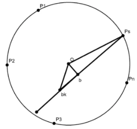
1−xks−1 is larger than 1, then there will be an increase in the number of possible solutions in comparison with von Neumann’s algorithm. Although, the geometric interpretation of the algorithm with p=1 presented in Figure 3 show that the optimalλ is the same for both algorithms.
In Step 4 of von Neumann’s algorithm,xkis updated by
xk j=
(
Figure 3: Illustration of the algorithm withp=1.
In Step 4 of the algorithm withp=1,xkis updated by
xkj=
(
λxkj−1, j6=s 1−λ(1−xsk−1), j=s.
Therefore, the algorithm withp=1 and von Neumann’s algorithm generate the same pointsxk and the same residualbk.
Forp=2, the subproblem (8) is reduced to the following form:
minimize ||b||2
s.t. λ0(1−xks−+1−xks−−1) +λ1+λ2=1, λi≥0, fori=0,1,2.
(4.5)
where,b=λ0(bk−1−xks+−1Ps+−xks−−1Ps−) +λ1Ps++λ2Ps−.
The termbcan be rewritten as:
b= λ0(bk−1−xks+−1Ps+−xks−−1Ps−) +λ1Ps++λ2Ps−
= λ0bk−1+ (λ1−λ0xks+−1)Ps++ (λ2−λ0xks−−1)Ps−
Thus,b(λ0,λ1,λ2)is a linear transformation. When the vectors{(bk−1−xks+−1Ps+−xsk−−1Ps−),Ps+
ePs−}are linearly independent, such linear transformation is injective. It transforms the triangle generated byλ0(1−xks+−1−xks−−1) +λ1+λ2=1 and its interior into the triangle whose vertices arePs+,Ps−andPv=(1 1
−xk−1 s+−x
k−1 s− )
(bk−1−xks+−1Ps+−xks−−1Ps−), and its interior.
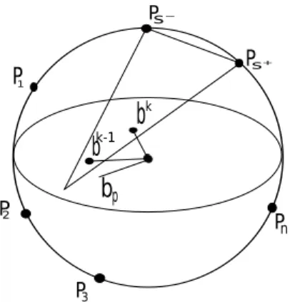
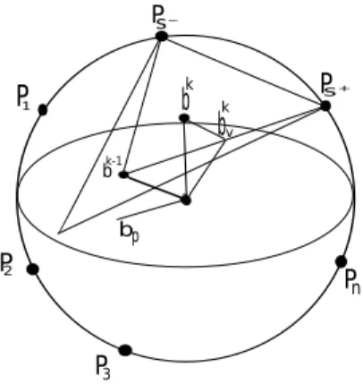
Therefore, the optimal residualbkis the projection of the origin on this triangle. The geometric interpretation of the algorithm withp=2 is given in Figure 4.
P
P
s s
b
kb
k-1b
P
1 P P P 2 3 n pFigure 4: Illustration of the algorithm withp=2.
b= λ0 bk−1− s1
∑
i=1 xk−1
ηi+Pηi+−
s2
∑
j=1 xk−1
η−j Pη−j
!
+
s1
∑
i=1 λη+
i Pηi++ s2
∑
j=1 λη−
j Pη−j
= λ0bk−1+ s1
∑
i=1
(λη+
i −λ0x k−1
ηi+)Pηi++
s2
∑
j=1
(λη− j −λ0x
k−1
η−j )Pη−j
withλ0+ s1
∑
i=1
(λη+
i −λ0x k−1
ηi+)+
s2
∑
j=1
(λη− j −λ0x
k−1
η−j ) =1,thenbis also an affine combination. Then,
the optimal residualbkis the projection of the origin on the affine space region with vertices in thepcolumns and in vectorPv,and
Pv=
1
1−
s1
∑
i=1 xk−1
ηi+ − s2
∑
j=1 xk−1
η−j
bk−1− s1
∑
i=1 xk−1
ηi+Pηi+−
s2
∑
j=1 xk−1
η−j Pη−j
! .
4.2 Subproblem Solution Using Interior Point Methods
In [11], Gonc¸alves solved the subproblem (10) by checking all feasible solutions that satisfies the KKT condition of this subproblem and there are 23−1 possible solutions, see [11]. For the optimal adjustment algorithm forpCoordinates, the possible solutions of the subproblem (8) are 2p−1 [9]. The strategy used by Gonc¸alves in [11] is inefficient even for small values ofp; the number of cases will increase exponentially. The subproblem (8) can be solved by interior point methods.
Consider the subproblem (8). The KKT equations from the problem (8) are given by:
AtAλ+cτ−µ=0, µtλ=0, ctλ−1=0,
−λ≤0,
whereτis a vector of free variables and 0≤µ. The vectorsτandµare the Lagrange multipliers for equality and inequality constraints, respectively, andAtAis a(p+1)×(p+1)matrix.
The path-following interior point method is used to solve the problem (4.6). At each iteration of the interior point method, the linear system of Equation (4.7) is solved to compute the search directions(dλ,dτ,dµ):
AtA c −Id
U 0 Λ
ct 0 0
dλ dτ dµ
=
r1 r2 r3
(4.7)
whereU=diag(µ),Λ=diag(λ),r1=µ−cτ−AtAλ,r2=−τtλ,andr3=1−ctλ.
The directionsdλ,dτanddµare given by:
dµ=Λ−1r
2−Λ−1U dλ, dλ = (AtA+Λ−1U)−1r
4−(AtA+Λ−1U)−1cdτ, ct(AtA+Λ−1U)−1cdτ=ct(AtA+Λ−1U)−1r
4−r3,
wherer4=r1+Λ−1r2.
Consider l1= (AtA+Λ−1U)−1c and l2= (AtA+Λ−1U)−1r4; then, the solution of the lin-ear systems(AtA+Λ−1U)l
1=cand(AtA+Λ−1U)l2=r4 will be necessary to compute the directions.
The matrixAtA+Λ−1Uis a symmetric(p+1)×(p+1)positive definite. Both systems can be solved with the same Cholesky factorization.
4.3 Theoretical Properties of the Family of Algorithms
The theorem 3.1 in [11] ensures that the OPAA converges, in the worst case, with the same rate of convergence as von Neumann’s algorithm. This result can be extended for the optimal adjustment algorithm forpcoordinates, and an increase in the value ofpleads to a more efficient algorithm with improved performance. This is shown in Theorem 4.1. Only the second part will be proved.
Teorema 4.1.The residual||bk||after an iteration of the optimal adjustment algorithm for p coor-dinates is, in the worst case, equal to the residual after an iteration of von Neumann’s algorithm. Furthermore, suppose that||bkp
1||is the residual after an iteration of the optimal adjustment
al-gorithm for p1 coordinates,||bkp2||is the residual after an iteration of the optimal adjustment
algorithm for p2coordinates, and p1≤p2≤n, then||bkp1|| ≤ ||b
k
p2||where n is the number of
columns P.
Proof. Let k ≥1 and bk−1 be the residual at the beginning of the iteration k. Further,
{Pη+
1 , . . . ,Pη+s1}and{Pη1−, . . . ,Pηs−2}are sets of vectors forming the largest and the smallest an-gles with the vectorbk−1, respectively, for the algorithm prioritizing the p
s1+s2= p2; and {Pη+
1 , . . . ,Pηs+3} and {Pη1−, . . . ,Pηs−4} are sets of vectors forming the largest and the smallest angles with the vectorbk−1, respectively, for the algorithm prioritizing the p1 coordinates, wheres3+s4=p1.
After thek-th iteration in the optimal adjustment for the p2coordinates, the residualbkp2 will be
bkp
2=λ1 b
k−1− s1
∑
i=1 xk−1
ηi+
Pη+
i − s2
∑
j=1 xk−1
η−j
Pη− j ! + s1
∑
i=1 λη+i Pηi++ s2
∑
j=1 λη−
j Pη−j ,
where (λ1,λη+
1, . . . ,ληs+1,λη1−, . . . ,ληs−2) is the optimal solution of the subproblem (8) prioritizingp2coordinates.
The optimal solution of the subproblem (8) prioritizingp1coordinates
(eλ1,eλη+
1, . . . ,
e λη+
s3,eλη1−, . . . ,
eλη− s4),
is also a feasible solution for the subproblem (8) whenp2coordinates are prioritized.
Therefore,
eλ1 b
k−1− s3
∑
i=1 xk−1
ηi+Pηi+−
s4
∑
j=1 xk−1
η−j Pη−j
! + s3
∑
i=1 e λη+i Pηi++ s4
∑
j=1 e λη−
j Pη−j
=
=bkp
1
≥bkp
2
,
where bkp
1is the residual after an iteration of the optimal adjustment algorithm for the p1
coor-dinates. Consequently, the reduction of the residual after an iteration of the optimal adjustment algorithm for thep2coordinates is, in the worst case, equal to the reduction of the residual after an iteration of the optimal adjustment algorithm for thep1coordinates.
This theorem does not ensure that one iteration of family of algorithms is better than one iteration of von Neumann’s algorithm. In the next section, we give the sufficient conditions for that to happen.
4.4 Sufficient Conditions for||||||bbbk||||||<<<||||||bbbkv||||||
Letbk be the residual of the algorithm withp=2 in the iterationk, and letPs+ andPs−be the columns forming the largest and smallest angles with the vectorbk−1. If the projection of the origin is in the interior of the trianglebkP
s+Ps− and coincides with the projection of the origin in the plane determined bybk−1,Ps+andPs−,then||bk||<||bkv||,wherebkvis the residual of von
Neumann’s algorithm in the iterationk. In fact, we can see this clearly in Figure 5, noting that the triangle 0bkbk
vhas the 0b k
vhypotenuse and side 0b k
.
P
P
s s
b
kb k-1 b
P
1P
P
P 2
3
n
b
vk
p
Figure 5: Illustration of the Sufficient Condition.
5 COMPUTATIONAL EXPERIMENTS
The algorithm with p=2 is the same of the optimal pair adjustment algorithm. In particular, for the algorithm with p = 2, we could use the same strategy and compute all possible solutions of the subproblem, since there are only 23−1 possible solutions. However, this strategy becomes impractical for larger values of p,so, the strategy is to solve the subproblem by interior point methods for all differents value of p.
We make two experiments. In the first one, the performance of the family of algorithms for moderate values ofpis compared with OPAA, whenp=2. The choice for moderatepvalues comes from the fact that for larger p values, the cost of solution of the subproblem in each iteration becomes noticeable.
The second experiment explores the fact that the optimal adjustment algorithm forpcoordinates allows a dynamic choice ofpconsidering the size of linear problem to be solved. This approach was proposed in [8], the developed heuristic was based on numerical experiments and its given by
0 < (m + n) ≤ 10000 → p = 4;
10000 < (m + n) ≤ 20000 → p = 8;
20000 < (m + n) ≤ 400000 → p = 20;
400000 < (m + n) ≤ 600000 → p = 40;
600000 < (m + n) ≤ → p = 80
wheremis the number of rows andnis the number of columns for the constraint matrixAof the linear problem.
For the all experiments, a collection of 151 linear programming problems is used. The problems are divided into 95 Netlib problems [3], 16 Kennington problems [2], and 40 other problems supplied by Gonc¸alves [11]. These experiments were performed on an Intel Core 2 Quad Q9550 2.83 GHz and 4GB of RAM machine in a Linux using the gcc compiler.
5.1 Implementation Details
The family of algorithms is implemented in C using the format of the problem given in [10] Subsection 2.5.1. The matrix P is not built explicitly. More precisely, it is divided into two blocks. Only one of these blocks is considered in Step 1, at each iteration, to find s1 ands2 columns, which form the largest and smallest angles with residualbk, respectively.
To solve the subproblem, the classical path-following interior point method was implemented in C. The perturbation in the complementarity is(p+1)µtλ2.
The initial point was the point with all coordinates equal to one. The tolerance is 10−12; since the linear equationetx=1 of the problem (2.1) makes each componentxjsmall, if a solution with a good precision is not computed, the method may not work properly.
5.2 Experiment Design
The first experiment was performed following the steps presented by Gonc¸alves, Storer and Gondzio in [11]:
1. Initially, von Neumann’s algorithm is run on all problems;
2. Next, when the relative difference between||bk−1||and||bk||was less than 0.5%, the time t1(CPU seconds) and number of iterations (up tot1) are recorded.
3. Additionally, the timest2,t3,t4, andt5 (CPU seconds), which correspond respectively to 3, 5, 10 and 20 times the number of iterations int1 are also recorded.
4. Next, the optimal adjustment algorithm for pcoordinates, where p=2, p=4, p=10, p=20,p=40 andp=100 is ran on the test problems.
5. Finally, for thetitimes,i=1, . . . ,5, the residual||bk||is recorded.
In the second experiment, both approaches use the termination criteria described in [8]. This is, the experiment stops when the algorithm exceeds its allotted maximum number of iterations (100) or when the relative error of the residual norm is smaller than a tolerance 10−4. The most successful approach is the one with the smaller residual||bk||.
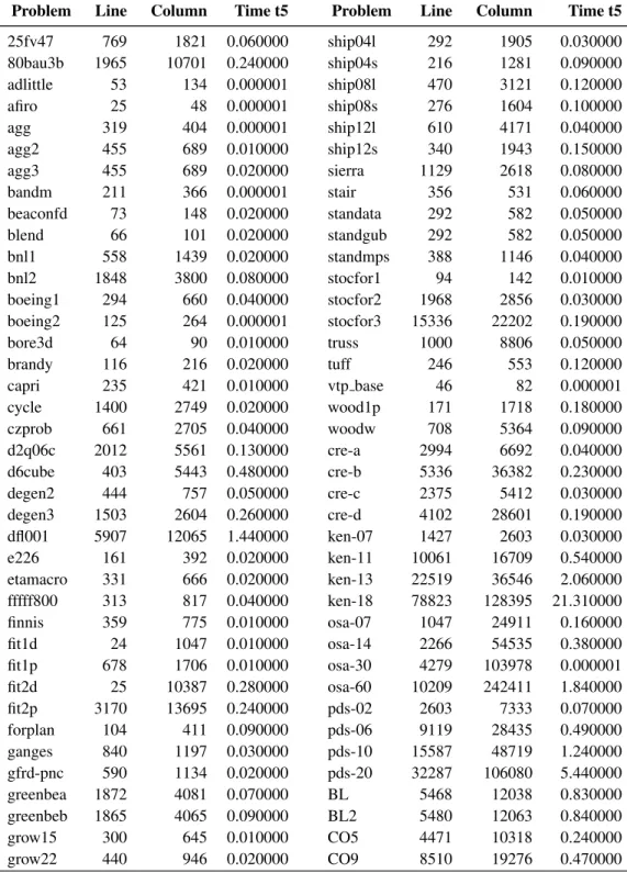
Table 1: Problems test and time t5
Problem Line Column Time t5 Problem Line Column Time t5
25fv47 769 1821 0.060000 ship04l 292 1905 0.030000
80bau3b 1965 10701 0.240000 ship04s 216 1281 0.090000
adlittle 53 134 0.000001 ship08l 470 3121 0.120000
afiro 25 48 0.000001 ship08s 276 1604 0.100000
agg 319 404 0.000001 ship12l 610 4171 0.040000
agg2 455 689 0.010000 ship12s 340 1943 0.150000
agg3 455 689 0.020000 sierra 1129 2618 0.080000
bandm 211 366 0.000001 stair 356 531 0.060000
beaconfd 73 148 0.020000 standata 292 582 0.050000
blend 66 101 0.020000 standgub 292 582 0.050000
bnl1 558 1439 0.020000 standmps 388 1146 0.040000
bnl2 1848 3800 0.080000 stocfor1 94 142 0.010000
boeing1 294 660 0.040000 stocfor2 1968 2856 0.030000
boeing2 125 264 0.000001 stocfor3 15336 22202 0.190000
bore3d 64 90 0.010000 truss 1000 8806 0.050000
brandy 116 216 0.020000 tuff 246 553 0.120000
capri 235 421 0.010000 vtp base 46 82 0.000001
cycle 1400 2749 0.020000 wood1p 171 1718 0.180000
czprob 661 2705 0.040000 woodw 708 5364 0.090000
d2q06c 2012 5561 0.130000 cre-a 2994 6692 0.040000
d6cube 403 5443 0.480000 cre-b 5336 36382 0.230000
degen2 444 757 0.050000 cre-c 2375 5412 0.030000
degen3 1503 2604 0.260000 cre-d 4102 28601 0.190000
dfl001 5907 12065 1.440000 ken-07 1427 2603 0.030000
e226 161 392 0.020000 ken-11 10061 16709 0.540000
etamacro 331 666 0.020000 ken-13 22519 36546 2.060000
fffff800 313 817 0.040000 ken-18 78823 128395 21.310000
finnis 359 775 0.010000 osa-07 1047 24911 0.160000
fit1d 24 1047 0.010000 osa-14 2266 54535 0.380000
fit1p 678 1706 0.010000 osa-30 4279 103978 0.000001
fit2d 25 10387 0.280000 osa-60 10209 242411 1.840000
fit2p 3170 13695 0.240000 pds-02 2603 7333 0.070000
forplan 104 411 0.090000 pds-06 9119 28435 0.490000
ganges 840 1197 0.030000 pds-10 15587 48719 1.240000
gfrd-pnc 590 1134 0.020000 pds-20 32287 106080 5.440000
greenbea 1872 4081 0.070000 BL 5468 12038 0.830000
greenbeb 1865 4065 0.090000 BL2 5480 12063 0.840000
grow15 300 645 0.010000 CO5 4471 10318 0.240000
Table 1 (Continued from previous page)
Problem Line Column Time t5 Problem Line Column Time t5
grow7 140 301 0.000001 CQ9 7073 17806 0.300000
israel 166 307 0.010000 GE 8361 14096 0.200000
kb2 43 68 0.000001 NL 6478 14393 0.560000
lotfi 117 329 0.000001 a1 42 73 0.000001
maros 626 1365 0.030000 fort45 1037 1467 0.060000
maros-r7 2152 6578 0.090000 fort46 1037 1467 0.060000
modszk1 658 1405 0.010000 fort47 1037 1467 0.050000
nesm 646 2850 0.080000 fort48 1037 1467 0.060000
perold 580 1412 0.020000 scagr25 344 543 0.020000
pilot 1350 4506 0.090000 fort49 1037 1467 0.050000
pilot4 389 1069 0.030000 fort51 1042 1473 0.060000
pilot87 1968 6367 0.220000 fort52 1041 1471 0.060000
pilot ja 795 1834 0.040000 fort53 1041 1471 0.050000
pilot we 691 2621 0.050000 fort54 1041 1471 0.050000
pilotnov 830 2089 0.050000 fort55 1041 1471 0.060000
recipe 61 120 0.000001 fort56 1041 1471 0.040000
sc105 104 162 0.000001 fort57 1041 1471 0.060000
sc205 203 315 0.000001 fort58 1041 1471 0.050000
sc50a 49 77 0.000001 fort59 1041 1471 0.050000
sc50b 48 76 0.000001 fort60 1041 1471 0.060000
scagr25 344 543 0.010000 fort61 1041 1471 0.050000
scagr7 92 147 0.000001 x1 983 1413 0.050000
scfxm1 268 526 0.020000 x2 983 1413 0.050000
scfxm2 536 1052 0.030000 pata01 122 1241 0.010000
scfxm3 804 1578 0.040000 pata02 122 1241 0.020000
scorpion 180 239 0.060000 patb01 57 143 0.000001
scrs8 418 1183 0.080000 patb02 57 143 0.000001
scsd1 77 760 0.260000 vschna02 122 1363 0.010000
scsd6 148 1350 0.430000 vschnb01 57 144 0.000001
scsd8 397 2750 0.070000 vschnb02 58 202 0.000001
sctap1 269 608 0.010000 willett 184 588 0.030000
sctap2 977 2303 0.010000 ex01 234 1555 0.070000
sctap3 1346 3113 0.020000 ex02 226 1547 0.070000
seba 2 9 0.130000 ex05 831 7747 0.090000
share1b 107 243 0.040000 ex06 824 7778 0.090000
share2b 92 158 0.010000 ex09 1821 18184 0.340000
5.3 Computational Results
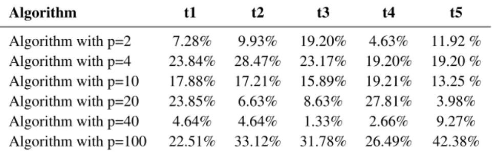
Table 2 shows the relative gain by each algorithm in all problems considering the five different times, i.e., the percentage of problems where the algorithm obtained the lowest value for the residual||bk||, in the timest1 up tot5.
Table 2: Percentage of the relative gain by the algorithms on the problems in five different times
Algorithm t1 t2 t3 t4 t5
Algorithm with p=2 7.28% 9.93% 19.20% 4.63% 11.92 %
Algorithm with p=4 23.84% 28.47% 23.17% 19.20% 19.20 %
Algorithm with p=10 17.88% 17.21% 15.89% 19.21% 13.25 %
Algorithm with p=20 23.85% 6.63% 8.63% 27.81% 3.98%
Algorithm with p=40 4.64% 4.64% 1.33% 2.66% 9.27%
Algorithm with p=100 22.51% 33.12% 31.78% 26.49% 42.38%
According with Table 2, for the optimal adjustment algorithm forp=100 andp=4 coordinates, more problems obtain the lowest value of the residual in comparison with the OPAA (p=2) on the five times. And for p=4, the performance was worse. Especially, the optimal adjustment algorithm forp=100 coordinates had better performance.
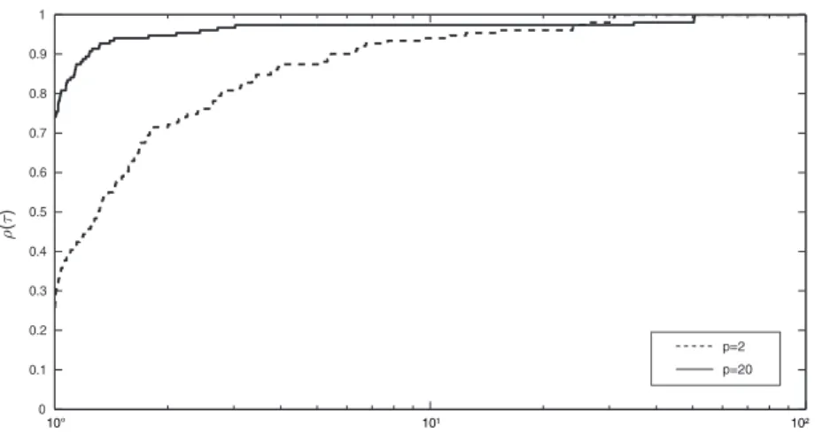
The performances of the algorithms using performance profile [6] was also analyzed. The dis-tance of the residual||bk||to the origin was used to measure the performance. In these graphs, ρ(1)represents the algorithm’s total gain. The best performance algorithms are the ones above the others in graphics.
In Figure 6, the performance profile of the six algorithms with timet5 are compared. This figure shows that the optimal adjustment algorithm forpcoordinates is more efficient than the OPAA (p=2) forp=100, p=10 andp=4. However the algorithm loses in performance forp=20 and p=40. Table 2 shows the performance of the algorithms in the t5 column. In terms of robustness, for all values ofpthe behaviour is the same.
10° 10¹ 10² 0
0.1 0.2 0.3 0.4 0.5 0.6 0.7 0.8 0.9 1
(
)
p=2
p=4
p=10
p=20
p=40
p=100
Figure 6: Performance profile of six algorithms in t5 time.
10¹ 10²
0.1 0.2 0.3 0.4 0.5 0.6 0.7 0.8 0.9 1
p=2
p=100
(
)
Figure 7: Performance profile of the algorithms withp=2 andp=100 in timet5.
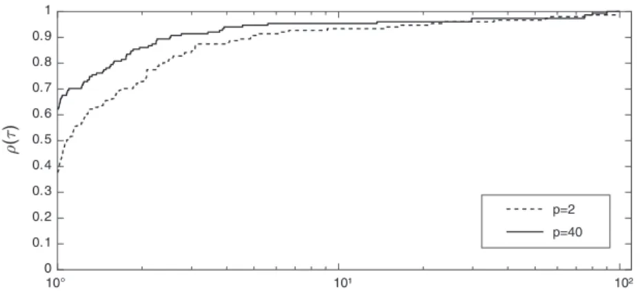
10° 10¹ 10²
0 0.1 0.2 0.3 0.4 0.5 0.6 0.7 0.8 0.9 1
p=2
p=40
(
)
10° 10¹ 10² 0
0.1 0.2 0.3 0.4 0.5 0.6 0.7 0.8 0.9 1
(
)
p=2 p=20
Figure 9: Performance profile of the algorithms withp=2 andp=20 in timet5.
10° 10¹ 10²
0 0.1 0.2 0.3 0.4 0.5 0.6 0.7 0.8 0.9 1
p=2 p=10
(
)
Figure 10: Performance profile of the algorithms withp=2 andp=10 in timet5.
10° 10¹ 10²
0 0.1 0.2 0.3 0.4 0.5 0.6 0.7 0.8 0.9 1
p=2 p=4
(
)
Thus, the performance profiles show that the family of algorithms has good performance for moderatepvalues.
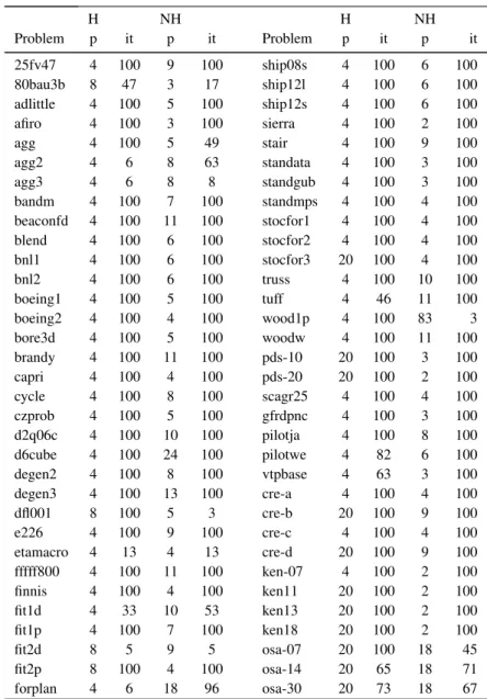
The results obtained in the second experiment are presented in Table 3. The best-performing approach is given by the heuristic p=nz(A)√
mn. It achieves a smaller number of iterations in 52% of the 151 problems tested, a lager number of iterations in 35% of the problems and the same number of iterations in 13% of them. In the Table 3 we present the value ofpand the number of iterations (it) for the approach in [8] (H) and the new heuristic (NH).
Table 3: Heuristic:H×NH
H NH H NH
Problem p it p it Problem p it p it
25fv47 4 100 9 100 ship08s 4 100 6 100
80bau3b 8 47 3 17 ship12l 4 100 6 100
adlittle 4 100 5 100 ship12s 4 100 6 100
afiro 4 100 3 100 sierra 4 100 2 100
agg 4 100 5 49 stair 4 100 9 100
agg2 4 6 8 63 standata 4 100 3 100
agg3 4 6 8 8 standgub 4 100 3 100
bandm 4 100 7 100 standmps 4 100 4 100
beaconfd 4 100 11 100 stocfor1 4 100 4 100
blend 4 100 6 100 stocfor2 4 100 4 100
bnl1 4 100 6 100 stocfor3 20 100 4 100
bnl2 4 100 6 100 truss 4 100 10 100
boeing1 4 100 5 100 tuff 4 46 11 100
boeing2 4 100 4 100 wood1p 4 100 83 3
bore3d 4 100 5 100 woodw 4 100 11 100
brandy 4 100 11 100 pds-10 20 100 3 100
capri 4 100 4 100 pds-20 20 100 2 100
cycle 4 100 8 100 scagr25 4 100 4 100
czprob 4 100 5 100 gfrdpnc 4 100 3 100
d2q06c 4 100 10 100 pilotja 4 100 8 100
d6cube 4 100 24 100 pilotwe 4 82 6 100
degen2 4 100 8 100 vtpbase 4 63 3 100
degen3 4 100 13 100 cre-a 4 100 4 100
dfl001 8 100 5 3 cre-b 20 100 9 100
e226 4 100 9 100 cre-c 4 100 4 100
etamacro 4 13 4 13 cre-d 20 100 9 100
fffff800 4 100 11 100 ken-07 4 100 2 100
finnis 4 100 4 100 ken11 20 100 2 100
fit1d 4 33 10 53 ken13 20 100 2 100
fit1p 4 100 7 100 ken18 20 100 2 100
fit2d 8 5 9 5 osa-07 20 100 18 45
fit2p 8 100 4 100 osa-14 20 65 18 71
Table 3 (Continued from previous page)
H NH H NH
Problem p it p it Problem p it p it
ganges 4 2 4 2 osa-60 20 100 2 9
greenbea 4 54 8 40 pds-02 4 100 3 100
greenbeb 4 100 8 68 pds-06 20 100 3 100
grow15 4 100 6 100 BL 8 100 4 100
grow22 4 100 6 100 BL2 8 100 4 100
grow7 4 100 6 100 CO5 8 100 7 100
israel 4 100 11 100 CO9 20 100 7 100
kb2 4 100 5 100 CQ9 20 100 7 100
lotfi 4 55 5 100 GE 20 6 4 6
maros 4 6 7 72 NL 20 100 4 100
maros-r7 4 28 26 100 a1 4 100 3 100
modszk1 4 25 3 34 fort45 4 62 3 84
nesm 4 100 5 100 fort46 4 100 3 100
perold 4 100 6 100 fort47 4 83 3 100
pilot 4 100 12 54 fort48 4 92 3 100
pilot4 4 100 8 100 fort49 4 34 3 54
pilot87 4 100 14 100 fort51 4 42 4 42
pilotnov 4 100 8 52 fort52 4 100 3 100
recipe 4 100 4 100 fort53 4 100 3 100
sc105 4 100 3 100 fort54 4 36 3 100
sc205 4 100 3 100 fort55 4 34 3 100
sc50a 4 100 3 100 fort56 4 100 3 100
sc50b 4 100 3 100 fort57 4 100 3 100
scagr25 4 100 4 100 fort58 4 100 3 100
scagr7 4 100 3 100 fort59 4 100 3 100
scfxm1 4 100 6 100 fort60 4 100 3 100
scfxm2 4 100 6 100 fort61 4 100 3 100
scfxm3 4 100 6 100 x1 4 4 3 6
scorpion 4 100 4 100 x2 4 100 3 76
scrs8 4 100 5 100 pata01 4 100 7 100
scsd1 4 100 10 100 pata02 4 100 7 100
scsd6 4 100 10 100 patb01 4 100 4 100
scsd8 4 100 9 100 patb02 4 100 4 100
sctap1 4 100 5 100 vschna02 4 100 7 100
sctap2 4 100 5 100 vschnb01 4 100 4 100
sctap3 4 100 5 100 vschnb02 4 100 4 100
seba 4 100 4 100 willett 4 100 8 100
share1b 4 88 7 100 ex01 4 100 5 100
share2b 4 100 7 100 ex02 4 100 5 100
shell 4 68 3 100 ex05 4 100 5 100
ship04l 4 100 6 100 ex06 4 100 5 100
ship04s 4 100 6 100 ex09 20 100 5 100
6 CONCLUSIONS
The family of simple algorithms arose from the generalization of the OPAA. The major advantage of this family of algorithms is its simplicity and fast initial convergence. This paper presents a comparison between a family of simple algorithms for linear programming and the OPAA. Besides, it is proved that the algorithm with p=1 is equivalent to von Neumann’s algorithm. Finally, sufficient conditions show that the family of algorithms has better performance than von Neumann’s algorithm.
The first experiment is performed in a similar framework as reported by in Gonc¸alves, Storer and Gondzio in [11] and the second experiment is performed in a similar framework as reported in [9]. In the first experiment the computational results show the superiority of the family of algorithms for moderate pvalues, in comparison with OPAA. Performance profile graphs indicate that the family of algorithms has significantly more efficiency and robustness. In the second experiment the new heuristicp=nz(A)√mn achieves better results than the approach given in [9].
Despite the improvements with respect to OPAA, the family of algorithms is not practical for solving linear programming problems up to a solution. However, it can be useful in some instances, such as, improving the starting point for interior point methods as in [8], or to work in combination with interior point methods using its initial fast convergence rate as reported in [9]. Nevertheless, future researches are needed to measure the impact that the family of algorithms can have in this direction.
ACKNOWLEDGEMENT
This work was partially funded by the Foundation for the Support of Research of the State of S˜ao Paulo (FAPESP) and Brazilian Council for the Development of Science and Technology (CNPq).
The authors are grateful to the referees for their valuable suggestions which improved this article.
RESUMO. Este artigo apresenta uma comparac¸˜ao entre uma fam´ılia de algoritmos sim-ples para programac¸˜ao linear e o algoritmo de ajustamento pelo par ´otimo. O algoritmo de ajustamento pelo par ´otimo foi desenvolvido para melhorar a convergˆencia do algoritmo de von Neumann que ´e um algoritmo muito interressante por causa de sua simplicidade. Por´em n˜ao ´e muito pr´atico resolver problemas de programac¸˜ao linear at´e a otimalidade com ele, visto que sua convergˆencia ainda ´e muito lenta. A fam´ılia de algoritmos simples surgiu da generalizac¸˜ao do algoritmo de ajustamento pelo para ´otimo, incluindo um parˆametro sobre o n´umero de colunas escolhidas, em vez de manter fixa duas. Esta generalizac¸˜ao preserva a simplicidade dos algoritmos e suas boas qualidades. Apresentamos experimentos num´ericos sobre um conjunto de problemas de programac¸˜ao linear que mostram melhorias significativas em relac¸˜ao ao algoritmo de ajustamento pelo par ´otimo.
REFERENCES
[1] A. Beck & M. Teboulle. A Conditional Gradient Method with Linear Rate of Convergence for Solving
Convex Linear Systems.Mathematical Methods of Operations Research, (2004).
[2] W. Carolan, J. Hill, J. Kennington, S. Niemi & S. Wichmann. An empirical evaluation of the KORBX algorithms for military airlift applications.Oper. Res,38(1990), 240–248.
[3] N. collection LP test sets. NETLIB LP repository.Online at http://www.netlib.org/lp/data.
[4] G.B. Dantzig. Converting a converging algorithm into a polynomially bounded algorithm. Technical report, Stanford University (1991).
[5] G.B. Dantzig. Anε-precise feasible solution to a linear program with a convexity constraint in ε12
iterations independent of problem size. Technical report, Stanford University (1992).
[6] E. Dolan & J. More. Benchmarking optimization software with performance profiles.Math. Program,
(2002), 91:201–213.
[7] M. Epelman & R.M. Freund. Condition number complexity of an elementary algorithm for computing
a reliable solution of a conic linear system.Mathematical Programing,88(2000), 451–485.
[8] C.T.L.S. Ghidini, A.R.L. Oliveira & J. Silva. Optimal Adjustment Algorithm for p Coordinates and
the Starting Point in Interior Point Methods.American Journal of Operations Research, (2011).
[9] C.T.L.S. Ghidini, A.R.L. Oliveira, J. Silva & M. Velazco. Combining a Hybrid Preconditioner and
a Optimal Adjustment Algorithm to Accelerate the Convergence of Interior Point Methods.Linear
Algebra and its Applications,436(2012), 1–18.
[10] J.P.M. Gonc¸alves. “A Family of Linear Programming Algorithms Based on the Von Neumann Algorithm”. Ph.D. thesis, Lehigh University, Bethlehem (2004).
[11] J.P.M. Gonc¸alves, R.H. Storer & J. Gondzio. A Family of Linear Programming Algorithms Based on
an Algorithm by von Neumann.Optimization Methods and Software, (2009).